Statistics of cycles in large networks

Abstract

We present a Markov Chain Monte Carlo method for sampling cycle length in large graphs. Cycles are treated as microstates of a system with many degrees of freedom. Cycle length corresponds to energy such that the length histogram is obtained as the density of states from Metropolis sampling. In many growing networks, mean cycle length increases algebraically with system size. The cycle exponent $\alpha$ is characteristic of the local growth rules and not determined by the degree exponent $\gamma$. For example, $\alpha=0.76(4)$ for the Internet at the Autonomous Systems level.

Physics research into graphs and networks has begun to provide a common framework for the analysis of complex systems in diverse areas including the Internet, biochemistry of living cells, ecosystems, social communities AlbertReview ; DorogovtsevReview ; BornholdtBook . The graph representation of these systems as discrete units coupled by links (nodes and edges) exhibits a large set of scaling phenomena including fractal dimension Song05 and hierarchy of modules Ravasz03 .

A fundamental observation is the scale-free nature of many networks Barabasi99 . The fraction of nodes with a given number of connections, called degree $k$, decays as a power law, $P(k)\sim k^{-\gamma}$ for large $k$. For typical exponents $\gamma<3$, the highly inhomogeneous density of connections can give rise to efficient information transfer Pastor01a and enhanced failure tolerance Albert00 .

Beside the degree distribution and node-node distances, the presence of cycles is a relevant property of networks. A cycle is a closed, not self-intersecting path. Initially, mainly cycles of the minimal length $h=3$ were considered since high abundance of triangles is taken as a sign of a clustered structure Watts98 . Longer cycles gained attention recently. Approximations for the system size scaling of the number $c(h)$ of cycles of length $h$ have been derived for various types of artificial networks Bianconi03 ; Vazquez05 ; Marinari04 ; BenNaim05 ; Bianconi05a . It has been speculated Rozenfeld05 that for generic networks the distribution $c(h)$ becomes sharply peaked in the limit of large networks, $N\rightarrow\infty$. For the position of the peak, an algebraic growth has been conjectured $\langle h\rangle\sim N^{\alpha}$ with an exponent $\alpha\leq 1$ as the leading characteristic Rozenfeld05 .

Verification of these fundamental conjectures, validity checks of the analytical approximations, and comparisons with real-world networks have been difficult so far, since an efficient method for finding the cycle length distribution of a given network has been lacking. Direct enumeration of all cycles is feasible only for small networks because the number of cycles increases exponentially with the number of nodes in most cases. Approximation by efficient sampling appears the only possibility to numerically investigate the cycle structure in the general case. Taking a step in this direction, Rozenfeld and co-authors have introduced a stochastic search for cycles Rozenfeld05 as self-avoiding random walks on the network. Although the method allows for a quick scan of cycles on small networks, larger systems cannot be treated as the probability of finding a given cycle is strongly suppressed with growing cycle length. Therefore we suggest an alternative method that does not involve random walks on the network.

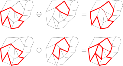
Figure 1: (a) Summation of two cycles resulting in a new cycle. Edges contained in either addend are contained in the sum. Edges present in both addends (dashed lines) cancel out. (b) Example of a sum of two cycles that is not a cycle itself.

We approximate the cycle length distribution by a Monte Carlo algorithm that considers cycles as discrete microstates of a physical system. Elementary transitions between cycles, the analogues of single spin flips in a spin system, are defined as addition or removal of short detours with minimal change to cycle length. By considering cycle length as energy, generic Monte Carlo procedures from statistical mechanics become applicable. Temperature is defined in the usual way and allows to tune the sampling on preferably long or short cycles. After introducing the algorithm in detail, we test its accuracy for a set of networks where the cycle length distribution is directly accessible for comparison. We apply the algorithm to models of growing networks and find the growth exponent of the mean cycle length. Finally, we test scaling of the number of cycles in the growing Internet.

The formulation of the algorithm uses the following basic notions of cycle space. We treat a subgraph $X$ as the set of edges it contains. If $X$ is a cycle, the cardinality $|X|$ is the cycle length. The sum of two subgraphs $X$ and $Y$ is defined as $X\oplus Y=(X\cup Y)\setminus(X\cap Y)$, i.e. an edge is contained in the sum if it is in one of the addends but not in both. The sum $X\oplus Y$ of two cycles $X$ and $Y$ is again a cycle if $X$ and $Y$ intersect in a suitable way, see Fig. 1. We generate a Markov chain of cycles $(C_{0},C_{1},C_{2},\dots)$ as follows. The initial condition is the empty graph $C_{0}=\emptyset$ at $t=0$. At each step a cycle $S$ is drawn at random from a set $M$ of initially known cycles (the choice of $M$ is described below). If the proposal $C^{\prime}=C_{t}\oplus S$ is a cycle or the empty graph, it is accepted with probability

$$P_{\rm accept}=\min\{\exp[-\beta(|C^{\prime}|-|C_{t}|)],1\}~{}.$$ (1)

In case of acceptance we set $C_{t+1}=C^{\prime}$, otherwise $C_{t+1}=C_{t}$. This is the Metropolis update scheme Metropolis53 with inverse temperature $\beta$ and energy as cycle length. Subgraphs that are not cycles are treated as states with infinite energy $E=\infty$ if $\beta>0$ (or $E=-\infty$ if $\beta<0$, respectively), such that they are always rejected.

Throughout this paper, we take $M$ as the set of short (isometric) cycles of the given graph. A cycle $S$ is short if for all vertices $x$ and $y$ on $S$, a shortest path between $x$ and $y$ lies also in $S$. As a non-short cycle has at least one short-cut between two of its vertices, it can be decomposed into two shorter cycles that overlap on the short-cut. Typically for each non-short cycle $C$ one finds cycles $S$ and $C^{\prime}$ such that $S$ is short and $|C^{\prime}|<|C|$. Applying the decomposition recursively, one sees that every cycle $C$ occurs in a sequence $0,C_{1},C_{2},\dots$ with $C_{i}\oplus C_{i+1}\in M$ and $|C_{i}|<|C_{i+1}|$. Thus taking as the possible “moves” $M$ the set of short cycles not only ensures that every cycle can be reached (ergodicity). In this case, the resulting energy landscape does not have any local minima other than the unique global minimum, which is the empty graph at $E=0$. There are exceptional graphs where the decomposability does not hold for one particular cycle. The exceptions appear to be irrelevant for the applications here as our numiercal results remain unchanged when $M$ is expanded to include more and longer (non-short) cycles.

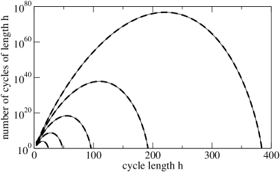
Figure 2: Number $c(h)$ of cycles of length $h$ estimated by the MC sampling algorithm (thick dashed curves) and the exact values from iterating Eq. (2) (thin solid curves). Studied networks are generations $n=4,\dots,8$ (system sizes $N=42,123,366,1095,3283$ vertices) from the deterministic growth model DorogovtsevReview . Given a network, a histogram is generated for each inverse temperatures $\beta\in[-5.0,\dots,+3.0]$ in steps of $\Delta\beta=0.1$. Each histogram is based on the lengths of the last $10^{8}$ cycles of a Markov chain of total length $2\times 10^{8}$. Then histograms are merged by choosing relative normalization such that the sum of squares of deviations in the overlapping region of adjacent histograms are minimized. The normalization of the final histogram is chosen such that $c(0)=1$. Results are robust against variation of the chain length.

Let us first test the algorithm on a set of networks where exact computation of $c(h)$ is feasible. The pseudo-fractal scale-free web by Dorogovtsev and Mendes Dorogovtsev02 grows deterministically by iterative triangle formation as follows. Start at generation $n=0$ with two vertices connected by an edge. To obtain generation $n+1$, for each edge $xy$ present in generation $n$ add a new vertex $z$ and the edges $xz$ and $yz$, such that each existing edge $xy$ becomes part of an additional triangle $xyz$. The calculation of $c(h)$ is particularly simple because each cycle has a unique predecessor in the previous generation, given by following direct links $xy$ instead of the additional “detours” via $z$. A cycle of length $h$ in generation $n$ produces $2^{h}$ cycles in generation $n+1$ as the result of $h$ binary decisions to follow the detour or the original direct edge. The histogram of cycle lengths iterates as

$$c^{(n+1)}(h)=\sum_{l=3}^{h}{h\choose h-l}c^{(n)}(l)$$ (2)

for $l\geq 4$ and $c^{(n+1)}(3)=c^{(n)}(3)+3^{n}$. The result of the numerical iteration of these equations up to generation $n=8$ is shown in Fig. 2, together with the results from the Monte Carlo method. The relative deviation of the sampling estimate of $c^{(n)}(h)$ from the exact value is below $25\%$ for all cycle lengths $h$ and all generations $n$. In particular, the unique cycle of maximum length $h_{\rm max}=3\times 2^{n}$ is detected. The method approximates the true numbers of cycles with large precision.

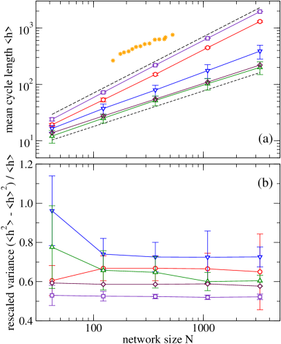
Figure 3: System size dependence of the cycle length distribution in growing networks. (a) Mean cycle length for the four stochastic attachment rules ($\Box,\bigcirc,\nabla,\triangle$) and the deterministic attachment rule ($\diamondsuit$). For the Internet ($\ast$), system size $N$ has been rescaled by factor 20 to fall into the displayed range. Dashed straight lines indicate growth exponents 1 and $\ln 2/\ln 3\approx 0.63$ for comparison. (b) Relative variance of the cycle length distribution for the same networks (same symbols as in (a)). In both panels, data points the stochastic growth models are averages over 10 network realizations each. Error bars indicate standard deviation over realizations.

Table 1: Networks with different attachment rules and the resulting scaling exponents $\gamma$ for the tail of the degree distribution and $\alpha$ for the growth of the cycle lengths. The last column displays the symbol used in Fig. 3.

rule	indep / tri	hom / pref	$\alpha$	$\gamma$
IH Barabasi99	independent	homogeneous	$1.010(4)$	$\infty$	$\Box$
IP Barabasi99	independent	preferential	$0.969(5)$	$3$	$\bigcirc$
TH	triangle	homogeneous	$0.722(5)$	$\infty$	$\nabla$
TP Dorogovtsev01	triangle	preferential	$0.644(9)$	$3$	$\triangle$
PF Dorogovtsev02	triangle	preferential	$0.635(1)$	$2.59$	$\diamondsuit$
Internet			$0.76(4)$	$2.22(1)$	$\ast$

Now we apply the algorithm to study the system size dependence of the cycle length distribution of stochastically growing artificial networks. All networks initiate as two vertices coupled by an edge. The networks grow by iterative attachment of vertices until a desired size $N$ is reached. At each iteration, one new vertex $z$ and two new edges $xz$ and $yz$ are generated. We are interested in the influence different attachment mechanisms have on the cycle length distribution. Therefore we distinguish four probabilistic rules for selection of the nodes $x$ and $y$ to which the new node $z$ attaches. Independent homogeneous (IH) attachment: Draw $x$ and $y$ randomly (with equal probabilities) and independently from the set of nodes; if $x=y$, discard this choice and repeat. Independent preferential (IP) attachment: Draw an edge randomly (all edges having equal probability) and take as $x$ one of the end vertices chosen with equal probability; draw another edge to find $y$ analogously; if $x=y$, discard this choice and repeat. Triangle forming preferential (TP) attachment: Draw an edge randomly and take its two end vertices as $x$ and $y$. Triangle forming homogeneous (TH) attachment: Draw an edge randomly, take $x$ and $y$ as its end vertices and accept this choice with probability $1/(\deg(x)\deg(y))$; otherwise reject and repeat.

Rule IP is equivalent to choosing nodes with probability proportional to degree Barabasi99 , so-called preferential attachment. It generates scale-free networks with degree exponent $\gamma=3$. Rule TP implements preferential attachment with the additional constraint that $x$ and $y$ be connected; it is the stochastic version of the pseudo-fractal (PF) scale-free web Dorogovtsev01 defined above. The resulting networks are scale-free with $\gamma=3$. The homogeneous attachment rule (IH) Barabasi99 leads to networks with exponentially decaying degree distribution ($\gamma=\infty$). The fourth rule (TH) introduced here combines triangle formation with homogeneous attachment by explicitly canceling out the degree dependence in the selection probability. We have checked that this rule generates an exponential degree distribution.

As shown in Fig. 3(a) the mean cycle length increases algebraically with system size,

$$\langle h\rangle\sim N^{\alpha}~{},$$ (3)

with the exponent $\alpha\in[0,1]$ depending on the attachment rule. The variance of the cycle length distribution increases algebraically with the same exponent $\alpha$. Therefore the ratio between variance and mean is practically constant, see Fig. 3(b). Considering the degree exponent $\gamma$ and the cycle growth exponent $\alpha$ for each type of network (Table 1), several observations are worth mentioning. Homogeneous attachment with triangle formation leads to a non-trivial cycle growth exponent $\alpha\approx 0.72$ even in the absence of scaling in the degree distribution $\gamma=\infty$. Networks grown stochastically with triangle formation and preferential attachment (rule TP) have the same exponent $\alpha\approx 0.64$ as the deterministic counterpart (rule PF) while the degree exponents under these two rules are clearly different. Analogously, in the absence of triangle formation (rules IH and IP) the same cycle growth exponent $\alpha\approx 1.0$ is obtained regardless of the degree exponents $\gamma\in\{3,\infty\}$.

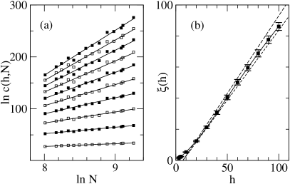
Figure 4: Evolution of cycles in the growing Internet at the Autonomous Systems level. (a) The number of cycles of given length $h$ as a function of system size $N$ for $h=10,20,30,\dots,100$ (squares, bottom to top). The straight lines are best fits of the form $c(h,N)\propto N^{\xi(h)}$. (b) Growth exponents $\xi(h)$ as defined in Eq. (4) obtained as slopes of the fitted lines in (a). Error bars of exponents indicate standard error from the fit. Dashed lines have slopes $1.0$ and $0.9$.

Finally we consider cycles in an evolving real-world network. The Internet at the level of Autonomous Systems is a growing scale-free network with degree exponent $\gamma=2.22(1)$ Faloutsos99 ; Pastor01b . Here we analyze snapshots of the network with sizes from $N=3015$ nodes (November 1998) to $N=10515$ nodes (March 2001) InternetData . We find that during this time the mean cycle length grows from 264.9 to 757.8, as plotted in Fig. 3(a). As in the artificial growing networks, the growth is algebraic. The growth exponent is estimated as $\alpha=0.76(4)$ by a least squares fit. More detailed analysis is performed on the number $c(h,N)$ of cycles of given length $h$ at system size $N$ plotted in Fig. 4(a). We observe a scaling

$$c(h,N)\sim N^{\xi(h)}~{}.$$ (4)

with an exponent $\xi(h)$ that depends linearly on $h$ with a slope close to unity. Figure 4(b) shows that

$$\xi(h)\approx h~{}.$$ (5)

for not too small lengths $h\geq 10$. The scaling behavior is in qualitative agreement with the prediction from the first order approximation by Bianconi et al. Bianconi05b , assuming that the Internet is a random network with a given scale-free degree distribution.

In summary, we have introduced a method for sampling cycles in large graphs. We have identified cycle space with the state space of a system with many degrees of freedom, thereby making Monte Carlo techniques from statistical mechanics applicable. In this framework, we have analyzed the evolution of cycles in growing networks. While the mean cycle length grows with a characteristic exponent $\alpha$ the relative width of the length distribution tends to zero as the system size increases. Thus, in agreement with an earlier speculation Rozenfeld05 , the exponent $\alpha$ is found to be the most relevant quantity for the evolution of cycle space. In the scale-free model by Barabási and Albert Barabasi99 as well as the growth model with random homogeneous attachment, cycles are space-filling ($\alpha=1.0$), i.e. cycle length is proportional to system size. In model networks with explicit formation of triangles and in the Internet, however, cycles grow slower than the system as a whole. This class of networks having $\alpha<1$ also includes single-scale networks with $\gamma=\infty$. Our study suggests that the cycle growth exponent may serve as a characterization of growing networks independent of the degree exponent $\gamma$. An open question concerns universality. Can $\alpha$ be altered continuously by tuning parameters or does it assume distinct values, separating growing networks into universality classes?

We are grateful to C. P. Bonnington, J. Leydold, and A. Mosig for inspiring discussions. This work was supported by the DFG Bioinformatics Initiative BIZ-6/1-2.

References

- (1) R. Albert, A.-L. Barabási, Rev. Mod. Phys. 74, 47 (2002).
- (2) S. N. Dorogovtsev, J. F. F. Mendes, Adv. Phys. 51, 1079 (2002).
- (3) S. Bornholdt and H. G. Schuster (Eds.), Handbook of Graphs and Networks - From the Genome to the Internet Wiley-VCH, Berlin (2002).
- (4) C. Song, S. Havlin, and H. A. Makse, Nature 433, 392 (2005)
- (5) E. Ravasz and A.-L. Barabási, Phys. Rev. E 67, 026112 (2003)
- (6) A.-L. Barabási and R. Albert, Science 286, 509 (1999).
- (7) R. Pastor-Satorras and A. Vespignani, Phys. Rev. Lett. 86, 3200 (2001).
- (8) R. Albert R, H. Jeong, A.-L. Barabási Nature 406, 378 (2000).
- (9) D. J. Watts and S. H. Strogatz, Nature 393, 440 (1998).
- (10) G. Bianconi and A. Capocci, Phys. Rev. Lett. 90, 078701 (2003).
- (11) E. Marinari, and R. Monasson, J. Stat. Mech. P09004 (2004).
- (12) E. Ben-Naim and P. L. Krapivsky, Phys. Rev. E 71, 026129 (2005).
- (13) A. Vázquez, J. G. Oliveira, and A.-L. Barabási, Phys. Rev. E 71, 025103(R) (2005).
- (14) G. Bianconi, M. Marsili, cond-mat/0502552 (2005).
- (15) H. D. Rozenfeld, J. E. Kirk, E. M. Bollt, and D. ben-Avraham, J. Phys. A.: Math. Gen. 38, 4589 (2005).
- (16) N. Metropolis et al., J. Chem. Phys. 21, 1087 (1953).
- (17) S. N. Dorogovtsev, A. V. Goltsev, and J. F. F. Mendes, Phys. Rev. E 65, 066122 (2002).
- (18) S. N. Dorogovtsev, J. F. F. Mendes, and A. N. Samukhin, Phys. Rev. E 63 062101 (2001).
- (19) http://www.cosin.org
- (20) M. Faloutsos, P. Faloutsos, and C. Faloutsos, Comput. Commun. Rev. 29, 251 (1999).
- (21) R. Pastor-Satorras, A. Vázquez, and A. Vespignani Phys. Rev. Lett. 87, 258701 (2001)
- (22) Ginestra Bianconi, Guido Caldarelli, and Andrea Capocci, Phys. Rev. E 71, 066116 (2005).