Knudsen Effect in a Nonequilibrium Gas

Abstract

From the molecular dynamics simulation of a system of hard-core disks in which an equilibrium cell is connected with a nonequilibrium cell, it is confirmed that the pressure difference between two cells depends on the direction of the heat flux. From the boundary layer analysis, the velocity distribution function in the boundary layer is obtained. The agreement between the theoretical result and the numerical result is fairly good.

Although there has been a long history of nonequilibrium statistical mechanics since Boltzmann introduced the Boltzmann equation, the understanding of nonequilibrium statistical mechanics is still in the primitive stages [1, 2, 3]. The significant role of nonequilibrium physics in the mesoscopic region has been recently recognized. For example, there has been some important progress such as the Fluctuation Theorem [4, 5] and the Jarzynski equality [6] in mesoscopic nonequilibrium statistical mechanics. In typical situations of mesoscopic physics, materials are confined to narrow regions. Thus the boundary effects at the mesoscopic scale are important not only for nonequilibrium statistical mechanics but also for consideration of friction and lubrication [7].

On the other hand, some macroscopic phenomenologies for nonequilibrium steady states have been proposed. These are the Extended Thermodynamics (ET) [8], the Extended Irreversible Thermodynamics (EIT) [9, 11, 10] which is the combination of ET and information theory, and the Steady State Thermodynamics (SST) [12]. It is interesting that both EIT and SST treat a common process in which a nonequilibrium cell is connected with an equilibrium cell [12, 11].

The Knudsen effect is the phenomenon in which two equilibrium cells with different temperatures are connected by a small hole [3]. The balance equation of the Knudsen effect is given by

$$\frac{P_{1}}{\sqrt{T_{1}}}=\frac{P_{2}}{\sqrt{T_{2}}},$$ (1)

where $T_{i}$ and $P_{i}$ represent the temperature and the pressure in the cell, $i$, respectively. Although eq. (1) contains only macroscopic variables, it is in contrast to the ordinary thermodynamic balance condition where the pressures the two cells are equal. Such an exceptional condition means that the mass balance is determined by the transportation of the gases in the small hole. Therefore, the relevance of predictions by macroscopic theory [10, 12] for the generalized Knudsen effect in which an equilibrium cell is connected with a nonequilibrium cell by a small hole is questionable.

On the other hand, the explicit perturbative solution of the Boltzmann equation for hard spheres has been derived at the Burnett order of the heat flux [13, 14]. The quantitative accuracy and numerical stability of their solution in the bulk region has been confirmed by molecular dynamics (MD) simulation for hard-spheres [15] and the extension to the tenth order shows that their second order solution is accurate even when the heat current is large [16]. They have confirmed that the solution in the bulk region derived by information theory is not consistent with that of the Boltzmann equation [17]. Kim and Hayakawa [13] have also discussed the nonequilibrium Knudsen effect. Their result denies the prediction of SST, but both theories predict that the osmosis $\triangle P$ defined by the $\triangle P\equiv P_{xx}^{neq}-P^{eq}$ with the $xx$ component of the pressure tensor $P_{xx}^{neq}$ in the nonequilibrium cell and the pressure $P^{eq}$ in the equilibrium cell is always positive regardless of the direction of heat flux.

However, their simplification [13] using the bulk solution of the Boltzmann equation in the boundary layer is not acceptable. In fact, numerical simulations of the Boltzmann equation of hard spheres [18] exhibit the discontinuity of velocity distribution function (VDF) in the boundary layer, but there is no discontinuity of VDF derived by Kim and Hayakawa [13, 14]. Furthermore, it is also well known that the gas temperature near the wall is different from the wall temperature [18, 3, 2, 19], but both treatments [12, 13] ignore this fact.

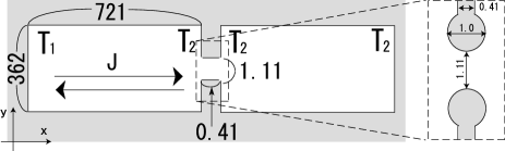
Figure 1: The schematic picture of the system of our simulation, where the right cell is at equilibrium with temperature $T_{2}$ and the left cell is in a nonequilibrium state. The inset represents the detailed structure of the hole that has the gap $1.11$. The unit of length in figures is the diameter of the rigid disk. We adopt periodic boundary condition in the $y$ direction.

To clarify the truth of the nonequilibrium Knudsen effect, we employ the event-driven molecular dynamics simulation of hard-disks developed in refs. [20-23]. Let $x$ and $y$ be the Cartesian coordinates of the horizontal and the vertical directions, respectively. First we check the validity of eq. (1) by MD. We adopt the diffusive reflection for the vertical walls away from the hole, the simple reflection rule for the wall between two cells and the periodic boundary condition for the horizontal wall. We connect two cells by a small hole, as illustrated in Fig. 1. For $T_{1}/T_{2}=1.96$, we have found the steady value of $P_{1}/P_{2}\sqrt{T_{2}/T_{1}}=0.9982\pm 0.0195$, where the average area fraction and the number of the particle are $0.015$ and $10,000$ respectively. We determine the pressure based on the Virial theorem [24] and average in $10^{4}$ collisions per particle. The stationary state is realized after $3\times 10^{5}$ collisions per particle and we use the data after that. We simulate the system until $10^{6}$ collisions have been performed per particle.

Next, we simulate the nonequilibrium Knudsen effect. The number of hard disks and the average area fraction are the same values used to simulate the conventional Knudsen effect. We adopt the diffusive boundary condition for the wall between two cells (see Fig. 1). We examine the values of $T_{1}/T_{2}$ as $1.96$ and $1/1.96$. We cause both cells to divide into 10 equal parts, and we have confirmed that pressure based on the Virial theorem [24] is identical in each cell. This is consistent with the stationary condition [19]. In nonequilibrium cases the stationary state is realized after $10^{6}$ collisions per particle and we use the data after that. We simulate the system until $4.4\times 10^{6}$ collisions have been performed per particle.

Our results of MD plotted in Fig. 2 indicate that the sign of $\triangle P(\equiv P^{neq}_{xx}-P^{eq})$ depends on the direction of energy flux. Actually, the stationary value $\triangle P$ in our simulation is given by $\triangle P/<n_{2}T_{2}>=0.0279\pm 0.0184$ for $T_{1}/T_{2}=1.96$, and $\triangle P/<n_{2}T_{2}>=-0.0152\pm 0.0175$ for $T_{1}/T_{2}=1/1.96$, where $<n_{2}T_{2}>$ is the time average of $n_{2}T_{2}$ (Fig. 2). This result contrasts with the positive $\triangle P$ predicted by both SST [12] and Kim and Hayakawa [13].

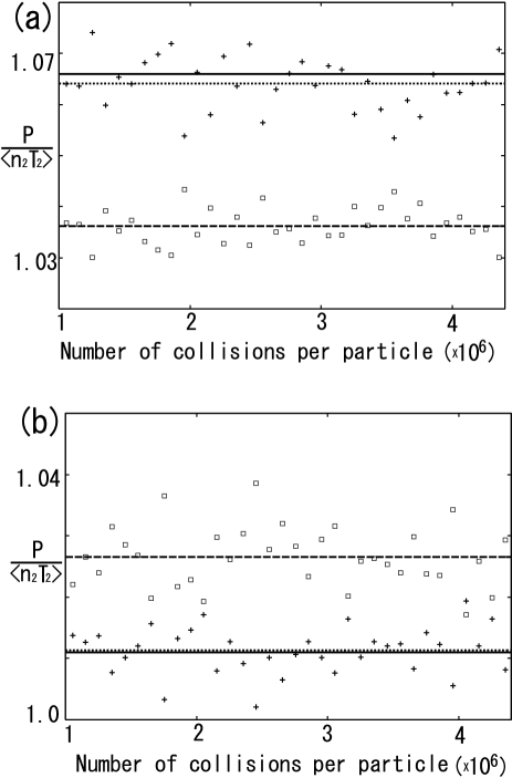
Figure 2: The time dependence of the pressure for (a) $T_{1}/T_{2}=1.96$ and (b) $T_{1}/T_{2}=1/1.96$. Here $P^{neq}_{xx}$ in the nonequilibrium cell is plotted by plus points and its time average is shown by the dotted line. In each case the pressure $P^{eq}$ in the equilibrium cell is plotted by open square points and its time average is plotted by the dashed line. The theoretical $P^{neq}_{xx}$ in eq. (11) is shown by the solid line. For the normalization, we divide these values by $<n_{2}T_{2}>$.

Now let us compare the VDF of MD with the perturbative solution of the Boltzmann equation at the Burnett order obtained by Kim [14] for 2D hard disks. From now on, we restrict our interest to the data for heat flux $J<0$, with $T_{1}/T_{2}=1/1.96$. As shown in Fig. 3, VDF obtained from MD in the bulk region of a nonequilibrium cell is almost identical to the theoretical VDF, where the VDF of MD is obtained from the average of particles existing in $\pm 1.05d$ from the center of nonequilibrium cell in the horizontal direction with hard disk diameter $d$. On the other hand, the VDF in the boundary layer in which we average the data of particles existing between $0.7d$ and $2.8d$ apart from the right wall of the nonequilibrium cell deviates from the theoretical VDF [14], particularly for $v_{x}<0$ (Fig. 4).

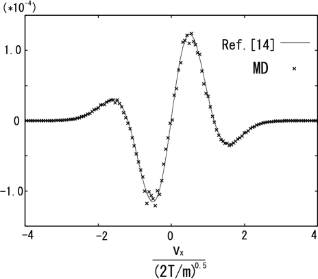
Figure 3: Comparison of VDFs derived by simulation and Ref.[14] at the middle of the nonequilibrium cell. The plotted data are the substraction of Maxwellian from VDFs.

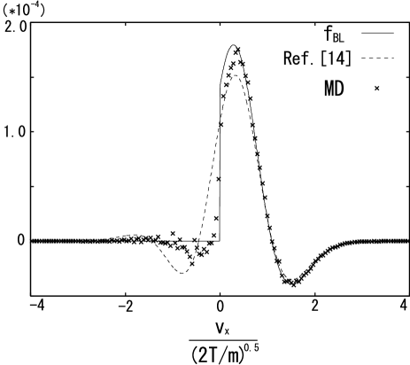
Figure 4: Comparison of VDFs derived by simulation and Ref.[14] and $f_{BL}$ in eq. (2) at the near the wall. The plotted data are the substraction of Maxwellian from VDFs.

Let us derive VDF in the boundary layer in the nonequilibrium cell. We assume that the VDF of the incident particles ($v_{x}>0$) in the boundary layer is the same as the bulk distribution function ($f_{NE}$). On the other hand, we assume that the VDF for the particles reflected by the wall ($v_{x}<0$) obey the Maxwellian.

Thus, the distribution function $f_{BL}$ in the boundary layer is given by

$$f_{BL}({\bf v})=\begin{cases}f_{MB}(n_{w},T_{w},{\bf v})&v_{x}<0\\ f_{NE}(n_{x},T_{x},J,{\bf v})&v_{x}\geq 0,\end{cases}$$ (2)

where

$$f_{MB}(n_{w},T_{w},{\bf v})\equiv\frac{n_{w}m}{2\pi T_{w}}\exp{\left[-\frac{m{\bf v}^{2}}{2T_{w}}\right]},$$ (3)

with the mass of a hard-disk $m$, and

$$\begin{split}f_{NE}(n_{x},T_{x},J,&{\bf v})\equiv f_{MB}(n_{x},T_{x},{\bf v})\times\\ &\left[1-\frac{mJv_{x}}{2b_{1}n_{x}T_{x}^{2}}\sum_{r\geq 1}r!b_{r}L^{1}_{r}\left(\frac{m{\bf v}^{2}}{2T_{x}}\right)\right],\end{split}$$ (4)

with $b_{1}=1.03,b_{2}=5.738\times 10^{-2},b_{3}=4.946\times 10^{-3},b_{4}=4.313\times 10^{-4},b_{5}=3.452\times 10^{-5},b_{6}=2.241\times 10^{-6}$ and Laguerre’s bi-polynomial $L^{a}_{b}(x)$ [14]. Since the heat flux is sufficiently small, we adopt the first order nonequilibrium VDF in the heat-flux for $f_{NE}$.

There are three unknown variables, $n_{w}$, $n_{x}$, and $T_{x}$ in eqs. (3) and (4), while there are three relations,

$$n \equiv\int d{\bf v}\,f_{KL}({\bf v}),$$ (5)

$$J \equiv m\int d{\bf v}\,v_{x}\frac{{\bf v}^{2}}{2}f_{KL}({\bf v}),$$ (6)

$$\int d{\bf v}\,v_{x}f_{KL}({\bf v})=0.$$ (7)

Here, the first two equations are definitions of the density $n$ and the heat flux $J$, and the last equation represents the mass balance condition. Therefore, we can determine $n_{w}$, $n_{x}$, and $T_{x}$ from eqs. (5)-(7). The expansions in terms of $J$ of the three variables become

$$n_{w}=n+a\frac{m^{1/2}}{T_{w}^{3/2}}J,$$ (8)

$$n_{x}=n+b\frac{m^{1/2}}{T_{w}^{3/2}}J,$$ (9)

$$T_{x}=T_{w}+c\frac{m^{1/2}}{nT_{w}^{1/2}}J,$$ (10)

where $a$, $b$ and $c$ are constants to be determined. From eqs. (5),(6) and (7), we obtain the solutions of the linear simultaneous equations as $(a,b,c)\simeq(0.32,-0.099,0.84)$.

The distribution function $f_{BL}$ near the wall has thereby been determined by $n,T_{w}$, and $J$. Figure 4 is the comparison of $f_{BL}$ with the results of MD. From Fig. 4, both $f_{BL}$ and the VDF from MD have a discontinuity at $v_{x}=0$, as in the case of conventional boundary layer analysis [18]. For reflective VDF ($v_{x}<0$), there is the small difference between the result of MD and the Maxwellian. We may deduce that it arises from collisions between particles because we measure the VDF a short distance from the wall.

With the aid of $f_{BL}$, $\triangle P$ can be calculated as

$$\triangle P\simeq\frac{-a+b+c+0.412}{2}\frac{J}{\sqrt{T_{2}}}=0.415\frac{J}{\sqrt{T_{2}}}.$$ (11)

From this equation and the value of the heat-flux in MD, we evaluate $\triangle P/<n_{2}T_{2}>\simeq 0.0298$ for $T_{1}/T_{2}=1.96$ and $\triangle P/<n_{2}T_{2}>\simeq-0.0156$ for $T_{1}/T_{2}=1/1.96$. The result agrees well that of the simulation. We can also obtain the temperature jump coefficient $\gamma\simeq 0.97$ which is defined through $T_{x=0}-T_{w}=\gamma J/n\sqrt{m/T_{w}}$.

Now, let us discuss our result. There are some advantages to employing MD as the numerical simulation. First, we can easily change boundary conditions for walls depending on our interest. The system of connecting two cells by a small hole is easily simulated by MD. Second, MD is suitable for high density simulation of gases. The nonequilibrium Knudsen effect for high density gases is an interesting subject for future discussions. We are also interested in the size effect of the hole on the transition from Knudsen balance to the thermodynamic balance. On the other hand, there are some disadvantages to employing MD. Because of the small system size of our MD simulation, the fluctuation of the pressure is large.

The advantage of our boundary layer analysis is that we can write the explicit form of VDF in the boundary layer in terms of the density, the heat-flux and the temperature of the wall. On the other hand, VDF by Sone et al [18] has an implicit form that is obtained as a numerical solution of an integral equation. The explicit VDF can be obtained by our simplification, but the validity of this method has not been confirmed. In fact, for 3D hard-sphere gases, our method predicts the temperature jump coefficient $\gamma\simeq 0.72$, while Sone et al [18] predicts $\gamma\simeq 1.00$. To check the validity of our boundary layer analysis, it will be necessary to employ 3D MD simulation for 3D.

We also stress the difficulty of describing the nonequilibrium Knudsen effect by macroscopic phenomenology. In fact, our boundary layer analysis strongly depends on the boundary condition.

In conclusion, the sign of $\triangle P$ depends on the direction of the heat flux. The approximated VDF in the boundary layer has been obtained from the assumption that the incident particles obey the bulk VDF and the reflected particles obey the Maxwellian. This agrees well with the simulation result.

The authors would like to thank M. Fushiki and H.-D. Kim for their valuable comments. They appreciate Aiguo Xu for his critical reading of the manuscript. This work is partially supported by a Grant-in-Aid from the Japan Space Forum and the Ministry of Education, Culture, Sports, Science and Technology (MEXT), Japan (Grant No. 15540393) and a Grant-in-Aid from the $21$st century COE “Center for Diversity and Universality in Physics” from MEXT, Japan.

References

- [1] S. Chapman and T. G. Cowling: The Mathematical Theory of Non-uniform Gases (Cambridge University Press, London, 1970)
- [2] Y. Sone: Kinetic Theory and Fluid Dynamics (Birkhäuser, Boston, 2002)
- [3] E. M. Lifshitz and L. P. Pitaevskii: Physical Kinetics, (Pergamon Press, Oxford, 1981)
- [4] D. J. Evans, E. G. D. Cohen, and G. P. Morriss: Phys. Rev. Lett. 71 (1993) 2401.
- [5] D. J. Evans and D. J. Searles: Advances in Physics 51 (2002) 1529.
- [6] C. Jarzynski: Phys. Rev. Lett. 78 (1997) 2690.
- [7] S. Granick: Physics Today 52 7 (1999) 26.
- [8] I. Müeller and T. Ruggeri: Extended Thermodynamics, (Springer, Berlin, 1993).
- [9] D. Jou, J. Casas-Vázquez, and G. Lebon: Rep. Prog. Phys. 51 (1988) 1105.
- [10] R. Dominguez and D. Jou: Phys. Rev. E 51 (1995) 158.
- [11] D. Jou, J. Casas-Vázquez, and G. Lebon: Extended Irreversible Thermodynamics, (Springers,2001).
- [12] S. Sasa and H. Tasaki: cond-mat/0411052.
- [13] H.-D. Kim and H. Hayakawa: J. Phys. Soc. Jpn 72 (2003) 1904. [Erratum: 73 (2004) 1609]
- [14] H.-D. Kim: Phys. Rev. E 71 (2005) 041203.
- [15] M. Fushiki: unpublished.
- [16] M. Fushiki: submitted to Phys. Rev. Lett..
- [17] H.-D. Kim and H. Hayakawa: J. Phys. Soc. Jpn. 72 (2003) 2473.
- [18] Y. Sone, T. Ohwada, and K. Aoki: Phys. Fluids A 1 (1989) 363. [Erratum: 1 (1989) 1077]
- [19] P. Welander: Ark. Phys. 7 (1954) 507.
- [20] D. C. Rapaport: J. Comp. Phys. 34 (1980) 184.
- [21] M. Marín, D. Risso and P. Cordero: J. Comp. Phys. 109 (1993) 306.
- [22] M. Marín and P. Cordero: Comp. Phys. Commu. 92 (1995) 214.
- [23] M. Isobe: Int. J. Mod. Phys. C10 7 (1999) 1281.
- [24] D. J. Evans and G. P. Morris: Statistical Mechanics of Nonequilibrium Liquids (Academic Press, London, 1990)