Electronic and magnetic properties of a hexanuclear ferric wheel

Abstract

The electronic and magnetic properties of the hexanuclear ferric wheel [LiFe₆(OCH₃)₁₂-(dbm)₆]PF₆ have been studied with all-electron Hartree-Fock and full-potential density functional calculations. The best agreement for the magnetic exchange coupling is at the level of the B3LYP hybrid functional. Surprisingly, the Hartree-Fock approximation gives the wrong sign for the exchange coupling. The local density approximation and the gradient corrected functional PBE strongly overestimate the exchange coupling due to the too large delocalization of the $d$-orbitals. These findings are supported by results from the Mulliken population analysis for the magnetic moments and the charge on the individual atoms.

I Introduction

Molecular magnetism has received great attention in the past few years, especially after a series of molecules has been discovered which show magnetism due to a molecular origin (see the review articlescaneschi1999 ; pilawa1999 ). One particular type of molecular magnets are the so-called ferric wheels where iron atoms are arranged ring-like. So far, wheels with 6 up to 18 iron atoms have been synthesizedcaneschi1999 . This has also triggered interest among theorists. The description of magnetism still poses challenges, and only in the last years ab-initio calculations of large molecular magnets have become feasible postnikovpsik .

The early studies employed wave-function based methods: for example, the exchange interaction in transition metal oxides was investigated at the level of periodic Hartree-Fock calculations Towler1994 . Usually, it is found that the Hartree-Fock approximation strongly underestimates the exchange coupling (e.g. Towler1994 ; ricart1995 ; catti1995 ). This was also demonstrated for smaller molecules, where demanding configuration interaction calculations were feasible: it was shown, that for a proper description of the magnetic interactions, highly correlated wave functions are necessaryFink1 ; Fink2 .

With the help of an appropriate embedding, the bulk could be approximatively described with clusters. Then, wave-function based correlation methods could be applied and a value in reasonable agreement with the experimental value of the exchange coupling was deduced degraaf ; moedl .

In the past few years, density functional calculations have become more and more widespread, and have also been applied to molecular magnets (e.g. postnikovpsik ; ruiz2003 ; zeng1 ). They have the advantage of including approximatively the effects of electronic correlation, at a very low computational expense. However, it is often observed that exchange couplings, computed at the density functional level (especially the local density approximation), strongly overestimate the experimental value. In a comparative study, it was shown that hybrid functionals, which include the exact (Fock) exchange, improve this and provide surprisingly accurate values iberio . This was also observed earlier in cluster calculations which were used to model the solid MartinIllas1997 .

The ferric wheel with six iron atoms is one of the smaller molecular magnets and thus ab-initio calculations can be performed at a relatively low expense, besides the approach using model Hamiltonians Normand ; Honecker . Various molecules have been synthesized Caneschi1995angew ; Caneschi1996 ; Abbati1997 ; Lascialfari1997 ; Pilawa1997 ; Saalfrank1997 ; Waldmann1999 ; Affronte1999 ; Cornia1999 ; Affronte2002 ; Pilawa2003 and techniques such as nuclear magnetic resonance, high-field DC and pulsed-field differential magnetization experiments, susceptibility measurements, high field torque magnetometry, inelastic neutron scattering and heat capacity measurements have been applied.

The experimental values for the exchange couplings, extracted from susceptibility measurements or from the singlet-triplet gap, are typically around $\sim$20 K caneschi1999 ; Waldmann1999 ; Cornia1999 ; Affronte1999 ; Pilawa2003 , although also larger values have been suggested (e. g. 38 KLascialfari1997 ). As there are still only few ab-initio calculationspostnikov2003 ; postnikov2004 , these systems are therefore an interesting object to study.

This article will deal with one of the six-membered iron ferric wheels Abbati1997 . In previous studies on a similar system with a gradient corrected functional, an overestimation of the calculated exchange coupling by a factor of $\sim$ 4 was found and it was argued that schemes such as LDA+$U$ or self-interaction correction might resolve this problempostnikov2003 ; postnikov2004 . As was argued above, hybrid functionals might be a different way to deal with this problem. We therefore studied this ring at the level of various functionals including hybrid functionals, and the traditional Hartree-Fock approach.

II Method

All the calculations were done with the code CRYSTAL2003 crystal ; dovesi . We employed the Hartree-Fock (HF) method (in the variant of unrestricted Hartree-Fock), the local density approximation (LDA) with the correlation functional of Perdew and ZungerPZ , the gradient corrected functional of Perdew, Burke and Ernzerhof (PBE)PBE and the hybrid functional B3LYP (a functional with admixtures, amongst others, of functionals by Becke, Lee, Yang and Parr). As described later on in this section, we performed the calculations mainly on a molecular system. Therefore, we also used a basis set library for molecular basis setsBasistext rather then the CRYSTAL basis set library which contains essentially basis sets for periodic systems. We chose a [5s4p2d] basis set for iron Fe , where the diffuse exponent 0.041148 was omitted, a [2s] basis set for hydrogenditchfield , a [3s2p] basis set for carbonhehre where the exponent 0.1687144 was replaced with 0.25 to avoid convergence problems, a [3s2p] basis set for oxygenoxy with an additional $d$-exponent of 0.8 and a [3s2p] basis set for lithium oxy where the exponent 0.2 was omitted. After the mentioned modifications, the final basis sets were thus of the size [4s3p2d] (iron), [3s2p] (carbon), [3s2p1d] (oxygen), [2s] (hydrogen) and [2s1p] (lithium).

To explore the influence of further basis functions, various tests were performed: calculations with an additional $sp$-shell (exponent 0.04) and an additional $d$-shell (exponent 0.2) at the iron atom have been carried out, at the B3LYP and HF level. Also calculations with an additional $sp$-shell (exponent 0.12) at the oxygen atoms were performed at the B3LYP level. This diffuse exponent led to linear dependence problems at the HF level. However, a HF calculation where the outermost exponent 0.270006 for oxygen was replaced with two exponents (0.5, 0.2) was numerically stable. No significant changes for the computed exchange couplings were observed in any of these aforementioned tests. Therefore the basis sets, as described in the first paragraph of this section, can be considered reliable, and all the results were obtained with these basis sets, if not explicitly stated otherwise.

The properties of the ferromagnetic (FM) state (all spins parallel, total spin 30 $\mu_{B}$) and of the antiferromagnetic (AF) state (spins alternating up and down, total spin 0) were computed with each method. To obtain the local magnetic moments, a Mulliken population analysis was performed.

The calculations were performed on an isolated molecule where the full symmetry of the molecule was exploited (ferromagnet: $C_{3i}$, antiferromagnet: $C_{3}$). The geometry was chosen according to the measurements by Abbati et al Abbati1997 and is displayed in figure 1. The isolated molecule was charged with +1, as lithium is ionized and charge neutrality is restored by a PF${}_{6}^{-}$ ion for this particular ferric wheel. To assess the influence of the centered lithium ion it was also removed in some of the calculations.

III Results

The total energies, the difference in total energies of the ferromagnet and the antiferromagnet and the exchange parameters $J$ are given in table 4. To obtain the exchange parameters J from the calculation, the spin Hamiltonian of the Ising model was used:

$$\textbf{H}=-J\sum_{i=1}^{5}S_{i}\cdot S_{i+1}-J\cdot S_{6}\cdot S_{1}$$

The variable $i$ corresponds to the site index of the iron atoms, which in this model possess a spin of $S=5/2$. With this Hamiltonian, the energy difference between ferromagnet(FM) and antiferromagnet(AF) then corresponds to:

$$E_{tot}^{FM}-E_{tot}^{AF}=-12JS^{2}$$

Therefore, the exchange parameter J results from the difference of large numbers. Still the results are numerically stable, as can be seen in table 4. For the particular ferric wheel under consideration, the experimental value for the exchange coupling was determined to be -21 K Abbati1997 ; caneschi1999 .

This can now compared with the computed values. One interesting result is the ferromagnetic exchange parameter obtained at the Hartree-Fock level (+7 K ) which does not reproduce the real antiferromagnetic nature of the molecule. This result was stable $(\pm 2K)$ with respect to all possible variations in the basis set as mentioned in section II, and also when the central lithium ion was removed.

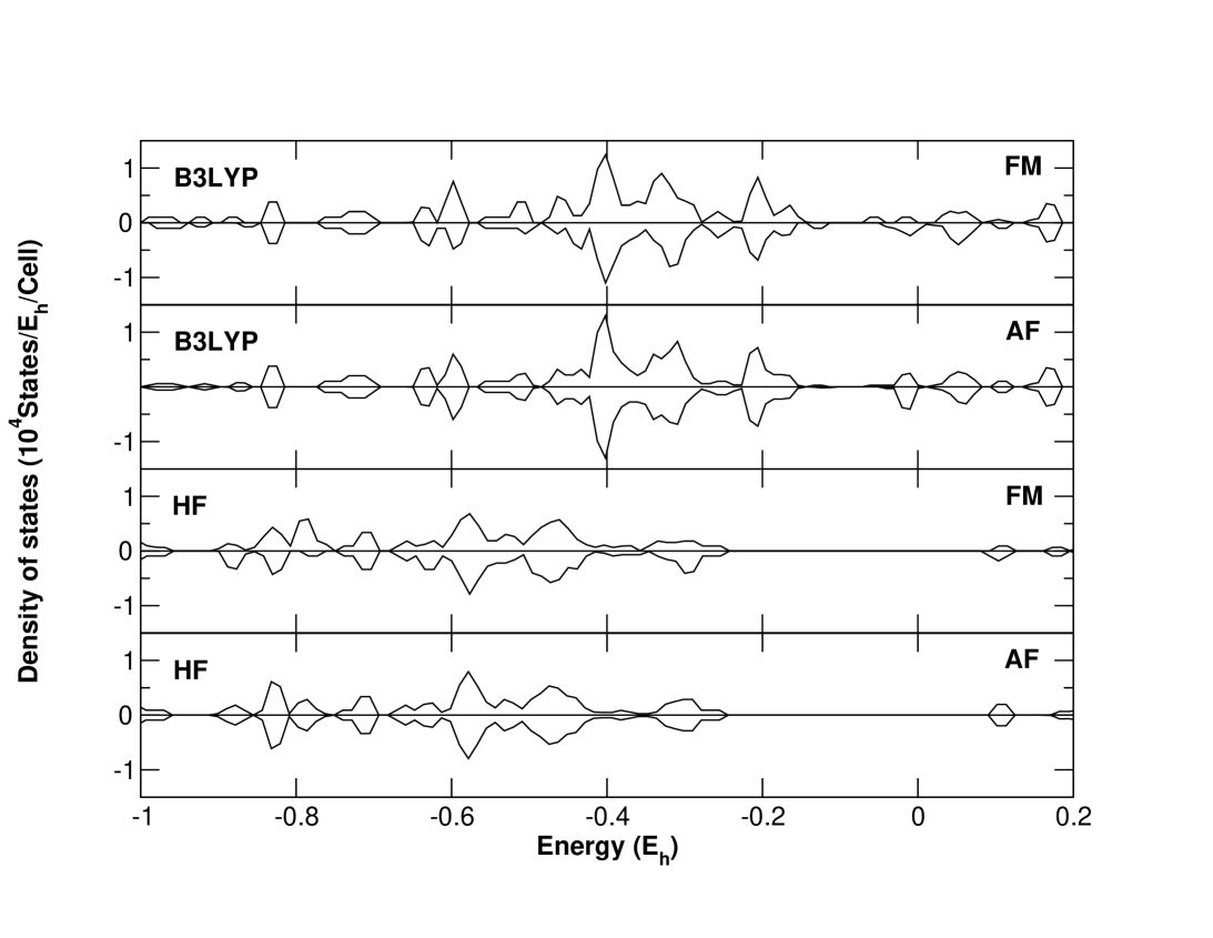
Figure 2: The total density of states for the ferromagnetic and antiferromagnetic state at the B3LYP level (upper two graphs) and the HF level (lower two graphs). For this purpose, the calculations had to be carried out as bulk calculations, with a lattice constant of 100 Å to avoid interactions between the molecules, and with the central lithium ion removed in order to have a non-charged unit cell. The top of the valence band is at -0.12 E_h (B3LYP) and at -0.26 E_h (HF).

Such a problem did not show up with any of the density functionals. The magnitude of $J$ of the B3LYP calculation (-31 K) is about 50$\%$ larger than the experimental value. In the PBE and LDA calculations, it is even overestimated by a factor of $\sim$ 5 (PBE: -108 K, LDA: -120 K). This agrees well with an earlier calculation for a similar ferric wheel by Postnikov et al postnikov2003 ; postnikov2004 with the PBE functional, where $J$ was also largely overestimated (-80 K). The authors argued, that the $d$-orbitals in density functional calculations with functionals such as LDA or PBE, were not sufficiently localized to compare with experiment, and therefore the resulting exchange parameters would overestimate the experimental values. They therefore suggested to use methods such as LDA+$U$ or self-interaction corrections to improve this shortcoming. The B3LYP functional may be viewed as another possibility to remedy this problem, as it interpolates between the pure Hartree-Fock approach (with an unscreened Coulomb interaction and the correct Fock exchange, but without electronic correlation), and standard functionals (including electronic correlation, but too delocalized $d$-orbitals). This was already demonstrated for bulk NiO iberio , where the B3LYP value for the exchange couplings was also found to be about 50 % larger than the experimental value, and LDA overestimated also by a factor of $>4$. Also, the total density of states was calculated at the HF and B3LYP level and is shown in figure 2. Note that these calculations were carried out as bulk calculations. The HOMO-LUMO gap at the HF level is about ten times larger than at the B3LYP level, but there is no significant difference between the ferromagnetic and the antiferromagnetic state at one level of theory. However, the smaller gap will favor hybridization and thus the more delocalized situation.

Comparing the results, the wrong sign for J at the HF level is rather surprising as it was usually observed that the Hartree-Fock result underestimated the experimental value, but with the correct sign, with few exceptionsruiz2003 . A possible source for the discrepancy can be found in the geometry of the molecule. For a system where the magnetic centers are in line with the bonding bridge atom, consideration of correlation leads to a strong increase of the antiferromagnetic exchange parameter as it was found for NiO by de Graaf et al degraaf and for other complexes by Fink et alFink1 . In our case, the Fe-O-Fe bonding angle is in the range of 100 degreesAbbati1997 and for such systems (and similarly for other ferric wheels, see e.g. Waldmann et alwaldmann2001 ) the exchange parameter is supposed to be less antiferromagnetic or even ferromagnetic compared to in-line geometries which is a result of the ordering of the magnetic orbitals according to the Goodenough-Kanamori ruleskahn . In addition, due to the to large HOMO-LUMO gap, the system is too ionic at the HF level and thus the overlap of the orbitals is underestimated, which also has an impact on the magnitude of the computed exchange interaction. Thus the small antiferromagnetic coupling and the underestimation of the exchange parameter due to the neglect of correlation at the HF level may be the reason for the wrong sign.

The central lithium atom has an electrostatic influence to the molecule and the lithium ionic radius affects the diameter of the ferric wheel. Therefore, when the lithium is removed and the geometry input is not changed as in our case, no impact on the exchange parameter is expected.

To analyze the magnetic states, the magnetic moments were computed. They are displayed in table 4. A decrease of the local magnetic moment of the iron atoms from HF over B3LYP and PBE to LDA is observable, where the moment becomes more delocalized and is transferred to the surrounding oxygen atoms. This is particularly obvious in the ferromagnetic state. In the antiferromagnetic state, the iron magnetic moments are virtually the same as in the ferromagnetic state, apart from the sign. However, the bridge oxygens carry virtually no magnetic moment, as there is an overlap of up and down spin density at these sites, originating from two neighboring irons, which as a whole cancels. For the same reason there is no magnetic moment at the centered lithium, and even in the ferromagnetic case the lithium spin is virtually zero.

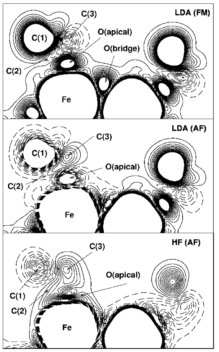
Figure 4: Rescaled plots of the spin densities for the ferromagnetic (FM) state at the LDA level (first graph) and for the antiferromagnetic (AF) state at the LDA (second graph) and the HF level (third graph).

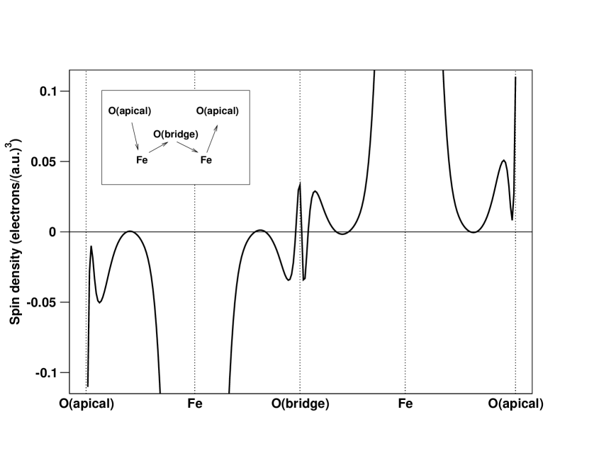
Figure 5: One-dimensional plot of the spin density at the LDA level for the antiferromagnetic state along a line between certain atoms of the molecule, see labeling of the abscissa and insert caption. The scaling of the ordinate refers to the values in table 4.

This feature is reflected in the spin-density plots in figure 3 and in larger resolution in figure 4. For a more detailed study, an one-dimensional plot of the spin-density at the LDA level along a line from O(apical) via Fe, O(bridge) and Fe to O(apical) was performed (figure 5). The iron atoms subsist in a high-spin state $3d^{5}_{\uparrow}\textit{d}^{0}_{\downarrow}$, but except for the HF method the moment is closer to $4\mu_{B}$ as it was also obtained by Postnikov et al for a slightly different moleculepostnikov2003 ; postnikov2004 . As can be seen in table 4, the local magnetic moment of the apical oxygen atoms increases from HF over B3LYP and PBE to LDA. In addition, there is a local magnetic moment at the carbon C(1) atom (see figure 1 and table 4) which is about 4 times (HF) to 2 times (LDA) smaller than the local magnetic moment of the apical oxygen atom. Corresponding to the moment of the C(1) atom there is a small magnetic moment at the carbon atoms C(2) and C(3), but with opposite sign and a much smaller value. Further on there is actually a moment at the first carbon atom (next to the carbon atoms C(2) and C(3)) of each $C_{6}H_{5}$ ring. Its value is of the same order as the value of the C(2) and C(3) carbon atoms moments, but with opposite sign. In the ferromagnetic state, there is a small magnetic moment at the C(4) bridge carbon atoms corresponding to the magnetic moment of the bridge oxygen atoms which is also, as already mentioned above, increasing from HF over B3LYP and PBE to LDA.

The results from the Mulliken population analysis of the iron, oxygen (bridge and apical), lithium and carbon atoms are given in tables 4 and 4. The net charge of iron is between 1.27 and 2.16, at the various levels of theory, and thus far away from a formal chargeAbbati1997 of +3. Again, Hartree-Fock gives a very localized picture with the largest net charge (2.16), and LDA a delocalized picture with an iron charge of only 1.27. Oxygen carries essentially a single negative charge ($\sim$ -0.8 in LDA, $\sim$ -1.1 in HF), the carbon atoms which have oxygen as a neighbor all have donated charge (0.4 - 0.8 $|e|$, depending on the site and the level of theory). The lithium charge is between 0.4 (LDA) and 0.8 (HF). A plot of the difference of the charge density was performed between the values at the LDA and HF level (figure 6). There is a positive charge density difference at the iron atoms because of the smaller charge at the LDA level compared to HF, the results for the other atoms follow from tables 4 and 4. This plot thus visualizes the more covalent picture obtained at the LDA level. The stronger covalency also becomes obvious in the Mulliken overlap population: for example, the overlap population between Fe and the neighbouring oxygens atoms is 0.11-0.12 at the LDA level, but only 0.07-0.08 at the HF level.

IV Summary

Ab-initio calculations for a hexanuclear ferric wheel Abbati1997 were performed. The exchange coupling parameter $J$ was computed at various levels of theory, with the B3LYP functional providing the best agreement with experiment (-31 K, experiment: -21 K). LDA and PBE were found to grossly overestimate the exchange coupling parameter due to the too large delocalization of the $d$-orbitals. Surprisingly, the calculation at the Hartree-Fock level led to a ferromagnetic coupling. The electronic population and the spin densities were calculated. The total spin is distributed over several sites, besides the iron atom all of the neighboring oxygens carry some spin. The delocalization increases from HF over B3LYP, PBE to LDA which shows the strongest delocalization and thus the smallest magnetic moment on the iron site.

V Acknowledgments

Most of the calculations were performed at the compute-server cfgauss (Compaq ES 45) of the data processing center of the TU Braunschweig. The geometry plot of the molecule was performed with MOLDENmolden .

Table 1: Total energies ($E_{h}\equiv$ Hartree), the differences in total energies for the ferromagnetic (FM) and the antiferromagnetic (AF) state and exchange parameters J

method	FM total energy $(E_{h})$	AF total energy $(E_{h})$	difference of total energy $(mE_{h})$	exchange parameter $J$ (K)
HF	-13295.7328681	-13295.7312480	-1.62	+7
HF (without Li)	-13287.8311111	-13287.8293232	-1.79	+8
B3LYP	-13334.5067552	-13334.5140876	7.33	-31
PBE	-13329.9510763	-13329.9768112	25.74	-108
LDA	-13273.9493819	-13273.9779682	28.58	-120

Table 2: Local magnetic moments at various sites, in $\mu_{B}$, for the ferromagnetic (FM) and the antiferromagnetic (AF) state

method	Fe		O (apical)		O (bridge)		C(1)		C(2)/C(3)		C(4)
	AF	FM	AF	FM	AF	FM	AF	FM	AF	FM	AF	FM
HF	$\pm 4.79$	$+4.79$	$\pm 0.04$	$+0.04$	$\approx 0$	$+0.07$	$\pm 0.008$	$+0.009$	$\mp 0.006$	$-0.006$	$\approx 0$	$\approx 0$
B3LYP	$\pm 4.32$	$+4.34$	$\pm 0.10$	$+0.10$	$\approx 0$	$+0.20$	$\pm 0.031$	$+0.032$	$\mp 0.007$	$-0.007$	$\approx 0$	+0.005
PBE	$\pm 4.10$	$+4.19$	$\pm 0.10$	$+0.11$	$\approx 0$	$+0.22$	$\pm 0.041$	$+0.046$	$\mp 0.005$	$-0.003$	$\approx 0$	+0.009
LDA	$\pm 3.96$	$+3.94$	$\pm 0.11$	$+0.11$	$\approx 0$	$+0.20$	$\pm 0.040$	$+0.047$	$\mp 0.003$	$-0.006$	$\approx 0$	+0.010

Table 3: Mulliken charge of Fe, in $|e|$. Note that the charge is virtually identical for the ferromagnetic and the antiferromagnetic state.

method	net charge	s	p	d
HF	2.16	6.28	12.28	5.29
B3LYP	1.56	6.38	12.37	5.69
PBE	1.40	6.39	12.37	5.84
LDA	1.27	6.43	12.41	5.89

Table 4: Charge at various sites, in $|e|$. Note that the charge is virtually identical for the ferromagnetic and the antiferromagnetic state.

method	Li	O (apical)	O (bridge)	C(1)	C(2)/C(3)	C(4)
HF	0.77	-1.10	-1.18	-0.22	0.82	0.50
B3LYP	0.53	-0.86	-0.88	-0.11	0.62	0.45
PBE	0.47	-0.79	-0.80	-0.10	0.56	0.38
LDA	0.38	-0.76	-0.75	-0.09	0.56	0.36

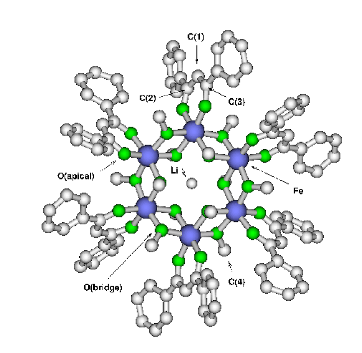
Figure 1: Geometry of the ferric wheel. Hydrogen atoms have been omitted for clarity.

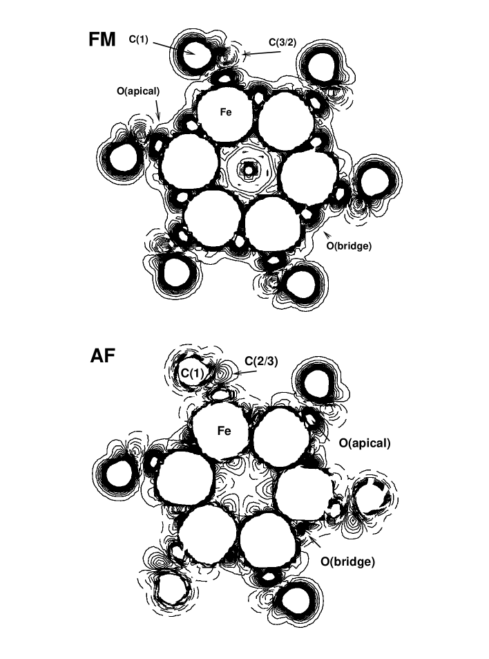
Figure 3: Spin densities at the LDA level for the ferromagnetic (FM) and the antiferromagnetic (AF) state. For all figures, the contour lines range from -0.0004 to 0.0005 in steps of 0.000035 electrons$/($a.u.$)^{3}$. Full lines indicate positive spin density and dashed lines indicate negative spin density.

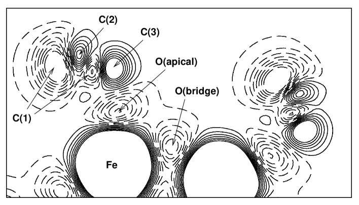
Figure 6: Rescaled plot of the charge density difference between the LDA and the HF level for the antiferromagnetic state. The contour lines range from -0.005 to 0.005 in steps of 0.0007 electrons$/($a.u.$)^{3}$. Full lines indicate positive charge density difference and dashed lines indicate negative charge density difference.

References

- (1) A. Caneschi, D. Gatteschi, C. Sangregorio, R. Sessoli, L. Sorace, A. Cornia, M. A. Novak, C. Paulsen and W. Wernsdorfer, J. Mag. Mag. Mat., 200 182 (1999)
- (2) B. Pilawa, Ann. Phys. (Leipzig), 8, 191 (1999)
- (3) A. V. Postnikov, J. Kortus and M .R. Pederson, newsletter, 61, 127 (February 2004)
- (4) M.D. Towler, N.L. Allan, N.M. Harrison, V.R. Saunders, W.C. Mackrodt and E. Aprà, Phys. Rev. B 50, 5041 (1994)
- (5) J. M. Ricart, R. Dovesi, C. Roetti and V. R. Saunders, Phys. Rev. B 52, 2381 (1995)
- (6) M. Catti, R. Valerio and R. Dovesi, Phys. Rev. B 51, 7441 (1995)
- (7) K. Fink, R. Fink and V. Staemmler, Inorg. Chem. 33, 6219 (1994)
- (8) K. Fink, C. Wang and V. Staemmler, Inorg. Chem. 38, 3847 (1999)
- (9) C. de Graaf, F. Illas, R. Broer and W. C. Nieuwpoort, J. Chem. Phys. 106, 3287 (1997)
- (10) M. Mödl, M. Dolg, P. Fulde and H. Stoll, J. Chem. Phys. 106, 1836 (1997)
- (11) E. Ruiz, M. Llunell and P. Alemany, J. Solid State Chem. 176, 400 (2003)
- (12) Z. Zeng, D. Guenzburger and D. E. Ellis, Phys. Rev. B 59, 6927 (1999)
- (13) I. de P. R. Moreira, F. Illas and R. L. Martin, Phys. Rev. B 65, 155102 (2002)
- (14) R. L. Martin and F. Illas, Phys. Rev. Lett. 79, 1539 (1997)
- (15) B. Normand, X. Wang, X. Zotos and D. Loss, Phys. Rev. B 63, 184409 (2001)
- (16) A. Honecker, F. Meier, D. Loss and B. Normand, Eur. Phys. J. B 27, 487 (2002)
- (17) A. Caneschi, A. Cornia and S. J. Lippard, Angew. Chem. 107, 511 (1995)
- (18) A. Caneschi, A. Cornia, A. C. Fabretti, S. Foner, D. Gatteschi, R. Grandi and L. Schenetti, Chem. Eur. J. 2, 1379 (1996)
- (19) G. L. Abbati, A. Cornia, A. C. Fabretti, W. Malavasi, L. Schenetti, A. Caneschi and D. Gatteschi, Inorg. Chem. 36, 6443 (1997).
- (20) A. Lascialfari, D. Gatteschi, F. Borsa and A. Cornia, Phys. Rev. B 55, 14341 (1997)
- (21) B. Pilawa, R. Desquiotz, M. T. Kelemen, M. Weickenmeier and A. Geisselmann, J. Mag. Mag. Mat. 177-181, 748 (1997)
- (22) R. W. Saalfrank, I. Bernt, E. Uller and F. Hampel, Angew. Chem. 109, 2596 (1997)
- (23) O. Waldmann, J. Schülein, R. Koch, P. Müller, I. Bernt, R. W. Saalfrank, H. P. Andres, H. U. Güdel and P. Allensbach, Inorg. Chem. 38, 5879 (1999)
- (24) M. Affronte, J. C: Jasjaunias, A. Cornia and A. Caneschi, Phys. Rev. B 60, 1161 (1999)
- (25) A. Cornia, A. G. M. Jansen and M. Affronte, Phys. Rev. B 60, 12177 (1999)
- (26) M. Affronte, A. Corina, A. Lascialfari, F. Borsa, D. Gatteschi, J. Hinderer, M. Horvatić, A. G. M. Jansen and M.-H. Julien, Phys. Rev. Lett. 88, 167201 (2002)
- (27) B. Pilawa, I. Keilhauer, G. Fischer, S. Knorr, J. Rahmer and A. Grupp, Eur. Phys. J. B 33, 321 (2003)
- (28) A. V. Postnikov, J. Kortus and S. Blügel, Mol. Phys. Rep. 38, 56 (2003)
- (29) A. V. Postnikov, S. G. Chiuzbăian, M. Neumann and S. Blügel, J. Phys. Chem. Solids 65, 813 (2004)
- (30) V. R. Saunders, R. Dovesi, C. Roetti, R. Orlando, C. M. Zicovich-Wilson, N. M. Harrison, K. Doll, B. Civalleri, I. J. Bush, P. D’Arco and M. Llunell, CRYSTAL2003 User’s Manual 2003
- (31) R. Dovesi, R. Orlando, C. Roetti, C. Pisani and V. R. Saunders, phys. stat. sol. (b) 217, 63 (2000)
- (32) J. P. Perdew and A. Zunger, Phys. Rev. B 23, 5048 (1981).
- (33) J. P. Perdew, K. Burke and M. Ernzerhof, Phys. Rev. Lett. 77, 3865 (1996).
- (34) Basis sets were obtained from the Extensible Computational Chemistry Environment Basis Set Database, Version 02/25/04, as developed and distributed by the Molecular Science Computing Facility, Environmental and Molecular Sciences Laboratory which is part of the Pacific Northwest Laboratory, P.O. Box 999, Richland, Washington 99352, USA, and funded by the U.S. Department of Energy. The Pacific Northwest Laboratory is a multi-program laboratory operated by Battelle Memorial Institute for the U.S. Department of Energy under contract DE-AC06-76RLO 1830. Contact David Feller or Karen Schuchardt for further information.
- (35) V. Rassolov, J. A. Pople, M. Ratner and T. L. Windus, J. Chem. Phys. 109, 1223 (1998).
- (36) R. Ditchfield, W. J. Hehre and J.A. Pople, J. Chem. Phys. 54, 724 (1971).
- (37) W. J. Hehre, R. Ditchfield and J. A. Pople, J. Chem. Phys. 56, 2257 (1972).
- (38) P. C. Hariharan and J. A. Pople, Theor. Chim. Acta 28, 213 (1973).
- (39) O. Waldmann, R. Koch, S. Schromm, J. Schülein, P. Müller, I. Bernt, R. W. Saalfrank, F. Hampel and E. Balthes, Inorg. Chem. 40, 2986 (2001)
- (40) O. Kahn, Molecular Magnetism, VCH Publishers Inc., New York (1993)
- (41) G. Schaftenaar and J. H. Noordik, J. Comput.-Aided Mol. Design, 14, 123 (2000)