Non-linear ripple dynamics on amorphous surfaces patterned by ion-beam sputtering

Abstract

Erosion by ion-beam sputtering (IBS) of amorphous targets at off-normal incidence frequently produces a (nanometric) rippled surface pattern, strongly resembling macroscopic ripples on aeolian sand dunes. Suitable generalization of continuum descriptions of the latter allows us to describe theoretically for the first time the main nonlinear features of ripple dynamics by IBS, namely, wavelength coarsening and non-uniform translation velocity, that agree with similar results in experiments and discrete models. These properties are seen to be the anisotropic counterparts of in-plane ordering and (interrupted) pattern coarsening in IBS experiments on rotating substrates and at normal incidence.

Ever since their earliest observation navez , the production of ripples on the surfaces of amorphous targets subject to ion-beam sputtering (IBS) at intermediate energies, has been fascinating due to the similarities with macroscopic ripples, like those produced underwater vortex_exp , or on the surface of aeolian sand dunes dunas . Beyond the morphological resemblance, IBS ripples share many other properties with e.g. aeolian ripples, such as wavelength coarsening and pattern translation with time carter ; habenicht . Remarkably, while typical wavelengths of the latter are above 1 cm, the periodicity of IBS ripples is in the 100 nm range valbusa , these patterns having gained increased interest recently for applications in Nanotechnology, ranging from optoelectronic to catalytic applic . IBS ripples are produced on a wide class of substrates, from amorphous or amorphizable (silica, Si, GaAs, InP) to metallic targets (Cu, Au, Ag) valbusa . In view moreover of their implied loss of in-plane symmetry, IBS ripples provide interesting instances of systems hosting a competition between pattern forming and disordering mechanisms patt .

A successful description of the main features of IBS ripples was provided by Bradley and Harper (BH) BH , based on Sigmund’s linear cascade approximation of sputtering processes in amorphous or polycrystalline targets Sigmund . The linear equation derived by BH describes satisfactorily some properties of IBS ripples, such as their alignment with the ion beam as a function of the incidence angle to target normal $\theta$ [wave vector parallel (perpendicular) to the projection of the ion beam for $\theta<\theta_{c}$ ($\theta>\theta_{c}$), for some threshold $\theta_{c}$]. Other features, such as ripple stabilization or wavelength dependence with ion energy or flux, required non-linear extensions of BH’s approach Makeev ; park , leading to an anisotropic generalization of the well known Kuramoto-Sivashinsky (KS) equation patt ; Makeev . However, a notable limitation of the anisotropic KS (AKS) equation is its inability to predict ripples that coarsen with time, contradicting observations in many experiments and/or discrete models of IBS (see habenicht ; yewande and Refs. therein).

In this Letter, we introduce a “hydrodynamic” model dunas ; Aste ; prl for IBS ripple production at off-normal incidence. Time scale separation between microscopic processes (collision cascades, surface diffusion) and pattern evolution allows us to derive an improved equation for the surface height. The new non-linear terms appearing allow for ripple coarsening and pattern translation with non-uniform velocity, as seen in experiments and discrete models. Our theory has both the AKS equation Makeev and the normal incidence hydrodynamic theory prl ; normal as particular limits, and enables analysis of the important case of rotating substrates frost . In addition, our model may be important also to the context of ripples on aeolian sand dunes, where the standard 1D approximation requires validation, fully anisotropic 2D models being scarce dunas , as incidentally occurs in many other contexts within Pattern Formation bar_nepomnyaschy2 .

During IBS of amorphous or semiconductor substrates, in which the ions amorphize the subsurface layer, incident ions lose their energy through random collision cascades in the bulk Sigmund . Near-surface atoms receiving enough energy and momentum to break their bonds are in principle sputtered away, although they may join the current of surface adatoms that are available to other relaxation mechanisms, such as surface diffusion, before incorporating back to the solid bulk. Within the so-called “hydrodynamic” approach to aeolian sand dunes dunas and ion-sputtered surfaces Aste ; prl , we consider two coupled fields, namely, the thickness of the mobile surface adatoms layer, $R(\mathbf{x},t)$, (related with the density of mobile adatoms through the atomic volume) and the height of the bombarded surface above a reference plane, $h(\mathbf{x},t)$. Their time evolution is provided by

$$\partial_{t}R =(1-\phi)\Gamma_{ex}-\Gamma_{ad}+D\nabla^{2}R,$$ (1)

$$\partial_{t}h =-\Gamma_{ex}+\Gamma_{ad},$$ (2)

where $\Gamma_{ex}$ and $\Gamma_{ad}$ are, respectively, rates of atom excavation from and addition to the immobile bulk, $(1-\phi)=\bar{\phi}$ measures the fraction of eroded atoms that become mobile, and the third term in Eq. (1) describes motion of mobile atoms along the surface as due to isotropic thermal diffusion ($D$ being a constant for amorphous materials). Even if all eroded atoms are sputtered away ($\phi=1$), we assume a non-zero average fraction of mobile atoms, $R_{eq}$.

Under the assumption that nucleation events are more likely in surface protrusions, in analogy to the Gibbs-Thompson relation we have

$$\Gamma_{ad}=\gamma_{0}\left[R(1+\gamma_{2x}\partial^{2}_{x}h+\gamma_{2y}\partial^{2}_{y}h)-R_{eq}\right],$$ (3)

where $\gamma_{0}$ is the mean nucleation rate for a flat surface (on the $xy$ plane) and $\gamma_{2x}$, $\gamma_{2y}\geq 0$ describe variation of the nucleation rate with surface curvatures. Note that, in (3), the full thickness of the mobile adatoms layer is affected by the shape of the surface.

The rate at which material is sputtered from the bulk depends on the angle of incidence, ion and substrate species, ion flux, energy, and many other experimental parameters. If the beam direction is in the $xz$ plane, we have, following Makeev ; prl

$$\Gamma_{ex}=\alpha_{0}\big{[}1+\alpha_{1x}\partial_{x}h+\alpha_{2x}\partial^{2}_{x}h+\alpha_{2y}\partial^{2}_{y}h\\ +\alpha_{3x}(\partial_{x}h)^{2}+\alpha_{3y}(\partial_{y}h)^{2}-(\partial_{x}h)(\alpha_{4x}\partial^{2}_{x}h+\alpha_{4y}\partial^{2}_{y}h)\big{]},$$ (4)

where parameters reflect the dependence of $\Gamma_{ex}$ on the local shape of the surface detalles , as described by more microscopic derivations such as BH or generalizations thereof Makeev ; Feix . Analogous, but not equal, geometrical couplings to the driving occur in aeolian sand dunes dunas , or in growth onto amorphous substrates Raible . Note the loss of reflection symmetry in the $x$ direction, but not in the $y$ direction. For a planar surface, atoms are sputtered from the bulk in a typical time of order $\alpha_{0}^{-1}$.

The main difference between former models BH ; Makeev ; park and our present model, Eqs. (1)-(4), is that, in the latter, eroded material is allowed to redeposit locally, and there is an implicit viscous flow viscousflow in the amorphized layer through the evolution of $R$. These additional mechanisms are seen below to induce richer pattern dynamics than in BH ; Makeev ; park .

The linearized Eqs. (1)-(4) have solutions ${R}^{l}=\hat{R^{l}}e^{i\mathbf{k\cdot x}+\omega_{\mathbf{k}}t}$, $h^{l}=\hat{h^{l}}e^{i\mathbf{k\cdot x}+\omega_{\mathbf{k}}t}$, with a dispersion relation, $\omega_{\mathbf{k}}$, given in the long wavelength limit by detalles

$$\ \mathcal{R}e(\omega_{\mathbf{k}}) = \epsilon\phi\gamma_{0}(\alpha_{2x}k_{x}^{2}+\alpha_{2y}k_{y}^{2})-\epsilon^{2}\phi\bar{\phi}\gamma_{0}\alpha_{1x}^{2}k_{x}^{2}$$

$$-R_{eq}D(k_{x}^{2}+k_{y}^{2})(\gamma_{2x}k_{x}^{2}+\gamma_{2y}k_{y}^{2})+\mathcal{O}(\epsilon k^{4}),$$ (5)

$$\mathcal{I}m(\omega_{\mathbf{k}}) = -\epsilon\phi\gamma_{0}\alpha_{1x}k_{x}+\mathcal{O}(k^{3}),$$ (6)

where $\epsilon\equiv\alpha_{0}/\gamma_{0}$ is a dimensionless parameter; the erosion rate being much smaller than the nucleation rate, $\epsilon\ll 1$ for typical experiments. Eq. (6) is a simple consequence of the asymmetry in the $x$ direction, induced by the incoming flux.

The surface morphology is dominated by the periodic pattern with wave vector $\mathbf{k}^{max}$ making Eq. (5) a positive maximum. It can be shown detalles that $\mathbf{k}^{max}$ is oriented along the $\mathbf{\hat{x}}$ or $\mathbf{\hat{y}}$ directions, as observed experimentally valbusa . Close to the instability threshold, before nonlinear terms are no longer negligible, one has $k_{x,y}^{max}\sim\epsilon^{1/2}$. Substituting this into Eqs. (5) and (6) provides us with estimations of the typical time and length scales of the pattern, that we employ to rescale $X=\epsilon^{1/2}x$, $Y=\epsilon^{1/2}y$, $T_{2}=\epsilon^{2}t$ and $T_{1}=\epsilon^{3/2}t$, and perform a multiple scale expansion of Eqs. (1), (2), in which $R$ can be adiabatically eliminated. To lowest non-linear order, we get detalles ; nota_no_redep

$$\partial_{t}h =\gamma\partial_{x}h+\sum_{i=x,y}\Bigl{\{}-\nu_{i}\,\partial^{2}_{i}h+\lambda^{(1)}_{i}\,(\partial_{i}h)^{2}+\Omega_{i}\partial_{i}^{2}\partial_{x}h$$

$$+\xi_{i} (\partial_{x}h)(\partial^{2}_{i}h)\Bigr{\}}+\sum_{i,j=x,y}\Bigl{\{}-{\cal K}_{ij}\partial^{2}_{i}\partial^{2}_{j}h+\lambda^{(2)}_{ij}\partial^{2}_{i}(\partial_{j}h)^{2}\Bigr{\}};$$

$$\gamma =-\epsilon\phi\gamma_{0}\alpha_{1x},\quad\nu_{x}=\epsilon\phi\gamma_{0}\alpha_{2x}-\epsilon^{2}\bar{\phi}\phi\gamma_{0}\alpha_{1x}^{2},$$

$$\nu_{y} =\epsilon\phi\gamma_{0}\alpha_{2y},\quad\lambda_{i}^{(1)}=-\epsilon\phi\gamma_{0}\alpha_{3i},$$

$$\Omega_{i} =\epsilon(\bar{\phi}D-\phi R_{eq}\gamma_{0}\gamma_{2i})\alpha_{1x},\quad\xi_{i}=\epsilon\phi\gamma_{0}\alpha_{4i},$$

$${\cal K}_{ij} =DR_{eq}\gamma_{2i}+\epsilon\big{[}D\bar{\phi}(\gamma_{2i}-\alpha_{2j})+\phi\gamma_{0}R_{eq}\gamma_{2i}\alpha_{2j}\big{]},$$

$$\lambda^{(2)}_{ij} =\epsilon\big{[}\bar{\phi}D-\phi R_{eq}\gamma_{0}\gamma_{2i}\big{]}\alpha_{3j}.$$ (7)

Eq. (7) generalizes the AKS type equations obtained BH ; Makeev ; park within BH approach to IBS. While sharing the same reflection properties in the $x$ and $y$ directions and most of the terms on the rhs, both equations differ crucially by the presence here of the $\lambda^{(2)}_{ij}$ nonlinearities. Moreover, in the absence of redeposition ($\phi=1$), $\lambda^{(1)}_{i}$ and $\lambda^{(2)}_{ij}$ have the same signs, making Eq. (7) nonlinearly unstable, as in the BH case prl ; Kim ; comments . Note, the linear dispersion relation of (7) matches Eqs. (5) and (6) above. Under normal incidence, parameters are isotropic and $\alpha_{1x}=\alpha_{4x}=\alpha_{4y}=0$, Eq. (7) reducing to that obtained in prl ; Kim , and in Raible . As a final remark, let us quote the form of Eq. (7) for sample rotation around the $z$ axis during bombardment (see e.g. Bradley ; frost ). Dynamics of $h$ are given by a different isotropic limit of Eq. (7), namely,

$$\partial_{t}h =-\nu_{\rm r}\nabla^{2}h-{\cal K}_{\rm r}\nabla^{4}h+\lambda^{(1)}_{\rm r}(\nabla h)^{2}+\lambda^{(2)}_{\rm r}\nabla^{2}(\nabla h)^{2}$$

$$+\lambda^{(3)}_{\rm r}\,\nabla\cdot\big{[}(\nabla^{2}h)\nabla h\big{]}\big{]};$$ (8)

$$\nu_{\rm r} =(\nu_{x}+\nu_{y})/2,\quad\lambda^{(1)}_{\rm r}=(\lambda^{(1)}_{x}+\lambda^{(1)}_{y})/2,$$

$$\lambda^{(2)}_{\rm r} =\frac{1}{4}\sum_{i,j=x,y}\lambda^{(2)}_{i,j},\quad\lambda^{(3)}_{\rm r}=\frac{1}{2}\sum_{i,j=x,y}\lambda^{(2)}_{i,j}\delta_{i,j}-\lambda^{(2)}_{\rm r},$$

$$\cal K_{\rm r} =(3{\cal K}_{x,x}+3{\cal K}_{y,y}+{\cal K}_{x,y}+{\cal K}_{y,x})/8,$$

with parameters (susbscript “r” denotes “rotating”).

To the best of our knowledge, Eq. (7) is new, and indeed has a rich parameter space. Numerical integration (not shown) within linear regime retrieves all features of the ripple structure as predicted by the BH theory, i.e., dependence of the ripple wavelength with linear terms, and ripple orientation as a function of $\theta$. Entering the nonlinear regime, and as occurs in the AKS equation and its generalizations Makeev ; park , nonlinearities $\lambda^{(1)}_{i}$ lead to saturation of the pattern with constant wavelength and amplitude. In absence of these terms, the ripple wavelength grows indefinitely as $\ell(t)\sim t^{n}$ with $n=1/2$ Raible_b ; nota_exponente until a single ripple remains in a finite simulation domain. As an anisotropic generalization of the ordering process observed for normal incidence prl ; normal , pattern coarsening requires the presence of $\lambda^{(2)}_{i,j}$, whose magnitude and mathematically correct sign comments are due to describing redeposition by means of the additional field $R$. When the values of these coefficients increase relative to $\lambda^{(1)}_{i}$, coarsening stops later, and the amplitude and wavelength of the pattern also increase. The coarsening exponent $n$ will take an effective value that will be larger the later coarsening stops, and may depend on simulation parameter values. For instance, we show in Fig. 1 snapshots of a numerical integration of Eq. (7) for relatively large $\lambda^{(2)}_{i,j}$. The apparent coarsening is quantified in the plot of $\ell(t)$ shown in Fig. 2$(a)$, compatible (after transient effects analogous to those in Raible_b ) with $n=0.19$. Note the saturation of ripple wavelength at long times, together with saturation in amplitude, as shown in the plot of the surface roughness (rms width) $W(t)$ in Fig. 2$(b)$. These results are similar to those obtained experimentally for IBS of Si in carter . For a different experiment on Si, precise measurements of the coarsening exponent habenicht yield $n=0.50(4)$, no saturation having been observed in this system, as we would expect. Here, the dispersion velocity of the pattern was also measured, finding that it decays with ripple wavelength or, equivalently, with time. We have also observed the same trend in the dispersion velocity of the ripples shown in Fig. 1. Experiments also exist, e.g. for IBS of Si, in which ripple coarsening is absent or residual erlebacher , that would correspond to smaller $\lambda^{(2)}_{i,j}$ values in (7), see e.g. an example in Fig. 3, where $\ell(t)\sim\log t$ approximately. Ripple coarsening has been also observed in a Monte Carlo model of IBS yewande , in which rules implement Sigmund’s theory. To our purpose, the main conclusion of this study is the correlation between an increasing $\ell(t)$ and non-uniform dispersion velocity, and on the parameter-dependent values of the coarsening exponent. Let us note that, on the experimental side, values of $n$ show a large scatter in the literature (see Refs. in valbusa ; yewande ).

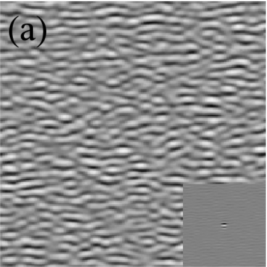
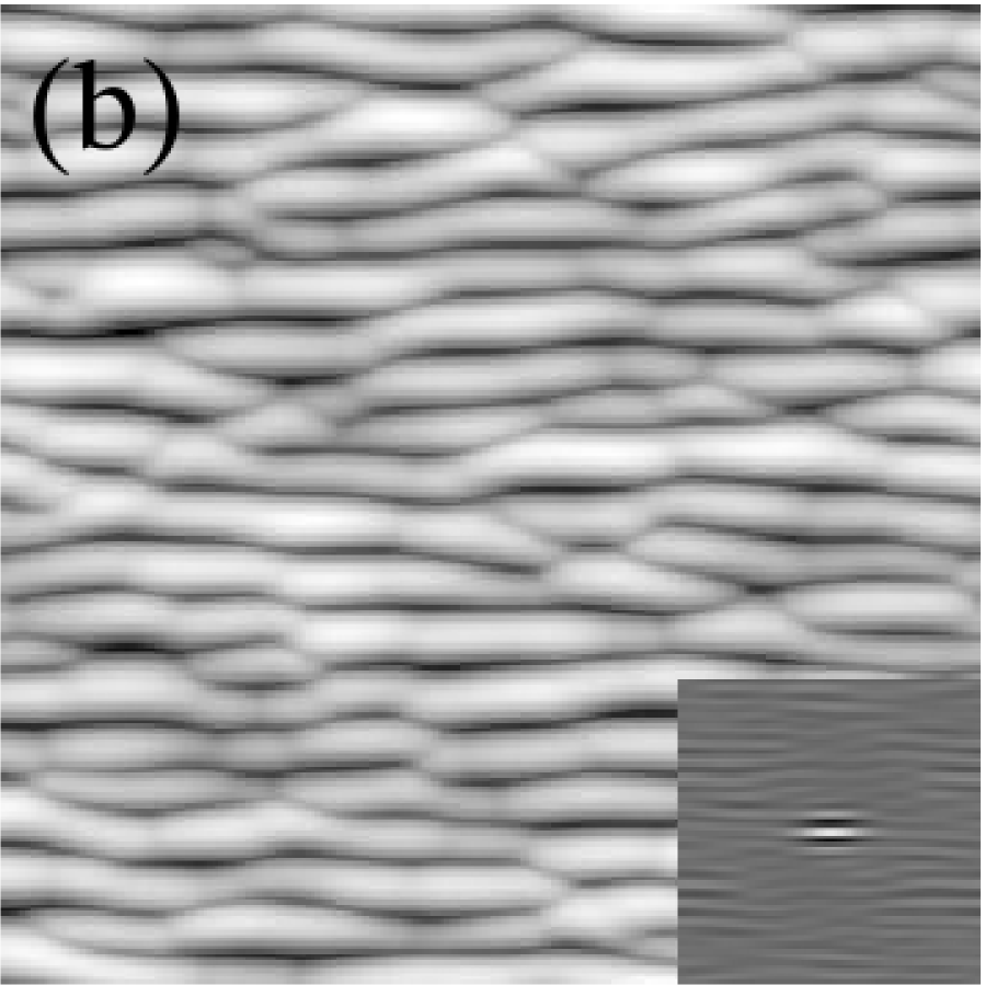
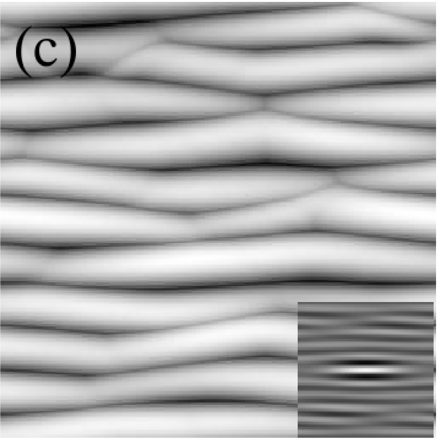
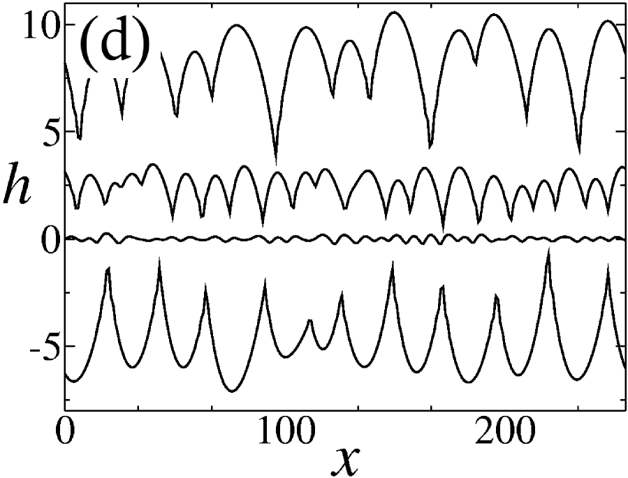
Figure 1: Numerical integration of Eq. (7) using $\nu_{x}=1$, $\nu_{y}=0.1$, $\Omega_{x}=1$, $\Omega_{y}=0.5$, $\xi_{i}=0.1$, $\lambda_{x}^{(1)}=0.1$, $\lambda_{y}^{(1)}=5$, $\lambda^{(2)}_{i,j}=-5$, ${\cal K}_{i,j}=1$. Top views for $t=10,106,953$ $(a)$, $(b)$, and $(c)$, respectively. Insets are height autocorrelations. All units are arbitrary. $(d)$: Top to bottom, side cuts of $(c)$, $(b)$, $(a)$, and grooves obtained for sign-changed $\lambda^{(1)}_{x,y}$ and $\lambda^{(2)}_{i,j}$. Curves have an artificial offset.

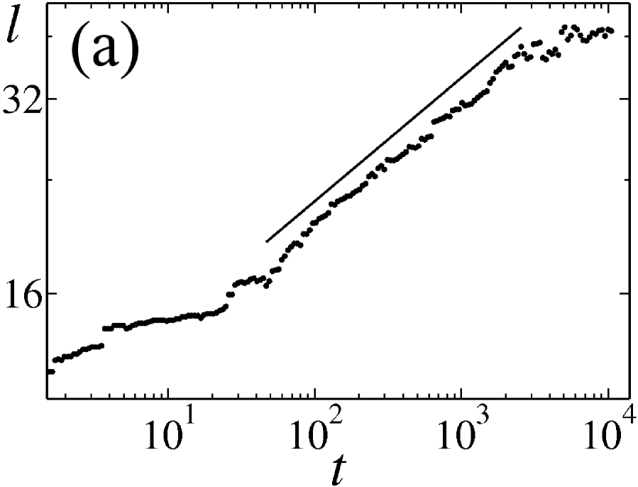
Figure 2: Ripple wavelength $\ell(t)$ and surface roughness $W(t)$ for parameters as in Fig. 1. The straight line represents $\ell\sim t^{0.19}$. All units are arbitrary.

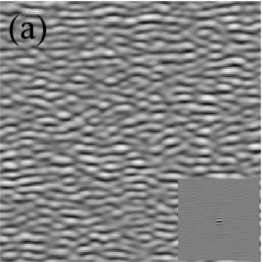
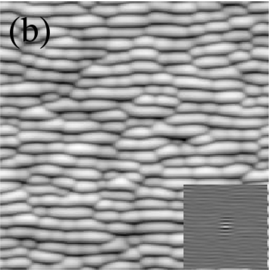
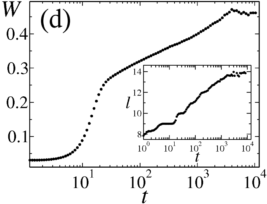
Figure 3: Numerical integration of Eq. (7) for parameters as in Fig. 1, except for $\lambda_{x}^{(1)}=1$. Top views for $t=10,106,953$ $(a)$, $(b)$, and $(c)$, respectively. $(d)$: Surface roughness $W(t)$ for the same simulation. Inset: $\ell(t)$ for the same system, showing marginal coarsening. All units are arbitrary.

Additional non-linear effects can be described by Eq. (7). A first one is production of grooves (as opposed to ripples), due to the loss of up-down symmetry induced by quadratic nonlinearities. Indeed, by changing the sign of $\lambda_{i}^{(1)}$, grooves replace ripples, see Fig. 1$(d)$; this calls for systematic experimental exploration. A second effect is related with cancellation modes (CM), known in the AKS equation rost_krug ; park and other models of IBS Aste ; prl ; Kim . These are linearly unstable modes for which nonlinearities cancel one another exactly. While for equations like the one considered in prl ; Raible CM affect well-posedness, anisotropic systems rost_krug ; park may remain better defined in the presence of CM. In our case, if reflection symmetry breaking terms are neglected in Eq. (7) and BH parameters are used, the same CM occur as in the AKS equation. Additional CM ensue between the $\lambda_{i}^{(1)}$ and $\lambda^{(2)}_{i,j}$ terms for appropriate relative signs Raible ; comments . We have verified numerically that the full Eq. (7) breaks down for the latter CM, but can support AKS-type CM. That these solutions are physically realizable or are artifacts of the small slope approximation made, remains to be assessed. Useful information on this issue might come from field experiments in aeolian sand dunes.

In closing, we mention IBS of metals as an immediate experimental domain to which the above results may be relevant valbusa , albeit differing in the degree of universality. There, however, the correct extension of BH theory is not yet clear, nor is its importance relative to anisotropic surface diffusion. We have taken preliminar steps in this context Feix , and expect to make progress in this direction soon.

- (1) M. Navez, C. Sella, and D. Chaperot, C. R. Acad. Sci. Paris 254, 240 (1962).
- (2) A. Stegner and J. E. Wesfreid, Phys. Rev. E 60, R3487 (1999).
- (3) O. Terzidis, P. Claudin and J.-P. Bouchaud, Eur. Phys. J. B 5, 245 (1998); A. Valance and F. Rioual, Eur. Phys. J. B 10, 543 (1999); Z. Csahók et al., Eur. Phys. J. E 3, 71 (2000).
- (4) G. Carter and V. Vishnyakov, Phys. Rev. B 54, 17647 (1996).
- (5) S. Habenicht et al., A. D. Wieck, Phys. Rev. B 65, 115327 (2002).
- (6) U. Valbusa, C. Boragno, and F. Buatier de Mongeot, J. Phys. Condens. Matter 14, 8153 (2002).
- (7) M. V. R. Murty, Surf. Sci. 500, 523 (2002); O. Azzaroni et al., Adv. Mater. 16, 405 (2004).
- (8) M. C. Cross and P. C. Hohenberg, Rev. Mod. Phys. 65, 851 (1993).
- (9) R. M. Bradley and J. M. Harper, J. Vac. Sci. Technol. A 6, 2390 (1988).
- (10) P. Sigmund, Phys. Rev. 184, 383 (1969); J. Mat. Sci. 8, 1545 (1973).
- (11) R. Cuerno and A.-L. Barabási, Phys. Rev. Lett. 74, 4746 (1995); M. Makeev, R. Cuerno, and A.-L. Barábasi, Nucl. Instrum. Methods Phys. Res., Sect. B 197, 185 (2002).
- (12) S. Park et al. Phys. Rev. Lett. 83, 3486 (1999).
- (13) E. Yewande, A. K. Hartmann, and R. Kree, Phys. Rev. B 71, 195405 (2005).
- (14) T. Aste and U. Valbusa, Physica A 332, 548 (2004); New J. Phys. 7, 122 (2005).
- (15) M. Castro et al., Phys. Rev. Lett. 94, 016102 (2005).
- (16) S. Facsko et al., Science 285, 1551 (1999); R. Gago et al., Appl. Phys. Lett. 78, 3316 (2001).
- (17) F. Frost, A. Schindler, and F. Bigl, Phys. Rev. Lett. 85, 4116 (2000).
- (18) D. E. Bar and A. A. Nepomnyashchy, Physica D 132, 411 (1999).
- (19) J. Muñoz-García, M. Castro, and R. Cuerno, in preparation.
- (20) M. Feix et al., Phys. Rev. B 71, 125407 (2005).
- (21) M. Raible et al., Europhys. Lett. 50, 61 (2000); M. Raible, S. J. Linz, and P. Hänggi, Phys. Rev. E 64, 031506 (2001).
- (22) C. C. Umbach et al., Phys. Rev. Lett. 87, 246104 (2001).
- (23) In principle, Eq. (7) does not cover the conserved limit (irrelevant to IBS), where a different expansion must be used, as seen from Eqs. (5), (6).
- (24) T. C. Kim et al., Phys. Rev. Lett. 92, 246104 (2004).
- (25) M. Castro and R. Cuerno, Phys. Rev. Lett. 94, 139601 (2005); T. C. Kim et al., ibid. 94, 139602 (2005).
- (26) R. M. Bradley, Phys. Rev. E 54, 6149 (1996).
- (27) M. Raible, S. J. Linz, and P. Hänggi, Phys. Rev. E 62, 1691 (2000).
- (28) This is in absence of advective terms. Otherwise, even larger exponent values are possible detalles .
- (29) J. Erlebacher et al., Phys. Rev. Lett. 82, 2330 (1999).
- (30) M. Rost and J. Krug, Phys. Rev. Lett. 75, 3894 (1995).