The non-classical scissors mode of a vortex lattice in a Bose-Einstein condensate

Abstract

We show that a Bose-Einstein condensate with a vortex lattice in a rotating anisotropic harmonic potential exhibits a very low frequency scissors mode. The appearance of this mode is due to the SO(2) symmetry-breaking introduced by the vortex lattice and, as a consequence of this, its frequency tends to zero with the trap anisotropy $\epsilon$, with a generic $\sqrt{\epsilon}$ dependence. We present analytical formulas giving the mode frequency in the low $\epsilon$ limit and we show that the mode frequency for some class of vortex lattices can tend to zero as $\epsilon$ or faster. We demonstrate that the standard classical hydrodynamics approach fails to reproduce this low frequency mode, because it does not contain the discrete structure of the vortex lattice.

Since their first observations in 1995 Cornell95 ; Ketterle95 , the trapped gaseous atomic Bose-Einstein condensates have been the subject of intense experimental revue_experiments and theoretical revue_theory investigation. A fruitful line of studies has been the measurement of the eigenmode frequencies of the Bose-Einstein condensate, which can be performed with a very high precision and therefore constitutes a stringent test of the theory. Of particular interest in the context of superfluidity are the scissors modes, first introduced in nuclear physics nuclear and occurring in quantum gases stored in a weakly anisotropic harmonic trap. These scissors modes have been studied theoretically Odelin and observed experimentally Foot in a non-rotating gas, both in a condensate (where they have a large frequency even in the limit of a vanishing trap asymmetry) and in a classical gas (where their frequency tends to zero in a vanishing trap asymmetry limit).

Another fruitful line of studies has been the investigation of rotating Bose-Einstein condensates: above a critical rotation frequency of the anisotropic trap, it was observed experimentally that vortices enter the condensate and settle into a regular lattice Dalibard ; Ketterle ; Cornell . In this paper, we study theoretically the scissors modes of a Bose-Einstein condensate with several vortices present, a study motivated by the discovery of a low frequency scissors mode in three-dimensional simulations in crystal . In section I, we define the model and the proposed experiment, and we present results from a numerical integration of the Gross-Pitaevskii equation: condensates with several vortices present have a scissors mode with a very low frequency, unlike non-rotating condensates. We show in section II that the equations of classical hydrodynamics, often used to describe condensates with a very large number of vortices hydro_class , fail to reproduce our numerical experiment. Then, in the central part of our paper, section III, we interpret this mode in terms of a rotational symmetry breaking due to the presence of the vortices, which gives rise for $\epsilon=0$ to a Goldstone mode of zero energy, becoming for finite $\epsilon$ a low frequency scissors mode and this leads to an explanation for the failure of the classical hydrodynamics approximation. We then use Bogoliubov theory in section IV to obtain an upper bound on the frequency on the scissors mode, which reveals that two situations may occur: in what we call the non-degenerate case, the frequency of the scissors mode tends to zero as the square root of the trap anisotropy, and we show with perturbation theory that the upper bound gives the exact result in this limit. In the opposite degenerate case, the frequency of the scissors mode tends to zero at least linearly in the trap anisotropy, and this we illustrate with a numerical calculation of the mode frequency for a three-vortex configuration. We conclude in section V.

I Model and a numerical simulation

We consider a weakly interacting quasi two-dimensional (2D) Bose-Einstein condensate in an anisotropic harmonic trap rotating at the angular frequency $\Omega$ quasi2D . In the rotating frame, the trapping potential is static and given by

$$U(x,y)=\frac{1}{2}m\omega^{2}\left[(1-\epsilon)x^{2}+(1+\epsilon)y^{2}\right]$$ (1)

where $m$ is the mass of an atom, $\epsilon>0$ is the trap anisotropy and $\omega$ is the mean oscillation frequency of the atoms. From now on, we shall always remain in the rotating frame.

The condensate is initially in a stationary state of the Gross-Pitaevskii equation:

$$\left[-\frac{\hbar^{2}}{2m}\Delta+g|\psi|^{2}+U-\Omega L_{z}-\mu\right]\psi=0$$ (2)

where $g$ is the 2D coupling constant describing the atomic interactions Dum , $\mu$ is the chemical potential, $\psi$ is the condensate field normalized to the number of particles $N$ and $L_{z}=xp_{y}-yp_{x}$ is the angular momentum operator along $z$. In this paper, we shall concentrate on the case that the rotation frequency $\Omega$ is large enough so that several vortices are present in the field $\psi$, forming a regular array.

The standard procedure to excite the scissors mode is to rotate abruptly the trapping potential by a small angle $\theta$ and to keep it stationary afterwards. This is theoretically equivalent to abruptly rotating the field $\psi$ by the angle $-\theta$ while keeping the trap unperturbed:

$$\psi(t=0^{+})=e^{i\theta L_{z}/\hbar}\psi(t=0^{-}).$$ (3)

The subsequent evolution of $\psi$ is given by the time dependent Gross-Pitaevskii equation.

We have solved this time dependent Gross-Pitaevskii equation numerically, with the FFT splitting techniques detailed in Dum , the initial state being obtained by the conjugate gradient method Modugno . The results for a 4-vortex and a 10-vortex configurations are shown in figure 1 for $\epsilon=0.025$, for an initial rotation of the trapping potential by an angle of 10 degrees: we see a small amplitude slow oscillation of the vortex lattice as a whole around the new axis of the trap, accompanied by weak internal oscillations of the lattice and of the condensate. This suggests that, in this low $\epsilon$ limit, the excitation procedure mainly excites the scissors mode, and that this scissors mode has a very low frequency, much lower than the trap frequency $\omega$.

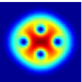
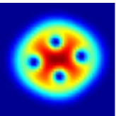
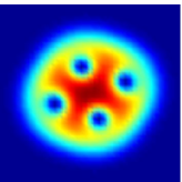
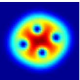
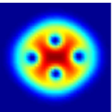
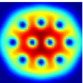
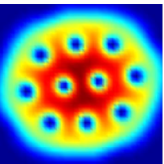
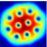
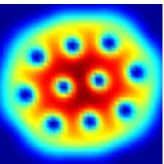
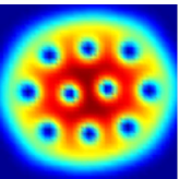
Figure 1: For an initial stationary condensate with vortices, numerical simulation of the excitation procedure of the scissors mode, by rotation of the trap by 10 degrees: density maps at successive times. Top row: 4-vortex configuration, with $N=2500$ atoms and a trap rotation frequency $\Omega=0.7\omega$, resulting in $\mu\simeq 4.6\hbar\omega$; the oscillation period is $\sim 265\omega^{-1}$ and the frames are separated by one quarter of a period. Bottom row: 10-vortex configuration, with $N=6000$ atoms and a trap rotation frequency $\Omega=0.8\omega$, resulting in $\mu\simeq 5.9\hbar\omega$; the oscillation period is $\sim 245\omega^{-1}$ and the frames are separated by one quarter of a period. The trap anisotropy is $\epsilon=0.025$, the coupling constant is $g=0.0343\hbar^{2}/m$. We have watched these oscillations without seeing significant damping over 7 periods.

II Classical hydrodynamics

In the approximation of a coarse-grained vorticity, a condensate with many vortices is described by a density profile $\rho(\mathbf{r})$ and a velocity field $\mathbf{v}(\mathbf{r})$ solving the classical hydrodynamics equations:

$$\left(\partial_{t}+\mathbf{v}\cdot\mathbf{grad}\right)\mathbf{v} = -\frac{1}{m}\mathbf{grad}\,(U+\rho g)-2\mathbf{\Omega}\times\mathbf{v}-\mathbf{\Omega}\times(\mathbf{\Omega}\times\mathbf{r})$$ (4)

$$\partial_{t}\rho+\mathrm{div}\,\rho\mathbf{v} = 0.$$ (5)

The first equation is Euler’s equation in the rotating frame, including the Coriolis and centrifugal forces. The second one is the continuity equation.

The velocity field $\mathbf{v}$ is the velocity field of the fluid in the rotating frame. In a stationary state, we set $\mathbf{v}=\mathbf{0}$ which amounts to assuming the solid body velocity field $\mathbf{\Omega}\times\mathbf{r}$ in the lab frame. The corresponding stationary density profile is given by a quadratic ansatz:

$$\rho_{0}(x,y)=\frac{m}{g}(\mu-a_{1}x^{2}-a_{2}y^{2}).$$ (6)

From Eq.(4) one then finds

$$a_{1,2}=\frac{1}{2}\left[\omega^{2}(1\mp\epsilon)-\Omega^{2}\right].$$ (7)

What happens after the rotation of the density profile by a small angle? To answer this question analytically, we linearize the hydrodynamics equations around the steady state, setting $\rho=\rho_{0}+\delta\rho$ and $\mathbf{v}=\delta\mathbf{v}$:

$$\partial_{t}\delta\mathbf{v} = -\frac{1}{m}\mathbf{grad}\,\delta\rho g-2\mathbf{\Omega}\times\delta\mathbf{v}$$ (8)

$$\partial_{t}\delta\rho+\mathrm{div}\,\rho_{0}\delta\mathbf{v} = 0.$$ (9)

At time $t=0^{+}$, $\delta\mathbf{v}=0$ and, to first order in the rotation angle $\theta$, $\delta\rho=2\theta mxy(a_{1}-a_{2})/g$. The subsequent evolution is given by the time dependent polynomial ansatz:

$$\delta\rho = \frac{m}{g}\left[c(t)-\mathbf{r}\cdot\delta A(t)\mathbf{r}\right]$$ (10)

$$\delta\mathbf{v} = \delta B(t)\mathbf{r}$$ (11)

where $\delta A(t)$ is a time-dependent 2$\times$2 symmetric matrix and $\delta B(t)$ is a time-dependent 2$\times$2 general matrix. These matrices evolve according to

$$\delta\dot{A} = -A\mathrm{Tr}\delta B(t)-A\delta B(t)-\delta B^{T}(t)A$$ (12)

$$\delta\dot{B} = 2\,\delta A(t)+2\Omega\begin{pmatrix}0&1\\ -1&0\end{pmatrix}\delta B(t)$$ (13)

where we have set $A=\begin{pmatrix}a_{1}&0\\ 0&a_{2}\end{pmatrix}$. The constant term evolves as $\dot{c}+\mu{\rm Tr}\delta B=0$.

First, one may look for eigenfrequencies of the system solved by $\delta A$ and $\delta B$. For $\epsilon=0$, this may be done analytically Cozzini : one finds one mode of zero frequency, and 6 modes of non-zero frequencies:

$$\nu=\pm 2\omega,\pm\left[(2\omega^{2}-\Omega^{2})^{1/2}+\Omega\right],\pm\left[(2\omega^{2}-\Omega^{2})^{1/2}-\Omega\right].$$ (14)

At this stage, the presence of a zero energy mode for vanishing anisotropy looks promising to explain the low frequency of the scissors mode. At weak but non-zero $\epsilon$, however, a numerical diagonalization of the resulting 7$\times$7 matrix shows that the zero frequency is unchanged, whereas the others change very little. Analytically, one then easily finds the zero-frequency mode for arbitrary $\epsilon$:

$$\delta A=-\Omega A\ \ \ \ \ \ \delta B=\begin{pmatrix}0&-a_{2}\\ a_{1}&0\end{pmatrix}$$ (15)

Why is there such a zero-frequency mode in the classical hydrodynamics? We have found that this is because there a continuous branch of stationary solutions of the classical hydrodynamics equations parametrized by two real numbers $\alpha$ and $\beta$:

$$\mathbf{v} = \begin{pmatrix}\alpha y\\ \beta x\end{pmatrix}$$ (16)

$$g\rho/m = \mu-a_{+}x^{2}-a_{-}y^{2}$$ (17)

where

$$a_{+} = a_{1}-\Omega\beta+\frac{1}{2}\alpha\beta$$ (18)

$$a_{-} = a_{2}+\Omega\alpha+\frac{1}{2}\alpha\beta.$$ (19)

These real numbers are not independent since they have to satisfy

$$\alpha\beta(\alpha+\beta)+2\alpha a_{1}+2\beta a_{2}=0.$$ (20)

This is a second degree equation for $\beta$ at a given $\alpha$ so it can be solved explicitly, giving rise to two branches. One of them contains the $\mathbf{v}=\mathbf{0}$ stationary solution as a particular case, with $\alpha=\beta=0$; it terminates in a point where $a_{+}=a_{-}=0$. Each stationary solution on this branch has a zero-frequency mode.

So what happens after the scissors mode excitation, in the classical hydrodynamics approximation? We have numerically integrated the linearized equations Eqs.(12,13) with the initial conditions specified above these equations (see figure 2). We find a scissors mode oscillation, however at a large frequency close to the $\epsilon=0$ prediction $\nu=\left[(2\omega^{2}-\Omega^{2})^{1/2}-\Omega\right]$, in disagreement with the simulations of the previous section note_pour_carlos .

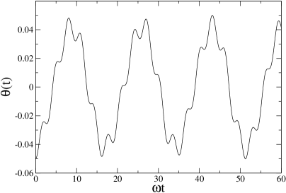
Figure 2: In the linearized classical hydrodynamics approximation, angle of the long axis of the condensate with the $x$ axis of the trap, as a function of time, after the stationary density profile was turned abruptly by a small angle. Here $\epsilon=0.025$ and $\Omega=0.8\omega$. No low frequency oscillation appears: the main oscillation frequency is $\sim 0.37\omega$, in agreement with the lowest frequency of the $\epsilon=0$ limit given by Eq.(14).

III Rotational symmetry breaking: from Goldstone mode to scissors mode

Having failed to find the scissors mode of section I using the classical hydrodynamics approximation we now discard it and turn to a quantum treatment of the problem. Consider a stationary solution of the Gross-Pitaevskii equation with a vortex lattice present, in the case of an isotropic trap, $\epsilon=0$. This solution clearly breaks the rotational symmetry SO(2) of the Hamiltonian. Since this is a continuous symmetry group, Goldstone’s theorem guarantees us the existence of a degree of freedom behaving as a massive boson Blaizot . In particular, this implies the existence of a zero energy eigenmode of the condensate, corresponding to the rotation of the wave function in real space. The “mass” of the Goldstone boson can be shown to be

$$M=\partial_{\Omega}\int\psi^{*}L_{z}\psi.$$ (21)

The variable $\theta$ conjugate to the Goldstone momentum $P$ has the physical meaning of being a rotation angle of the lattice with respect to a reference direction. Note that a quantum spreading of this angular variable takes place when time proceeds, as a consequence of the Goldstone Hamiltonian $P^{2}/2M$.

Now, for a non-zero value of the trap anisotropy, there is no SO(2) symmetry any longer in the Hamiltonian, so that the Goldstone mode is turned into a regular mode of the condensate, behaving as a harmonic oscillator with a finite frequency. This means that the variable $\theta$ now experiences a potential. An intuitive estimate of this potential is obtained by taking the stationary solution, rotating it by an angle $\theta$ and calculating its Gross-Pitaevskii energy in the presence of a trap anisotropy:

$${\cal H}=\frac{P^{2}}{2M}+V(\theta)$$ (22)

where we keep only the $\theta$ dependent part of the energy:

$$V(\theta)=\frac{1}{2}m\omega^{2}\epsilon\left[\langle x^{2}-y^{2}\rangle(1-\cos 2\theta)+2\langle xy\rangle\sin 2\theta\right]$$ (23)

where $\langle\ldots\rangle=\int\psi^{*}\ldots\psi$. We note in passing that the fact that $\psi$ is a local minimum of energy imposes that $V(\theta)\geq 0$ for all rotation angle $\theta$ so that

$$\langle xy\rangle = 0$$ (24)

$$\langle x^{2}-y^{2}\rangle \geq 0.$$ (25)

Quadratising $V(\theta)$ around $\theta=0$ leads to the prediction that the angle $\langle\theta\rangle$ oscillates when initially its value is different from zero. The resulting motion of the condensate is an oscillation of the lattice as a whole, i. e. a scissors mode with an angular frequency:

$$\nu_{\rm scissors}^{2}\simeq\epsilon\frac{2m\omega^{2}\langle x^{2}-y^{2}\rangle}{\partial_{\Omega}\langle L_{z}\rangle}.$$ (26)

This results in a $\sqrt{\epsilon}$ dependence of the mode frequency in the case when $\langle x^{2}-y^{2}\rangle$ does not vanish in the low $\epsilon$ limit.

It is now clear why classical hydrodynamics does not exhibit this low energy mode: since it does not break SO(2) symmetry, the corresponding Goldstone mode is absent and so the low energy scissors mode does not appear. We note that, in cases where SO(2) symmetry breaking would occur in the hydrodynamics equations, the scissors mode frequency would be predicted to tend to zero, even if the motion of the particles is not quantized; this was indeed shown by an explicit solution of the superfluid hydrodynamic equation for a rotating vortex-free condensate exhibiting rotational symmetry breaking and the $\sqrt{\epsilon}$ dependence of the scissors mode frequency was seen experimentally Jean_et_Sandro .

IV Analytical results from Bogoliubov theory

IV.1 Technicalities of Bogoliubov theory

A systematic way of calculating the eigenfrequencies of the condensate is simply to linearize the time dependent Gross-Pitaevskii equation around a stationary solution, taking as unknown the vector $(\delta\psi,\delta\psi^{*})$ where $\delta\psi$ is the deviation of the field from its stationary value. One then faces the following operator,

$${\cal L}_{\rm GP}=\begin{pmatrix}-\frac{\hbar^{2}}{2m}\Delta+U+2g|\psi|^{2}-\Omega L_{z}-\mu&g\psi^{2}\\ -g\psi^{*2}&-\left[-\frac{\hbar^{2}}{2m}\Delta+U+2g|\psi|^{2}-\Omega L_{z}-\mu\right]^{*}\end{pmatrix}$$ (27)

where the complex conjugate of an operator $X$ is defined as $\langle\mathbf{r}|X^{*}|\mathbf{r}^{\prime}\rangle=\langle\mathbf{r}|X|\mathbf{r}^{\prime}\rangle^{*}$. The scissors mode we are looking for is an eigenstate of this operator, and the corresponding eigenvalue over $\hbar$ gives the frequency of the mode.

At this stage, a technical problem appears, coming from the fact that the operator ${\cal L}_{\rm GP}$ is not diagonalizable CastinDum . This can be circumvented by using the number-conserving Bogoliubov theory, in which the eigenmodes of the condensate are the eigenvectors of the following operator:

$${\cal L}=\begin{pmatrix}Q&0\\ 0&Q^{*}\end{pmatrix}{\cal L}_{\rm GP}\begin{pmatrix}Q&0\\ 0&Q^{*}\end{pmatrix}$$ (28)

where $Q$ projects orthogonally to the condensate wave function

$$\phi=\frac{\psi}{N^{1/2}},$$ (29)

and $Q^{*}$ therefore projects orthogonally to $\phi^{*}$. We shall assume here that the operator ${\cal L}$ is diagonalizable for non-zero values of the trap anisotropy $\epsilon$. We shall see in the next subsection that it is in general not diagonalizable for $\epsilon=0$ when several vortices are present.

One then introduces the eigenmodes of $\cal L$, written as $(u_{k},v_{k})$, such that $\int|u_{k}|^{2}-|v_{k}|^{2}=1$; to each of these eigenmodes of eigenvalue $\epsilon_{k}$ corresponds an eigenmode of $\cal L$ of eigenvalue $-\epsilon_{k}^{*}$, given by $(v_{k}^{*},u_{k}^{*})$ Houches . We shall assume here that the condensate wave function is a dynamically stable solution of the stationary Gross-Pitaevskii equation, so that all the $\epsilon_{k}$ are real. We shall also assume that the condensate wave function is a local minimum of the Gross-Pitaevskii energy functional (condition of thermodynamical metastability) so that all the $\epsilon_{k}$ are positive.

IV.2 An upper bound for the lowest energy Bogoliubov mode

We can then use the following result. For a given deviation $\delta\psi^{*}$ of the condensate field from its stationary value, we form the vectors

$$\vec{e}_{q}\equiv{\cal L}^{q}\begin{pmatrix}Q\delta\psi\\ Q^{*}\delta\psi^{*}\end{pmatrix}$$ (30)

where $q$ is an integer. As shown in the appendix A we then have the following inequality:

$$\mathrm{min}_{k}\,\epsilon_{k}\leq\left(\frac{\langle\vec{e}_{0},\vec{e}_{1}\rangle}{\langle\vec{e}_{0},\vec{e}_{-1}\rangle}\right)^{1/2}$$ (31)

where the scalar product $\langle,\rangle$ is of signature $(1,-1)$:

$$\langle\begin{pmatrix}u\\ v\end{pmatrix},\begin{pmatrix}u^{\prime}\\ v^{\prime}\end{pmatrix}\rangle=\int u^{*}u^{\prime}-v^{*}v^{\prime}.$$ (32)

We apply this inequality, taking for $\delta\psi$ the deviation originating from the rotation of $\psi$ by an infinitesimal angle: expanding Eq.(3) to first order in the rotation angle, we put

$$\vec{e}_{0}=\begin{pmatrix}iQL_{z}\psi\\ -iQ^{*}L_{z}^{*}\psi^{*}\end{pmatrix}.$$ (33)

After lengthy calculations detailed in the appendix A, we obtain the upper bound

$$\mathrm{min}_{k}\,\epsilon_{k}^{2}\leq\frac{\hbar^{2}\langle\phi|(\partial_{\theta}^{2}U)|\phi\rangle}{\partial_{\Omega}(\langle\phi|L_{z}|\phi\rangle)}$$ (34)

where $\theta$ is the angle of polar coordinates in the $x-y$ plane.

In the limit of a small $\epsilon$, we assume that the scissors mode is the lowest energy Bogoliubov mode, as motivated in section III. Eq.(34) then gives an upper bound to the scissors mode frequency. An explicit calculation of $\partial_{\theta}^{2}U$ shows that the upper bound Eq.(34) coincides with the intuitive estimate Eq.(26):

$$\partial_{\theta}^{2}U=2m\omega^{2}\epsilon\langle\phi|x^{2}-y^{2}|\phi\rangle.$$ (35)

This upper bound suggests two possibilities in the low $\epsilon$ limit. In the first one, $\langle\phi|x^{2}-y^{2}|\phi\rangle$ tends to a non-zero value, which implies that the scissors mode frequency vanishes at most as $\epsilon^{1/2}$. In the second possibility, $\langle\phi|x^{2}-y^{2}|\phi\rangle$ tends to zero; under the reasonable assumption of a $\langle\phi|x^{2}-y^{2}|\phi\rangle$ vanishing linearly with $\epsilon$, this implies a scissors mode frequency vanishing at most as $\epsilon$. This second case we term ‘degenerate’.

We point out that the degenerate case contains all the cases where the stationary wave function $\psi$ at vanishing trap anisotropy has a discrete rotational symmetry with an angle $\gamma$ different from $\pi$. To show this, we introduce the coordinates rotated by an angle $\gamma$,

$$x^{\prime} = x\cos\gamma-y\sin\gamma$$ (36)

$$y^{\prime} = x\sin\gamma+y\cos\gamma.$$ (37)

The symmetry of $\psi$ implies that $\langle\phi|x^{2}-y^{2}|\phi\rangle=\langle\phi|x^{\prime 2}-y^{\prime 2}|\phi\rangle$ and $\langle\phi|xy|\phi\rangle=\langle\phi|x^{\prime}y^{\prime}|\phi\rangle$. By expansion of these identities, and assuming $1-\cos 2\gamma\neq 0$, one gets $\langle\phi|x^{2}-y^{2}|\phi\rangle=0$.

An important question is to estimate the relative importance of the modes other than the scissors mode excited by the sudden rotation of the condensate. As shown in the appendix A, under the assumption that the scissors mode is the only mode of vanishing frequency when $\epsilon\rightarrow 0$, and anticipating some results of the next subsection, the weight of the initial excitation $\vec{e}_{0}$ on the non-scissors modes behaves as

$$||\vec{e}_{0}^{\,\rm non-scissors}||^{2}=O(\epsilon^{2})$$ (38)

both in the degenerate and the non-degenerate cases.

IV.3 Perturbation theory in $\epsilon$

We now treat the anisotropic part of the trapping potential as a perturbation, $\delta U=m\omega^{2}\epsilon(y^{2}-x^{2})/2$. The Bogoliubov operator $\cal L$, considered as a function of $\epsilon$, can be written as

$${\cal L}_{\epsilon}={\cal L}_{0}+\delta{\cal L}$$ (39)

where $\delta{\cal L}$ is a perturbation. Note that the explicit expression of $\delta{\cal L}$ cannot be given easily, as it involves not only $\delta U$ but also the effect of the first order change of the condensate wave function entering the mean field terms of $\cal L$; but we shall not need such an explicit expression.

Apart from eigenmodes of non-zero eigenfrequency, the operator ${\cal L}_{0}$ has a normal zero energy mode characterized by the vector $\vec{e}_{n}$ and an anomalous mode characterized by the vector $\vec{e}_{a}$, in accordance with Goldstone’s theorem. They are given by

$$\vec{e}_{n} = \begin{pmatrix}Q_{0}L_{z}\psi_{0}\\ -Q_{0}^{*}L_{z}^{*}\psi_{0}^{*}\end{pmatrix}$$ (40)

$$\vec{e}_{a} = \begin{pmatrix}Q_{0}\partial_{\Omega}\psi_{0}\\ Q_{0}^{*}\partial_{\Omega}\psi_{0}^{*}\end{pmatrix}$$ (41)

where $\psi_{0}$ is the stationary condensate field for $\epsilon=0$ and $Q_{0}$ is the projector on the $\epsilon=0$ condensate wavefunction $\phi_{0}$. As shown in the appendix A, one has indeed ${\cal L}_{0}\vec{e}_{n}=0$ and ${\cal L}_{0}\vec{e}_{a}=\vec{e}_{n}$. Within the subspace generated by $\vec{e}_{n}$ and $\vec{e}_{a}$, the operator ${\cal L}_{0}$ has therefore the Jordan canonical form:

$${\cal L}_{0}|_{\rm subspace}=\begin{pmatrix}0&1\\ 0&0\end{pmatrix}.$$ (42)

Note that the normal and the anomalous vectors are, up to a global factor, adjoint vectors for the modified scalar product Eq.(32), in the sense that $\langle\vec{e}_{n},\vec{e}_{a}\rangle=M_{0}$ where $M_{0}$ is given in Eq.(21) for $\epsilon=0$.

As usual in first order perturbation theory, one takes the restriction of the perturbation $\delta{\cal L}$ to the subspace and one then diagonalizes it:

$${\cal L}|_{\rm subspace}=\begin{pmatrix}\delta{\cal L}_{nn}&1+\delta{\cal L}_{na}\\ \delta{\cal L}_{an}&\delta{\cal L}_{aa}\end{pmatrix}.$$ (43)

The notation $\delta{\cal L}_{an}$ means than one takes the component of $\delta{\cal L}\vec{e}_{n}$ onto the vector $\vec{e}_{a}$. Since the adjoint vector of $\vec{e}_{a}$ is $\vec{e}_{n}/M_{0}$ one has

$$\delta{\cal L}_{an}=M_{0}^{-1}\langle\vec{e}_{n},\delta{\cal L}\vec{e}_{n}\rangle.$$ (44)

A similar notation is used for $\delta{\cal L}_{nn}$ and $\delta{\cal L}_{aa}$. Forming the characteristic polynomial of the 2$\times$2 matrix Eq.(43) and taking all the $\delta{\cal L}$’s to be $O(\epsilon)$, one realizes that to leading order in $\epsilon$, the eigenvalues are $\pm\delta{\cal L}_{an}^{1/2}$, that is they scale as $\epsilon^{1/2}$ if $\delta{\cal L}_{an}\neq 0$.

Finally, we use the exact identity $\langle\vec{e_{0}},{\cal L}\vec{e_{0}}\rangle=N\langle\phi|(\partial_{\theta}^{2}U)|\phi\rangle$, proved in the appendix A; noting that $\vec{e}_{n}$ and $\vec{e}_{0}$ differ by terms of first order in $\epsilon$, expanding ${\cal L}$ in ${\cal L}_{0}+\delta{\cal L}$ and using the fact that $\langle\vec{e},{\cal L}_{0}\vec{e}_{n}\rangle=\langle\vec{e}_{n},{\cal L}_{0}\vec{e}\rangle=0$ whatever the vector $\vec{e}$, we get for the scissors mode angular frequency

$$\nu_{\rm scissors}^{2}=\delta{\cal L}_{an}+O(\epsilon^{2})=\frac{\langle\phi_{0}|(\partial_{\theta}^{2}U)|\phi_{0}\rangle}{\partial_{\Omega}\langle\phi_{0}|L_{z}|\phi_{0}\rangle}+O(\epsilon^{2}).$$ (45)

When $\langle x^{2}-y^{2}\rangle_{0}\neq 0$, this coincides with the upper bound Eq.(34) to leading order in $\epsilon$: the upper bound is then saturated for low $\epsilon$.

IV.4 Analytic expressions in the Thomas-Fermi limit for the non-degenerate case

In the Thomas-Fermi limit ($\mu\gg\hbar\omega$) there exist asymptotic functionals giving the energy of the vortex lattice as a function of the vortex positions in the isotropic Dum and anisotropic Aftalion1 cases. Here we shall use these functionals to evaluate the frequency of the scissors mode in Eq.(45).

From the general expression (Eq.(2.12) in Aftalion1 ) we take the simplifying assumption that the distances of the vortex cores to the trap center are much smaller that the Thomas-Fermi radius of the condensate, to obtain

$$\Delta E = \Delta E_{0}+\frac{\eta^{2}m\omega^{2}}{2}\left(\sum_{i}(1-\epsilon)x_{i}^{2}+(1+\epsilon)y_{i}^{2}\right)\left(-2\pi|\log\eta|+2\sqrt{2\pi}\frac{\Omega}{\eta\omega}\right)$$ (46)

$$-\sqrt{2\pi}\hbar\omega\eta\sum_{i\neq j}\log(d_{ij}/l)+O(\epsilon^{2})$$

where $\Delta E$ is the energy difference per atom between the configurations with and without vortices, $\eta=\hbar/\sqrt{2Nmg}=\hbar\omega/(\mu\sqrt{2\pi})\ll 1$ (with $\mu$ being the Thomas-Fermi chemical potential of the non-rotating gas), $(x_{i},y_{i})$ are the coordinates of the i^th vortex core, $d_{ij}$ is the distance between the vortex cores $i$ and $j$ and $l$ is a length scale on the order of the Thomas-Fermi radius and independent of $\epsilon$ tech2 . $\Delta E_{0}$ is a quantity independent of $\epsilon$ and of the vortex positions: therefore we shall not need its explicit expression. It is assumed that $\Omega\ll\omega$, and that

$$\Omega>\Omega_{m}=\left(\frac{\pi}{2}\right)^{1/2}\eta\omega|\log\eta|$$ (47)

i.e. the rotation frequency is large enough to ensure that each vortex experiences an effective trapping potential close to the trap center. An important property of the simplified energy functional is that the positions of the vortices minimizing Eq.(46) are universal quantities not depending on $\Omega$ Aftalion1 when they are rescaled by the length $\lambda$ o_vs_om :

$$\lambda^{2}=\frac{\hbar}{2m(\Omega-\Omega_{m})}.$$ (48)

Now we calculate $\langle x^{2}-y^{2}\rangle$ using the Hellman-Feynman theorem:

$$\frac{d}{d\epsilon}E=-\frac{1}{2}m\omega^{2}\int(x^{2}-y^{2})|\phi|^{2}$$ (49)

where $E$ is the energy per atom and $\phi$ is the condensate wave function. We have also that

$$\frac{d}{d\epsilon}E(\epsilon=0)=\frac{d}{d\epsilon}\Delta E(\epsilon=0)$$ (50)

since the vortex-free configuration is rotationally symmetric for $\epsilon=0$. We thus obtain really_technical

$$\lim_{\epsilon\rightarrow 0}\langle\phi|(x^{2}-y^{2})|\phi\rangle=2\sqrt{2\pi}\eta\frac{\Omega-\Omega_{m}}{\omega}\sum_{i}x^{2}_{i}-y^{2}_{i}.$$ (51)

Using this formula we study vortex lattices with up to ten vortices. By considering first the case $\epsilon=0$, we find that they are all degenerate except the case of two, nine and ten vortices, see figure 3a for $n_{v}=9$ and figure 3b for $n_{v}=10$. Interestingly the $\epsilon=0$ 10-vortex configuration differs from the one of the full numerical simulation of figure 1. By minimizing the simplified energy functional for a non-zero $\epsilon$, we find that the 10-vortex configuration of figure 1 ceases indeed to be a local minimum of energy when $\epsilon$ is smaller than 0.0182: this prevents us from applying Eq.(45) of perturbation theory to the calculation of the scissors mode frequency of the numerical simulations. The 10-vortex configuration of figure 3b ceases to be a local minimum of energy when $\epsilon$ is larger than 0.0173. The 10-vortex configuration minimizing the energy for $0.0173<\epsilon<0.0182$ is a distorted configuration which breaks both the $x$ and $y$ reflection symmetries of the energy functional, but not the parity invariance, see figure 3c.

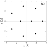
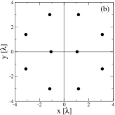
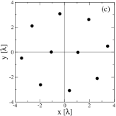
Figure 3: Using the simplified energy functional Eq.(46) we find the minimum energy configurations of nine vortices (a) and ten vortices (b) for $\epsilon=0$. These configurations are non-degenerate: $\sum_{i}(x_{i}^{2}-y_{i}^{2})/\sum_{i}(x_{i}^{2}+y_{i}^{2})\simeq 0.03$ for both of them. For $0.0173<\epsilon<0.0182$ a cross-over takes place between the 10-vortex configuration of (a) and the one of figure 1: such a cross-over configuration is shown in (c), for $\epsilon=0.018$.

The last point is to calculate the derivative of the mean angular momentum with respect to $\Omega$. In the Thomas-Fermi limit, for $\epsilon=0$, and to first order in the squared distance of the vortex cores from the trap center, the angular momentum is given by Dum ; Aftalion1 :

$$\lim_{\epsilon\rightarrow 0}\langle L_{z}\rangle\simeq\hbar n_{v}-\sqrt{2\pi}m\omega\eta\sum_{i}x_{i}^{2}+y_{i}^{2},$$ (52)

where $n_{v}$ is the number of vortices. Using the rescaling by $\lambda$ to isolate the $\Omega$ dependence we get

$$\frac{d}{d\Omega}\langle L_{z}\rangle(\epsilon=0)=-\sqrt{2\pi}{m\omega\eta}\frac{d\lambda^{2}/d\Omega}{\lambda^{2}}\sum_{i}x_{i}^{2}+y_{i}^{2}$$ (53)

where $d\lambda^{2}/d\Omega=-\lambda^{2}/(\Omega-\Omega_{m})<0$. In this way, $\nu_{\rm scissors}$ for low $\epsilon$ can be calculated from Eq.(45) in the non-degenerate case analytically in terms of the equilibrium positions of the vortices:

$$\nu_{\rm scissors}^{2}=4\epsilon(\Omega-\Omega_{m})^{2}\frac{\sum_{i}x_{i}^{2}-y_{i}^{2}}{\sum_{i}x_{i}^{2}+y_{i}^{2}}.$$ (54)

IV.5 Numerical results in the degenerate case

In the degenerate case we must go to higher order in perturbation theory to get the leading order prediction for the frequency of the scissors mode. A simpler alternative is to calculate numerically the frequency of this mode by iterating the operator ${\cal L}^{-1}$ Brachet starting with the initial guess $\vec{e}_{0}$ defined in Eq.(33) tech . The corresponding numerical results are presented in figure 4 in the non-degenerate case of two vortices, and in figure 5 in the degenerate case of three vortices. In the non-degenerate case, $\nu_{\rm scissors}^{2}$ is found to scale linearly with $\epsilon$ for low $\epsilon$, as expected, and the corresponding slope is is very good agreement with the prediction Eq.(45); the agreement with the asymptotic formula Eq.(54) is poor, which could be expected since the parameters are not deeply enough in the Thomas-Fermi regime o_vs_om . In the degenerate case with three vortices, we find numerically that $\nu_{\rm scissors}$ scales as $\epsilon^{3/2}$ for low $\epsilon$, which is indeed compatible with Eq.(34) which leads to a scissor frequency upper bound scaling as $\epsilon$. The fact that a strictly higher exponent ($3/2>1$) is obtained shows that some cancellation happens in the next order of perturbation theory, may be due to the threefold symmetry of the vortex configuration.

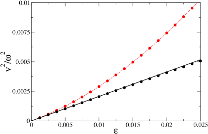
Figure 4: Frequency squared of the scissors mode as a function of the trap anisotropy $\epsilon$ for a condensate with two vortices. $N=2500$, $\Omega=0.6\omega$ and $g=0.0343\hbar^{2}/m$ resulting in a chemical potential $\mu\simeq 4.9\hbar\omega$. The black circles are determined from the iteration of the operator ${\cal L}^{-1}$. The red disks correspond to the numerical evaluation of the upper bound Eq.(34). The solid line corresponds to perturbation theory: it is the numerical evaluation of the leading term in $\epsilon$ of Eq.(45), which is linear in $\epsilon$ with a non-zero slope since the two-vortex configuration is non-degenerate. The red dashed line is a guide to the eyes.

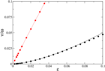
Figure 5: Frequency of the scissors mode as a function of the trap anisotropy $\epsilon$ for a condensate with three vortices. $N=2500$, $\Omega=0.7\omega$ and $g=0.0343\hbar^{2}/m$ resulting in a chemical potential $\mu\simeq 4.6\hbar\omega$. The black circles are determined from the iteration of the operator ${\cal L}^{-1}$. The red disks correspond to the numerical evaluation of the upper bound Eq.(34). The result of perturbation theory is not shown, since it vanishes for a degenerate configuration. The black line is given by the equation $\nu=1.582\epsilon^{3/2}$ and results from a fit of the black disks by a power law $\epsilon^{3/2}$ over the interval $\epsilon\leq 0.01$. The red dashed line is a guide to the eyes.

V Conclusion

In this paper we have studied the problem of a non-classical scissors mode of a condensate containing a vortex lattice. In 2D simulations of the Gross-Pitaevskii equation we showed that, when such a condensate experiences a sudden rotation by a small angle of the anisotropic harmonic trapping potential, the orientation of its vortex lattice will undergo very low frequency oscillations of the scissors mode type. Motivated by these numerical results we searched for this mode using the well-known classical hydrodynamics approximation where the condensate density is a smooth function showing no sign of the presence of vortices and where their effect on the velocity field is taken into account through a coarse-grained vorticity. We showed that this approximation does not contain a low energy scissors mode. We then were able to explain this discrepancy using the Gross-Pitaevskii equation that treats quantum mechanically the motion of the particles. In this case, the density profile of the vortex lattice breaks the rotational symmetry which naturally gives rise to a Goldstone mode in the limit of an isotropic trap and, for a finite anisotropy it becomes a low energy scissors mode. The existence of a scissors mode at a low value of the mode frequency is therefore a direct consequence of the discrete nature of the vortices in a condensate, which is itself a consequence of the quantization of the motion of the particles.

We obtained quantitative predictions for the mode frequency using two separate methods. First we calculated an upper bound on the frequency of the mode using an inequality involving the Bogoliubov energy spectrum. Second, using perturbation theory in $\epsilon$, the anisotropy of the trapping harmonic potential, we showed that this inequality becomes an equality to leading order in $\epsilon$ when the expectation value $\langle x^{2}-y^{2}\rangle_{0}$ taken in the unperturbed state does not vanish; in this case the frequency of the scissors mode tends to zero as $\epsilon^{1/2}$, and we gave an analytic prediction for the coefficient in front of $\epsilon^{1/2}$ in the Thomas-Fermi limit. However, in the cases where the expectation value does vanish (which we termed “degenerate”), the frequency will be at most linear in $\epsilon$. We have illustrated this using a three-vortex lattice where the frequency vanishes as $\epsilon^{3/2}$. Also, in the general case, we have shown that the relative weight of the non-scissors modes excited by a sudden infinitesimal rotation of the trap tends to zero as $O(\epsilon^{2})$ so that the excitation procedure produces a pure scissors mode in the low trap anisotropy limit.

Finally we point out that the existence of the non-classical scissors mode does not rely on the fact that we are dealing with a Bose-Einstein condensate per se. In particular, we expect, based on the very general arguments of section III, that this mode will equally be present in a Fermi superfluid containing a vortex lattice and that its frequency will tend to zero as $\sqrt{\epsilon}$ in the non-degenerate case just like in its bosonic counterpart.

Laboratoire Kastler Brossel is a research unit of Ecole normale supérieure and Université Paris 6, associated to CNRS. This work is part of the research program on quantum gases of the Stichting voor Fundamenteel Onderzoek der Materie (FOM), which is financially supported by the Nederlandse Organisatie voor Wetenschappelijk Onderzoek (NWO).

Appendix A Derivation of the upper bound on the Bogoliubov energies

In this appendix, we prove several results used to control analytically the frequency and the excitation weight of the scissors mode.

We first demonstrate the inequality Eq.(31). The key assumption is that the the condensate wavefunction is a local minimum of energy and does not break any continuous symmetry (which implies here a non-zero trap anisotropy $\epsilon\neq 0$). Then the Bogoliubov operator $\cal L$ of the number-conserving Bogoliubov theory is generically expected to be diagonalizable, with all eigenvalues being real and non-zero. We then expand $\vec{e}_{0}$ on the eigenmodes of $\cal L$:

$$\vec{e}_{0}=\sum_{k\in{\cal F}_{+}}b_{k}\begin{pmatrix}u_{k}\\ v_{k}\end{pmatrix}+b_{k}^{*}\begin{pmatrix}v_{k}^{*}\\ u_{k}^{*}\end{pmatrix}$$ (55)

where ${\cal F}_{+}$ is the set of modes normalized as $\int|u_{k}|^{2}-|v_{k}|^{2}=1$, and which have here strictly positive energies $\epsilon_{k}>0$ since the condensate wavefunction is a local minimum of energy Houches . The $b_{k}$’s are complex numbers; the amplitudes on the modes of the ${\cal F}_{-}$ family (of energies $-\epsilon_{k}$) are simply $b_{k}^{*}$ since $\vec{e}_{0}$ is of the form $(f,f^{*})$. Using the fact that for the modified scalar product Eq.(32), different eigenmodes are orthogonal, and each eigenmode has a ‘norm squared’ equal to $+1$ for ${\cal F}_{+}$ and $-1$ for ${\cal F}_{-}$, we get:

$$\frac{\langle\vec{e}_{0},\vec{e}_{1}\rangle}{\langle\vec{e}_{0},\vec{e}_{-1}\rangle}=\frac{\sum_{k\in{\cal F}_{+}}2\epsilon_{k}|b_{k}|^{2}}{\sum_{k\in{\cal F}_{+}}2\epsilon_{k}^{-1}|b_{k}|^{2}}.$$ (56)

This is simply the expectation value of $\epsilon_{k}^{2}$ with the positive weights $\epsilon_{k}^{-1}|b_{k}|^{2}$. Hence Eq.(31).

Next, starting from $\vec{e}_{0}$ given by Eq.(33), we have to calculate $\vec{e}_{-1}$ and $\vec{e}_{1}$ to obtain Eq.(34).

To calculate $\vec{e}_{-1}$, we take the derivative of the Gross-Pitaevskii equation Eq.(2) with respect to the rotation frequency $\Omega$, which leads to

$${\cal L}_{\rm GP}\begin{pmatrix}\partial_{\Omega}\psi\\ \partial_{\Omega}\psi^{*}\end{pmatrix}=(\partial_{\Omega}\mu)\begin{pmatrix}\psi\\ -\psi^{*}\end{pmatrix}+\begin{pmatrix}L_{z}\psi\\ -L_{z}^{*}\psi^{*}\end{pmatrix}.$$ (57)

We have to get $\cal L$ instead of ${\cal L}_{\rm GP}$: since $\psi$ is normalized to the number of particles $N$, which does not depend on $\Omega$, we have

$$\int\psi^{*}\partial_{\Omega}\psi=i\gamma$$ (58)

where $\gamma$ is real, so that $\partial_{\Omega}\psi=i\gamma\psi/N+Q(\partial_{\Omega}\psi)$ where $Q$ projects orthogonally to $\psi$. Using the fact that $(\psi,-\psi^{*})$ is in the kernel of ${\cal L}_{\rm GP}$, we obtain:

$$\vec{e}_{-1}=\begin{pmatrix}iQ(\partial_{\Omega}\psi)\\ iQ^{*}(\partial_{\Omega}\psi^{*})\end{pmatrix}$$ (59)

which allows to get

$$\langle\vec{e}_{0},\vec{e}_{-1}\rangle=\partial_{\Omega}\int\psi^{*}L_{z}\psi.$$ (60)

In passing, we note that the fact that all $\epsilon_{k}$ are positive implies that $\langle\vec{e}_{0},\vec{e}_{-1}\rangle>0$ so that the mean angular momentum is an increasing function of $\Omega$, a standard thermodynamic stability constraint for a system in contact with a reservoir of angular momentum Rokhsar .

We now proceed with the calculation of $\vec{e}_{1}\equiv{\cal L}\vec{e}_{0}$. Since $L_{z}$ is hermitian,

$$L_{z}\psi=Q(L_{z}\psi)-\alpha\psi$$ (61)

where $\alpha$ is real. Since $(\psi,-\psi^{*})$ is in the kernel of ${\cal L}_{\rm GP}$, we conclude that

$${\cal L}_{\rm GP}\vec{e}_{0}=i\left[{\cal L}_{\rm GP},\begin{pmatrix}L_{z}&0\\ 0&L_{z}^{*}\end{pmatrix}\right]\begin{pmatrix}\psi\\ -\psi^{*}\end{pmatrix}$$ (62)

where $[,]$ stands for the commutator. One calculates the commutator and then computes its action on $(\psi,-\psi^{*})$: various simplifications occur so that

$${\cal L}_{\rm GP}\vec{e}_{0}=\begin{pmatrix}-\hbar(\partial_{\theta}U)\psi\\ \hbar(\partial_{\theta}U)\psi^{*}\end{pmatrix}$$ (63)

where $\theta$ is the angle of polar coordinates in the $x-y$ plane and where we used $L_{z}=-i\hbar\partial_{\theta}$. $\vec{e}_{1}$ results from this expression by projection. We finally obtain

$$\langle\vec{e}_{0},\vec{e}_{1}\rangle=\hbar^{2}\int\psi^{*}(\partial_{\theta}^{2}U)\psi.$$ (64)

In what concerns the scissors mode frequency, the last point is to justify the identities ${\cal L}_{0}\vec{e}_{n}=0$ and ${\cal L}_{0}\vec{e}_{a}=\vec{e}_{n}$, where ${\cal L}_{0}$ is the $\epsilon=0$ limit of ${\cal L}$, $\vec{e}_{n}$ is defined in Eq.(40) and $\vec{e}_{a}$ is defined in Eq.(41). First, one notes that, within a global factor $i$, $\vec{e}_{n}$ is the limit of $\vec{e}_{0}$ for $\epsilon\rightarrow 0$. Then taking the limit $\epsilon\rightarrow 0$ in Eq.(63), one immediately gets ${\cal L}_{0}\vec{e}_{n}=0$ since $\partial_{\theta}U$ vanishes when the trapping potential $U$ is rotationally symmetric. Second, one notes from Eq.(59) that, within a global factor $i$, $\vec{e}_{a}$ is the zero $\epsilon$ limit of $\vec{e}_{-1}$. Then taking the zero $\epsilon$ limit of the identity ${\cal L}\vec{e}_{-1}=\vec{e}_{0}$ leads to ${\cal L}_{0}\vec{e}_{a}=\vec{e}_{n}$.

Finally we control the weight of the modes other than the scissors mode that are excited by the sudden infinitesimal rotation of the condensate:

$$||\vec{e}_{0}^{\,\rm non-scissors}||^{2}\equiv||\sum_{k\in{\cal F}_{+}\setminus\{k_{s}\}}b_{k}\begin{pmatrix}u_{k}\\ v_{k}\end{pmatrix}+b_{k}^{*}\begin{pmatrix}v_{k}^{*}\\ u_{k}^{*}\end{pmatrix}||^{2}$$ (65)

where $||\ldots||$ is the usual ${\cal L}_{2}$ norm and $k_{s}$ is the index of the scissors mode. The basic assumption is that the scissors mode is the only one with vanishing frequency in the $\epsilon\rightarrow 0$ limit. We rewrite Eq.(64) as

$$\sum_{k\in{\cal F}_{+}}2\epsilon_{k}|b_{k}|^{2}=2m\omega^{2}\epsilon\int(x^{2}-y^{2})|\psi|^{2}.$$ (66)

In the degenerate case the right-hand side is $O(\epsilon^{2})$ so that each (positive) term $\epsilon_{k}|b_{k}|^{2}$ is $O(\epsilon^{2})$. For the normal modes, both $\epsilon_{k}^{-1}$ and the mode functions $u_{k},v_{k}$ have a finite limit for $\epsilon\rightarrow 0$, which proves $||\vec{e}_{0}^{\,\rm non-scissors}||^{2}=O(\epsilon^{2})$.

In the non-degenerate case the same reasoning leads to a weight being $O(\epsilon)$. A better estimate can be obtained from

$$\langle\vec{e}_{0},\vec{e}_{1}\rangle-\epsilon_{k_{s}}^{2}\langle\vec{e}_{0},\vec{e}_{-1}\rangle=\sum_{k\in{\cal F}_{+}\setminus\{k_{s}\}}2\left(\epsilon_{k}-\epsilon_{k_{s}}^{2}/\epsilon_{k}\right)|b_{k}|^{2}.$$ (67)

Then using the explicit expression for the scalar products in the left-hand side, see Eq.(60) and Eq.(64), and using the result Eq.(45) of the perturbative expansion for $\nu_{\rm scissors}=\epsilon_{k_{s}}/\hbar$, one realizes that the left-hand side of Eq.(67) is $O(\epsilon^{2})$, which leads to a weight on non-scissors modes being $O(\epsilon^{2})$ as in the degenerate case.

References

- (1) M.H. Anderson, J.R. Ensher, M.R. Matthews, C.E. Wieman, and E.A. Cornell, Science 269, 198 (1995).
- (2) K. B. Davis, M. O. Mewes, M. R. Andrews, N. J. van Druten, D. D. Durfee, D. M. Kum, and W. Ketterle, Phys. Rev. Lett. 75, 3969 (1995).
- (3) W. Ketterle, D. S. Durfee, and D. M. Stamper-Kurn, “Making, probing and understanding Bose-Einstein condensates” in Bose-Einstein Condensation in Atomic Gases, M. Inguscio, S. Stringari, and C. E. Wieman (Eds.), IOS Press, Amsterdam, pp. 67-176 (1999).
- (4) F. Dalfovo, S. Giorgini, L. P. Pitaevskii, and S. Stringari, Rev. of Mod. Phys. 71, 463 (1999).
- (5) N. Lo Iudice and F. Palumbo, Phys. Rev. Lett. 41, 1532 (1978); E. Lipparini and S. Stringari, Phys. Lett. B 130, 139 (1983).
- (6) D. Guéry-Odelin and S. Stringari, Phys. Rev. Lett. 83, 4452 (1999).
- (7) O.M. Maragò, S. Hopkins, J. Arlt, E. Hodby, G. Hechenblaikner, and C.J. Foot, Phys. Rev. Lett. 84, 2056 (2000).
- (8) K. W. Madison, F. Chevy, W. Wohlleben, and J. Dalibard, Phys. Rev. Lett. 84, 806 (2000).
- (9) J. R. Abo-Shaeer, C. Raman, J. M. Vogels, and W. Ketterle, Science 292, 476 (2001).
- (10) P. C. Haljan, I. Coddington, P. Engels, and E. A. Cornell, Phys. Rev. Lett. 87, 210403 (2001).
- (11) C. Lobo, A. Sinatra, and Y. Castin Phys. Rev. Lett. 92, 020403 (2004).
- (12) E. B. Sonin, Rev. Mod. Phys. 59, 87 (1987).
- (13) Quasi 2D means that the motion of the gas along is frozen in the ground state of a trapping potential, but still the -wave scattering length remains much smaller than the spatial width of the gas along so that the scattering of two atoms does not acquire a true 2D character.
- (14) Y. Castin, and R. Dum, Eur. Phys. J. D 7, 399 (1999).
- (15) M. Modugno, L. Pricoupenko, and Y. Castin, Eur. Phys. J. D 22, 235 (2003).
- (16) M. Cozzini and S. Stringari, Phys. Rev. A 67, 041602 (2003).
- (17) This shows that the zero frequency mode predicted by classical hydrodynamics is not the scissors mode of the classical hydrodynamics. Anticipating the quantum treatment of the problem, one can show that for , the zero frequency mode of the classical hydrodynamics actually corresponds to the anomalous mode of the quantum theory.
- (18) J.P. Blaizot and G. Ripka Quantum Theory of Finite Systems (The MIT Press, 1985).
- (19) M. Cozzini, S. Stringari, V. Bretin, P. Rosenbusch, and J. Dalibard, Phys. Rev. A 67, 021602 (2003).
- (20) Y. Castin and R. Dum, Phys. Rev. A 57, 3008-3021 (1998).
- (21) Y. Castin, pp. 1-136, “Bose-Einstein Condensates in Atomic Gases: Simple Theoretical Results” in Coherent atomic matter waves, Lecture notes of Les Houches summer school, edited by R. Kaiser, C. Westbrook, and F. David, EDP Sciences and Springer-Verlag (2001).
- (22) A. Aftalion and Q. Du, Phys. Rev. A 64, 063603 (2001).
- (23) The argument of the logarithm is not calculated in Aftalion1 but in Aftalion2 where it is done for the 3D case. Converting this calculation to 2D, we find that the argument does not depend on to first order.
- (24) A. Aftalion and T. Rivière, Phys. Rev. A 64, 043611 (2001).
- (25) The condition that are much smaller than the Thomas-Fermi radius, combined with the sum rule Aftalion1 for the steady state positions, implies that is smaller than the Thomas-Fermi radius, which leads to the condition .
- (26) If one keeps to first order the position dependence of the prefactor of the in Aftalion1 , one gets an extra contribution on the right hand side of Eq.(51), given by . We have checked for and that it is indeed negligible under the condition derived in o_vs_om .
- (27) C. Huepe, S. Metens, G. Dewel, P. Borckmans, and M. E. Brachet, Phys. Rev. Lett. 82, 1616 (1999).
- (28) The procedure is as follows: we wish to find such that . It then follows that we need only minimize the quantity where since is a positive definite matrix (because is a local minimum of the Gross-Pitaevskii energy functional) whereas is not. We then perform the minimization numerically using the conjugate gradient method.
- (29) D. A. Butts and D. S. Rokhsar, Nature 397, 327 (1999).