Chaos, Coherence and the Double-Slit Experiment

Abstract

We investigate the influence that classical dynamics has on interference patterns in coherence experiments. We calculate the time-integrated probability current through an absorbing screen and the conductance through a doubly connected ballistic cavity, both in an Aharonov-Bohm geometry with forward scattering only. We show how interference fringes in the probability current generically disappear in the case of a chaotic system with small openings, and how they may persist in the case of an integrable cavity. Simultaneously, the typical, sample dependent amplitude of the flux-sensitive part $g(\phi)$ of the conductance survives in all cases, and becomes universal in the case of a chaotic cavity. In presence of dephasing by fluctuations of the electric potential in one arm of the Aharonov-Bohm loop, we find an exponential damping of the flux-dependent part of the conductance, $g(\phi)\propto\exp[-\tau_{\rm L}/\tau_{\varphi}]$, in term of the traversal time $\tau_{\rm L}$ through the arm and the dephasing time $\tau_{\varphi}$. This extends previous works on dephasing in ballistic systems to the case of many conducting channels.

I Introduction

Ever since the inception of quantum theory, questions have been raised related to its connection to classical physics wheeler83 . From a dynamical point of view, it is generally accepted that the Liouville and Schrödinger equations deliver the same time-evolution for short enough times, $t<t_{\rm E}$. In both chaotic and integrable dynamical systems, $t_{\rm E}$ goes to infinity in the semiclassical limit of large quantum numbers. In chaotic systems, however, the quantum breaktime $t_{\rm E}=\lambda^{-1}|\ln\hbar_{\rm eff}|$ does so only logarithmically slowly in the effective Planck’s constant $\hbar_{\rm eff}$ ($\lambda$ is the system’s Lyapunov exponent) berman78 . For $t>t_{\rm E}$, the standard view is that external sources of decoherence have to be invoked in order to reestablish the correspondence between quantum and classical mechanics aak ; joos ; caldeira85 ; buttiker86a .

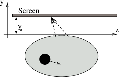
Figure 1: (a) Double-slit set-up of Ref. casati04 . A cavity is pierced by two slits. A wavepacket of well resolved initial momentum is prepared inside the cavity and leaks out little by little. The current through a screen is measured and integrated over time.

Arguing that the necessity of external degrees of freedom for the quantum to classical transition remains unclear (see for instance Ref.casati95 ), Casati and Prosen recently performed a numerical double-slit experiment casati04 . The set-up they considered is sketched in Fig. 1. One pierces two openings of width $W$ in an otherwise closed cavity. Inside the cavity, a particle of mass $m\equiv 1$ is prepared in an initial wavepacket of minimal spread in momentum. The system is considered to be semiclassical, i.e. the ratio of the linear system size and the particle’s de Broglie wavelength is big $L/\nu=kL/2\pi\gg 1$. As time goes by, the particle leaks out of the cavity with an average decay time $\tau_{d}\propto L^{2}/(Wv)\gg\tau_{\rm f}$ much larger than the time of flight $\tau_{\rm f}\equiv L/v$ across the cavity, $v$ being the particle’s velocity. That is, the particle bounces many times between the cavity’s boundary before exiting. One then records the integrated probability current $I(x)$ through the screen, (from now on we set $\hbar\equiv 1$)

$$I(z) = \int_{0}^{\infty}{\rm d}t\;{\rm Im}[\psi^{*}(z,y;t)\;\partial_{y}\psi(z,y;t)]_{y=y_{\rm o}}.$$ (1)

Two different situations were considered, where the cavity was either integrable (an isosceles right triangle) or chaotic (where the hypotenuse was replaced by a circular arc). In the integrable case, numerics showed that $I(x)$ exhibits the expected interference fringes. Those fringes were however absent in the chaotic case where $I(x)$ takes on its classical, structureless shape. These results prompted Casati and Prosen to draw two conclusions: (i) the double-slit set-up provides for a “vivid and fundamental illustration of the manifestation of classical chaos in quantum mechanics”, and (ii) dynamical chaos alone (i.e. without any external source of noise, or any coupling to an external bath or environment) can produce sufficient randomization of quantum-mechanical phases resulting in a quantum to classical transition in the semiclassical limit. The reasoning path leading to conclusion (ii) is qualitatively the following. Due to the long lifetime of the particle inside the cavity, the wavepacket must hit the cavity walls many times before exiting. Semiclassically, the wavepacket follows many classical trajectories exiting at different times, and thus accumulating different action phases. In the regular case, because the particle’s initial momentum is well defined, the action phases accumulated along all those trajectories are correlated. In the chaotic case however, the initial momentum uncertainty grows exponentially with time and the classical trajectories have a broad, continuous distribution of duration. Hence they acquire a random distribution of action phases. Based on this observation, Casati and Prosen concluded that this phase randomization prevents interference fringes to occur, in agreement with their numerical calculation. It is important to realize at this point that at any given point and time, the phase of the wavefunction is uniquely defined, and can in principle be deterministically obtained from the initial condition.

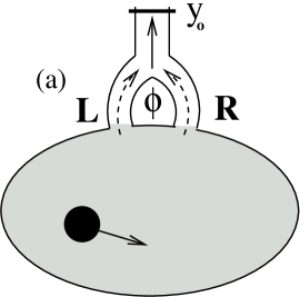
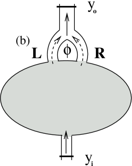
Figure 2: (a) Double-slit set-up similar to that of Ref. casati04 (see Fig. 1). A cavity is pierced by two slits which are connected via an Aharonov-Bohm geometry to a single lead. A wavepacket is prepared inside the cavity and leaks out little by little. The current through a cross-section ${\cal C}$ (located at $y=y_{\rm o}$) of the outgoing lead is measured and integrated over time. (b) Transport set-up. The same cavity as in (a) is connected to an additional current-injection lead. The current through ${\cal C}$ is measured. Taking its ratio with the applied voltage gives the conductance.

There is no controversy related to conclusion (i). Conclusion (ii) however, not only challenges the standard view according to which long-time quantum-classical correspondence requires coupling to external degrees of freedom, but has to be reconciled with well established mesoscopic physics results textbooks . It is indeed well known that both transport aronov87 ; webb85 ; yacoby95 and thermodynamical cheung89 ; vonoppen91 ; levy90 properties of multiply connected mesoscopic samples threaded by a magnetic flux display coherent flux-periodic oscillations of a purely quantal origin. It is doubtful that all experimentally investigated systems are integrable. From a theoretical point of view, such oscillations have been moreover predicted for disordered, diffusive samples with point-like impurities which are arguably as good “phase-randomizers” (in the sense given above) as deterministic chaos. The even flux-harmonics (those having a period in the applied flux $\phi$ of $\phi_{0}/2n$, with $n$ a positive integer and $\phi_{0}=h/e$ the flux quantum) of these oscillations even survive disorder averaging aronov87 ; vonoppen91 , and in the case of transport experiments “à la Sharvin and Sharvin”, the amplitude of the Aharonov-Bohm oscillations of the conductance are mostly insensitive to the amount of disorder aronov87 . Clearly, conductance is insensitive to the “dynamical decoherence” scenario of conclusion (ii). The purpose of this article is to reconcile the numerical experiment of Ref. casati04 with the established theoretical and experimental wisdom of mesoscopic physics, as well as to investigate dephasing in ballistic mesoscopic systems.

We will present a comparative semiclassical calculation of the outgoing probability current in the Aharonov-Bohm two-slit set-up of Fig. 2(a) (similar to the set-up of Ref. casati04 , see Fig. 1) and of the conductance in the set-up of Fig. 2(b). In both cases, a cavity is connected to two intermediate left (L) and right (R) leads carrying $N_{\rm R,L}\gg 1$ transport channels. These intermediate leads eventually merge and the loop they form is threaded by a magnetic flux $\phi$. In the transport set-up of Fig. 2(b), the cavity is in addition connected to a current-injecting lead carrying $N_{\rm B}$ transport channels. In the two instances, we consider ideally connected, i.e. non reflecting leads, and will restrict ourselves to the situation where the number $N_{\rm T}$ of outgoing channels obeys $N_{\rm T}\gtrsim N_{\rm L}+N_{\rm R}$. One can then neglect processes where particles circulate several times around the Aharonov-Bohm loop. As but one consequence, our semiclassical treatment is fully unitary, but flux-dependent weak localization corrections are absent. Such corrections have been considered in a different ballistic set-up in Ref. see03 . The set-up of Fig. 2(b) in the diffusive regime has been considered in Ref. mirlin04 . A nonunitary semiclassical treatment of the set-up of Fig. 2(b) considering backscattering due to pairs of time-reversed paths has been presented in Ref. kawabata96 .

Our conclusion is that, while there is nothing wrong with most of the reasonings and the numerical results of Ref. casati04 , decoherence cannot be claimed to occur when one observable does not display interference patterns, but when this is the case for all possible observables. The conductance experiment of Fig. 2(b) will be shown to exhibit sample-dependent Aharonov-Bohm oscillations in both cases of an integrable and a chaotic cavity. We will see how these oscillations disappear as dephasing is introduced. Our results support the standard wisdom according to which the quantum to classical crossover requires a coupling to external degrees of freedom.

The paper is organized as follows. In Section II we present a semiclassical calculation for an Aharonov-Bohm set-up similar to the two-slit experiment considered in Ref. casati04 . This calculation is extended to the calculation of the conductance in an Aharonov-Bohm transport set-up in Section III. In Section IV we introduce dephasing by means of a fluctuating electric potential in one arm of the Aharonov-Bohm loop, and investigate the associated disappearance of flux-dependent interference fringes. In the final Section V we will summarize our findings and discuss future directions and open questions.

II Two-Slit Set-up

We first consider the Aharonov-Bohm two-slit set-up of Fig. 2(a), where an initial wavepacket is prepared inside the cavity. The latter is connected to two outgoing leads carrying many transverse channels. The leads eventually merge, forming a loop threaded by a magnetic flux $\phi$. Once one integrates over a cross-section of the outgoing lead, the situation is fully similar to Ref. casati04 , with $\phi$ playing the role of the coordinate $z$ along the screen (see Fig. 1). We consider an initial Gaussian wavepacket $\psi_{0}({\bf r}_{1})=(\pi\nu^{2})^{-d/4}\exp[i{\bf p}_{0}\cdot({\bf r}_{1}-{\bf r}_{0})-|{\bf r}_{1}-{\bf r}_{0}|^{2}/2\nu^{2}]$, and approximate its time-evolution semiclassically by ($H=v^{2}/2$; remember that we set $m\equiv 1$)

$$\langle{\bf r}|\exp(-iHt)|\psi_{0}\rangle=\int d{\bf r}_{1}\sum_{s}K_{s}({\bf r},{\bf r}_{1};t)\psi_{0}({\bf r}_{1}),$$ (2a)

$$K_{s}^{H}({\bf r},{\bf r}_{1};t)=C_{s}^{1/2}\exp[iS_{s}({\bf r},{\bf r}_{1};t)-i\pi\mu_{s}/2].$$ (2b)

Compared to Ref. casati04 , the Heisenberg uncertainty is evenly distributed between momentum and spatial coordinates in our choice of an initial state. This should not matter in a chaotic cavity, but may affect the outcome of the experiment in a regular cavity. The semiclassical propagator (2b) is expressed as a sum over classical trajectories (labeled $s$) connecting ${\bf r}$ and ${\bf r}_{1}$ in the time $t$. For each $s$, the partial propagator contains the action integral $S_{s}^{H}({\bf r},{\bf r}_{1};t)$ along $s$, a Maslov index $\mu_{s}$, and the determinant $C_{s}$ of the stability matrix. Because of the cavity openings, if ${\bf r}$ in Eqs. (2) is inside the cavity, then the sum runs only over those classical trajectories that have not yet escaped at time $t$, whereas if ${\bf r}$ lies somewhere in a lead, it runs over the trajectories that went exactly once through either of the openings to reach ${\bf r}$. Here, we are concerned with this latter case, putting ${\bf r}=(x,y=y_{\rm o})$ at the horizontal position $x$ on a cross-section ${\cal C}$ of the outgoing lead defined by $y=y_{\rm o}$ [see Fig. 2(a)]. Later on, we will integrate over $x$.

The semiclassical expression for the time-integrated probability current (1) is given by

$$I(x,\phi) = \frac{v}{(\pi\nu^{2})^{d/2}}\int_{0}^{\infty}{\rm d}t\int{\rm d}{\bf r}_{1}\int{\rm d}{\bf r}_{2}$$ (3)

$$\times \sum_{s(t),s^{\prime}(t)}\;[C_{s}C_{s^{\prime}}]^{1/2}\cos\theta_{s}$$

$$\times \exp\Big{[}i\{S_{s}(x,y_{\rm o};{\bf r}_{1};\phi,t)-S_{s^{\prime}}(x,y_{\rm o};{\bf r}_{2};\phi,t)\}\Big{]}$$

$$\times \exp\Big{[}i\pi(\mu_{s^{\prime}}-\mu_{s})/2\Big{]}\exp\Big{[}i{\bf p}_{0}\cdot({\bf r}_{1}-{\bf r}_{2})\Big{]}$$

$$\times \exp\Big{[}-(|{\bf r}_{1}-{\bf r}_{0}|^{2}+|{\bf r}_{2}-{\bf r}_{0}|^{2})/2\nu^{2}\Big{]},$$

where we used $\partial_{y}S_{s}=v_{y,s}=v\cos\theta_{s}$, with $v_{y,s}$ the velocity in $y$-direction and thus $\theta_{s}$ the angle of incidence, as the path $s$ crosses ${\cal C}$ at time $t$.

The first step in the calculation of $I(x,\phi)$ is to linearize $S_{s}(x,y_{\rm o};{\bf r}_{1};\phi,t)\simeq S_{s}(x,y_{\rm o};{\bf r}_{0};\phi,t)-{\bf p}_{s}\cdot({\bf r}_{1}-{\bf r}_{0})$, with ${\bf p}_{s}$ the initial momentum on path $s$. This is justified by our choice of a narrow initial wavepacket. One it then left with Gaussian integrals over ${\bf r}_{1,2}$. Enforcing a stationary phase condition, the dominant, classical contributions to $I(x,\phi)$ are identified as those with $s=s^{\prime}$. Under our assumption of a final number of transport channels $N_{\rm T}\gtrsim N_{\rm L}+N_{\rm R}$ roughly equal or somehow larger than the sum of transport channels in the intermediate leads forming the Aharonov-Bohm loop, single trajectories do not enclose any flux. Diagonal contributions with $s=s^{\prime}$ are thus flux independent. Writing $I(x,\phi)=I_{0}(x)+I_{\phi}(x)$, one has

$$\langle I_{0}(x)\rangle = v\;(4\pi\nu^{2})^{d/2}$$

$$\times \int_{0}^{\infty}{\rm d}t\sum_{s(t)}\;C_{s}\cos\theta_{s}\exp[-\nu^{2}|{\bf p}_{0}-{\bf p}_{s}|^{2}].$$

The stationary phase leading to the diagonal approximation $s=s^{\prime}$ is justified once one averages over an interval of energy $\delta E$ which is classically small (i.e. which does not modify the trajectories) but quantum-mechanically large (i.e. such that $\delta E\cdot\tau_{d}\gg 1$). This is indicated by brackets in Eq. (II). The average value $\langle I_{0}(x)\rangle$ is calculated under the assumption that the cavity is ergodic, in particular that the wavefunction will eventually leak out of it completely. That is, the time-integrated current through ${\cal C}$ must be equal to one and one has

$$\frac{2v}{\pi}\;\int_{0}^{W}{\rm d}x\int_{0}^{\infty}{\rm d}t\;|\psi(x,y_{\rm o};t)|^{2} =1,$$ (5)

where a factor $2/\pi$ originated from averaging the incidence angle on ${\cal C}$ in the interval $[-\pi/2,\pi/2]$. This provides the semiclassical sum rule

$$v\;(4\pi\nu^{2})^{d/2}\int_{0}^{W}{\rm d}x\int_{0}^{\infty}{\rm d}t$$

$$\times\sum_{s(t)}\;C_{s}\exp[-\nu^{2} |{\bf p}_{0}-{\bf p}_{s}|^{2}]=\pi/2.$$ (6)

The classical time-integrated current through ${\cal C}$ is then obtained as

$$\int_{0}^{W}{\rm d}x\langle I_{0}(x)\rangle = 1.$$ (7)

In the limit of a wide outgoing lead, $W\gg\nu$, the probability current is ergodically distributed over ${\cal C}$ so that the average current per unit length is given by $\langle I_{0}(x)\rangle\approx W^{-1}$.

After this warm-up calculation we turn our attention to the flux-dependent part $I_{\phi}(x)$. It correspond to pairs of paths $s$ and $s^{\prime}$ in Eq. (3) exiting through different arms of the AB ring, and evidently they are not included in the diagonal approximation $s=s^{\prime}$. Furthermore, no stationary phase approximation can be systematically enforced to identify them, which reflects the fact that they vanish on average. That is to say $\langle I_{\phi}(x)\rangle=0$, once it is averaged over different initial conditions, a sufficiently large energy interval or an ensemble of different cavities. This is but one consequence of our choice of forward scattering processes only at the merging point of the intermediate leads.

To investigate the behavior of $I_{\phi}(x)$ for a given cavity and/or initial wavepacket preparation, we proceed to calculate $\langle I^{2}_{\phi}(x)\rangle$, the squareroot of which gives the value of the flux-dependent part of $I(x)$ for a typical experimental realization. Our approach is similar in spirit to the one followed in Ref. cheung89 in the context of persistent currents. A similar sum rule as (II) is helpful in computing $\langle I^{2}_{\phi}(x)\rangle$, and with little extra work we will see that $\langle I^{2}_{\phi}(x)\rangle\propto(1-\exp[-\tau_{\rm erg}/\tau_{d}])^{2}(kL)^{-1}\approx(\tau_{\rm erg}/\tau_{d})^{2}(kL)^{-1}$, where $\tau_{\rm erg}$ is the ergodic time. In a chaotic cavity, it is generally given by few times the time of flight across the cavity, so that $\tau_{\rm erg}/\tau_{d}\propto W/L$. In the numerical experiment of Ref. casati04 , both the ratio of the width of the openings to the linear system size and the inverse semiclassical parameter $kL$ are much smaller than one, inducing the disappearance of the interference fringes.

Noting that $S_{s}(x,y_{\rm o};{\bf r}_{0};\phi,t)=S_{s}(x,y_{\rm o};{\bf r}_{0};t)\pm\pi\phi/\phi_{0}$, where the ${}^{\prime\prime}+^{\prime\prime}$ and ${}^{\prime\prime}-^{\prime\prime}$ signs correspond to trajectories going through the right and the left intermediate lead respectively, linearizing in ${\bf r}_{1,2}-{\bf r}_{0}$ and performing the resulting Gaussian integrals over ${\bf r}_{1,2}$ as above, one has

$$I_{\phi}(x)I_{\phi}(x^{\prime}) = 4v^{2}\;(4\pi\nu^{2})^{d}\cos^{2}[2\pi\phi/\phi_{0}]\;\int_{0}^{\infty}{\rm d}t_{1}\int_{0}^{\infty}{\rm d}t_{2}\;\sum_{s_{1},s_{3}\in L}\sum_{s_{2},s_{4}\in R}\;\left(\;\prod_{i=1}^{4}C_{i}\;\right)^{1/2}\cos\theta_{1}\;\cos\theta_{4}$$ (8)

$$\times \exp\Big{[}i\big{\{}S_{1}(x,y_{\rm o};{\bf r}_{0};t_{1})-S_{2}(x,y_{\rm o};{\bf r}_{0};t_{1})-S_{3}(x^{\prime},y_{\rm o};{\bf r}_{0};t_{2})+S_{4}(x^{\prime},y_{\rm o};{\bf r}_{0};t_{2})\big{\}}\Big{]}$$

$$\times \exp\Big{[}-\nu^{2}\big{\{}|{\bf p}_{0}-{\bf p}_{1}|^{2}+|{\bf p}_{0}-{\bf p}_{2}|^{2}+|{\bf p}_{0}-{\bf p}_{3}|^{2}+|{\bf p}_{0}-{\bf p}_{4}|^{2}\big{\}}/2\Big{]},$$

where we shortened the notation, i.e. $\theta_{i}=\theta_{s_{i}}$, $S_{i}=S_{s_{i}}$ and so forth. It is important to keep in mind that $s_{1}$ and $s_{2}$ exit the cavity after a time $t_{1}$, while the time of escape is $t_{2}$ for the other two trajectories $s_{3}$ and $s_{4}$. Because trajectories exit via two different arms of the AB loop, the only stationary phase condition that can be satisfied is to set $s_{1}=s_{3}$ and $s_{2}=s_{4}$, which then requires to set $x=x^{\prime}$ with accuracy $\nu$, and $t_{1}\approx t_{2}$, with an accuracy given by the time $\tau^{*}\simeq\hbar/E$ necessary for the classical ballistic flow at energy $E$ to accumulate an action $\hbar$. We substitute $\int{\rm d}t_{1}\int{\rm d}t_{2}\rightarrow\tau^{*}\int{\rm d}t_{1}$ to get

$$\langle I_{\phi}(x)I_{\phi}(x^{\prime})\rangle\simeq\delta_{\nu}(x-x^{\prime})\;4v^{2}\tau^{*}\;(4\pi\nu^{2})^{d}\cos^{2}[2\pi\phi/\phi_{0}]\int_{0}^{\infty}{\rm d}t_{1}\;\sum_{s_{1}\in L}\sum_{s_{2}\in R}\;\prod_{i=1}^{2}\Big{\{}C_{i}\cos\theta_{i}\;\exp\big{[}-\nu^{2}|{\bf p}_{0}-{\bf p}_{1}|^{2}\big{]}\Big{\}},$$ (9)

where $\delta_{\nu}(x-x^{\prime})$ enforces the condition $x=x^{\prime}$ with an accuracy ${\cal O}(\nu)$. Because there is only one time integral but two summations over classical paths, one cannot use Eq. (II) directly. Assuming that the system is ergodic, which means in particular that for times long enough, $t\geq\tau_{\rm erg}\approx\tau_{f}$, spatial averages equal time averages, one writes

$$\langle I^{2}_{\phi}(x)\rangle \simeq 4v^{2}\;(4\pi\nu^{2})^{d}\cos^{2}[2\pi\phi/\phi_{0}]\Bigg{[}\tau^{*}\;\int_{0}^{\tau_{\rm erg}}{\rm d}t_{1}\;\sum_{s_{1}\in L}\sum_{s_{2}\in R}\;\prod_{i=1}^{2}\Big{\{}C_{i}\cos\theta_{i}\;\exp\big{[}-\nu^{2}|{\bf p}_{0}-{\bf p}_{1}|^{2}\big{]}\Big{\}}$$ (10)

$$+ \;\int_{\tau_{\rm erg}}^{\infty}{\rm d}t_{1}\lim_{T\rightarrow\infty}\frac{\tau^{*}}{T}\int_{\tau_{\rm erg}}^{T}{\rm d}t_{2}\;\sum_{s_{1}\in L}\sum_{s_{2}\in R}\;\prod_{i=1}^{2}\Big{\{}C_{i}\cos\theta_{i}\;\exp\big{[}-\nu^{2}|{\bf p}_{0}-{\bf p}_{1}|^{2}\big{]}\Big{\}}\Bigg{]}.$$

Here, the second term inside the brackets corresponds to trajectories $s_{1}(t_{1})$ and $s_{2}(t_{2})$ exiting at different times. Its contribution to the integrated current $\int dx\langle I^{2}_{\phi}(x)\rangle$ can be calculated using the sum rule (II) and making the assumption that the current is homogeneously distributed on ${\cal C}$. We find that it vanishes $\propto{\rm lim}_{T\rightarrow\infty}\;\tau^{*}/T$. The first, pre-ergodic term is highly non-universal and we cannot calculate it generically. We can however give an estimate to its amplitude using

$$\;\int_{0}^{\tau_{\rm erg}}{\rm d}t_{1}\;f(t_{1})\;g(t_{1})\sim\tau_{\rm erg}^{-1}\;\int_{0}^{\tau_{\rm erg}}{\rm d}t_{1}\;{\rm d}t_{2}\;f(t_{1})\;g(t_{2})\sim\tau_{\rm erg}^{-1}\;(1-\exp[-\tau_{\rm erg}/\tau_{d}])^{2}\;\int_{0}^{\infty}{\rm d}t_{1}\;{\rm d}t_{2}\;f(t_{1})\;g(t_{2}).$$ (11)

The first relation results from removing the requirement that both trajectories $s_{1}$ and $s_{2}$ in Eq. (10) exit at the same time, and to obtain the second one, we used the measure of pre-ergodic trajectories in an open chaotic cavity $\tilde{\rho}(t\leq\tau_{\rm erg})=\tau_{d}^{-1}\int_{0}^{\tau_{\rm erg}}{\rm d}t\exp[-t/\tau_{d}]$, where $\rho(t)=\tau_{d}^{-1}\exp[-t/\tau_{d}]$ is the distribution of dwell times through a chaotic system Bauer90 . Using $\tau^{*}/\tau_{\rm erg}\simeq(kL)^{-1}$, and assuming again an homogeneous distribution of $I(x)$ on ${\cal C}$, we finally get the typical flux-dependent probability current as

$$\langle I^{2}_{\phi}(x)\rangle^{1/2} \sim \cos[2\pi\phi/\phi_{0}]\;(1-\exp[-\tau_{\rm erg}/\tau_{d}])\;\sqrt{\frac{\tau^{*}}{\tau_{\rm erg}}}\;\langle I_{0}(x)\rangle.$$ (12)

We believe that Eq. (12) gives an upper bound for the typical flux-dependent part of the probability current in the case of a chaotic cavity. One sees that, compared to $\langle I_{0}\rangle$, $\langle I_{\phi}^{2}\rangle^{1/2}$ is suppressed by a prefactor $(1-\exp[-\tau_{\rm erg}/\tau_{d}])(kL)^{-1/2}$. In the chaotic configuration of Ref. casati04 , the dwell time is approximately several hundreds of times larger than the ergodic time. Together with $kL=180$, this leads to the suppression of the flux oscillations in a given sample by a relative factor of at least $\propto(\tau_{\rm erg}/\tau_{d})(kL)^{-1/2}\leq 10^{-3}$ compared to the average current value.

While it is always risky to make generic statistical statements on regular systems, it is reasonable to expect that in this case, the pre-ergodic terms in Eq. (9) provide for most of the contributions to $\langle I^{2}_{\phi}(x)\rangle$. This is so, since for regular systems, $\tau_{\rm erg}$ is much larger than in a chaotic system, and even diverges in most instances, regular systems being usually not ergodic. Moreover, integrable systems exhibit periodicities and quasiperiodicities and a persistence of correlations over very large times. Starting from Eq. (8), one may thus pair trajectories either with $\tau^{*}\gg\hbar/E$, or even completely relaxing the restriction $|t_{1}-t_{2}|\lesssim\tau^{*}$. One then gets the best case scenario result that

$$\langle I^{2}_{\phi}(x)\rangle_{\rm reg}^{1/2} \sim \cos[2\pi\phi/\phi_{0}]\;\langle I_{0}(x)\rangle,$$ (13)

i.e. the flux-dependent probability current is of the same magnitude as its classical part $I_{0}(x)$. This is also in agreement with Ref. casati04 . One should stress however that the result (13) cannot be expected to hold generically. In particular, we believe that the choice made in Ref. casati04 of an initial state with narrowest momentum spread is necessary to get interference fringes satisfying (13). Presumably the choice of direction of momentum also plays a role.

To summarize this section, we have shown why the interference fringes disappear for a two-slit experiment out of a chaotic cavity. The main result of this section, Eq. (12), can be checked numerically by increasing the width $W$ of the slits or varying $kL$, or both, in the numerical experiment of Ref. casati04 . More qualitatively, we argued that in well chosen situations, the interference fringes have a magnitude comparable to the classical probability current if the cavity is regular.

III Transport Set-up

We next focus on the transport set-up shown in Fig. 2(b). We write the conductance as a sum of a classical nd a flux-dependent part, $g=g_{0}+g(\phi)$. We use the semiclassical framework developed in Ref. Bar93 . We start from the scattering approach which relates transport properties to the system’s scattering matrix scatg

$${\cal S}=\left(\begin{array}[]{ll}{\bf r}&{\bf t}^{\prime}\\ {\bf t}&{\bf r}^{\prime}\end{array}\right).$$ (16)

For the two terminal geometry we consider, ${\cal S}$ is a 2-block by 2-block matrix, written in terms of transmission (${\bf t}$ and ${\bf t}^{\prime}$) and reflection (${\bf r}$ and ${\bf r}^{\prime}$) matrices. From ${\cal S}$, the system’s conductance is given by $g={\rm Tr}({\bf t}^{\dagger}{\bf t})$ ($g$ is expressed in units of $e^{2}/h$).

From Ref. Bar93 , the matrix elements $t_{mn}$ of the transmission matrix ${\bf t}$ are written as

$$t_{mn}=-\sqrt{\frac{\pi\hbar}{2W_{\rm B}W_{\rm T}}}\;\sum_{s}\frac{\;\Phi_{s}\;\exp[iS_{s}({\bf r}_{\rm B},{\bf r}_{\rm T};E)]\;}{|\cos\theta_{\rm B}^{(m)}\cos\theta_{\rm T}^{(n)}M_{21}^{s}|^{1/2}}.$$ (17)

The sum runs over all classical scattering trajectories entering the cavity with an angle $\pm\theta_{\rm B}^{(m)}$ at any point ${\bf r}_{\rm B}=(x,y_{\rm i})$ on a cross-section ${\cal C}_{\rm B}$ of the bottom lead (of geometric width $W_{\rm B}$) and exiting it with an angle $\pm\theta_{\rm T}^{(n)}$ at any point ${\bf r}_{\rm T}=(x^{\prime},y_{\rm o})$ on a cross-section ${\cal C}_{\rm T}$ of the top lead (of geometric width $W_{\rm T}$). The channel indices $(m,n)$ specify the entrance and exit angles as $\sin\theta_{\rm B}^{(m)}=\pi\bar{m}/k_{F}W_{\rm B}$ and $\sin\theta_{\rm T}^{(n)}=\pi\bar{n}/k_{F}W_{\rm T}$, $\bar{m}=\pm m$, $\bar{n}=\pm n$, while $S_{s}({\bf r}_{\rm B},{\bf r}_{\rm T};E)$ gives the classical action accumulated along $s$. Finally $M_{21}^{s}=\partial v_{\perp}/dq_{\perp}$ is an element of the monodromy matrix (the $\perp$-direction is normal to the cross-sections), and there is a phase factor $\Phi_{s}={\rm sgn}(\bar{m}){\rm sgn}(\bar{n})\exp[i\pi(\bar{m}x_{\rm B}/W_{\rm B}-\bar{n}x_{\rm T}/W_{\rm T}-\mu_{s}/2+1/4)]$.

All one needs to calculate the average conductance of a chaotic cavity is the following sum rule, valid in the regime of classical ergodicity Bar93

$$\sum_{s(x_{\rm B},x_{\rm T};\theta_{\rm B}^{(m)},\theta_{\rm T}^{(n)})}\frac{\delta(\tau-\tau_{s})}{|M_{21}^{s}|}\simeq\frac{\cos\theta_{\rm B}^{(m)}\cos\theta_{\rm T}^{(n)}}{\Sigma(E)}\;\delta x_{\rm B}\delta x_{\rm T}\;\tilde{\rho}(\tau).$$ (18)

In contrast to Eq. (17), the sum in Eq. (18) is restricted to phase-space trajectories with a well resolved position and momentum direction on ${\cal C}_{\rm B}$ and ${\cal C}_{\rm T}$, up to uncertainties $\delta x_{\rm B},\delta x_{\rm T}\simeq\nu$. Here, $\Sigma(E)=2\pi A$ gives the volume of phase space that can be visited by an ergodic particle of energy $E$ in a cavity of area $A$, and $\tilde{\rho}(\tau)=\int_{\tau}^{\infty}\rho(t){\rm d}t=\exp[-\tau/\tau_{d}]$ gives the survival probability that a particle remains inside an open chaotic system for a time longer than, or equal to $\tau$. The meaning of the sum rule (18) is that at any time, surviving classical trajectories have a probability to exit the cavity given by the fraction of phase-space volume covered by the leads to the total accessible volume of phase-space.

From Eqs. (17) and (18), together with the relation $\tau_{d}=\pi A/[v(W_{\rm B}+W_{\rm T})]$, it is straightforward to calculate the average conductance within the diagonal approximation. One ends up with the classical conductance

$$\langle g\rangle = \sum_{m,n}\frac{\pi\hbar}{2W_{\rm B}W_{\rm T}}\;\sum_{s}\Big{|}\cos\theta_{\rm B}^{(m)}\cos\theta_{\rm T}^{(n)}M_{21}^{s}\Big{|}^{-1}=\frac{N_{\rm B}\cdot N_{\rm T}}{N_{\rm B}+N_{\rm T}},$$ (19)

where we used the relation between lead width and channel number $N={\rm Int}[k_{\rm F}W/\pi]$. As was the case for the probability current, the average conductance has no flux dependence since diagonally paired trajectories do not enclose any flux.

Following the procedure we applied to $\langle I^{2}(\phi)\rangle$, it is straightforward to calculate the squared typical value of the flux-dependent part of the conductance $\langle g^{2}(\phi)\rangle$ using Eqs. (17) and (18), and $S_{s}(x,y_{\rm o};{\bf r}_{0};\phi,t)=S_{s}(x,y_{\rm o};{\bf r}_{0};t)\pm\pi\phi/\phi_{0}$. One then has

$$\langle g^{2}(\phi)\rangle = \frac{16\pi^{2}\hbar^{2}N_{\rm B}\;N_{\rm T}}{\Sigma^{2}(E)}\left(\int_{0}^{\infty}{\rm d}t\tilde{\rho}(t)\right)^{2}\cos^{2}(2\pi\phi/\phi_{0})$$ (20)

$$= 4\frac{N_{\rm B}\;N_{\rm T}}{(N_{\rm B}+N_{\rm T})^{2}}\cos^{2}(2\pi\phi/\phi_{0}).$$

Compared to the square of Eq. (19), one sum over pairs of channel indices disappeared from Eq. (20) because of the stationary phase condition we enforced on each of the two pairs of orbits going through the left and right intermediate lead respectively.

Eq. (20) is the main result of this section. It shows the universality of the typical Aharonov-Bohm response of the conductance in our set-up in the chaotic case. For $N_{\rm B}$ and $N_{\rm T}$ not too different from each other, $\langle g^{2}(\phi)\rangle$ is independent on $\langle g\rangle$. The survival of interference fringes in the transport set-up is a direct consequence of the fact that to extract the conductance, one works in energy representation. Once one writes the scattering matrix in time representation, the squared typical conductance is given by an expression similar to Eq. (3), with however two time integrals. This makes it much easier to extract stationary phase conditions, without going through the ergodicity tricks that were needed to go from Eq. (8) to Eq. (12), and explains the ease of calculation with which (20) is derived compared to its probability current counterpart of Eq. (12).

As was the case in the previous section for the probability current, we cannot calculate $\langle g^{2}(\phi)\rangle$ in the integrable case without relying on assumptions which are not necessarily well controlled. In particular, there is, to the best of our knowledge, no sum rule such as (18) for regular systems. As is the case for persistent currents in ballistic systems however vonOp93 , one expects a significantly increased magnetic response, well above the chaotic value (20), because in a regular system, the dwell time distribution is not exponential, but power-law $\rho(\tau)\propto\tau^{-\beta}$ Bauer90 . In the best case scenario, one can expect a response given by the coherent sum of $N$ responses [$N={\rm min}(N_{\rm B},N_{\rm T})$], leading to a flux dependence of a similar amplitude as the conductance itself. Here, further numerical experiments are needed to clarify the situation.

IV Dephasing by a Fluctuating Potential

The results (12) and (20) derived above follow from a stationary phase condition. To satisfy the latter, one relies on the exact pairing of trajectories, i.e. setting $s=s^{\prime}$ where applicable, and in this way, all accumulated action phases cancel two by two. This is no longer the case in the presence of an external dephasing source. In this case, phase differences inevitably occur in pairs of contracted trajectories due to the interaction with the external source of noise at different times along the trajectory. In this section, we finally discuss this occurrence and how dephasing destroys the Aharonov-Bohm interference fringes.

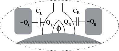
Figure 3: Aharonov-Bohm loop capacitively coupled to external charged gates. The system as a whole (inside the dashed line; this includes the full cavity which we drew only partially) is electrically neutral, which does not prevent charge fluctuations in the arms of the loop to occur, provided they are compensated by fluctuations in the gates. The fluctuations in $Q_{\rm L}$ and $Q_{\rm R}$ induce fluctuations of the internal electric potential in the corresponding arm.

Following Ref. see01 , we consider that our system as a whole, including charged gates defining the cavity and the Aharonov-Bohm ring, is electrically neutral, as sketched in Fig. 3. This does not prevent local charge fluctuations to occur, which in their turn induce fluctuations of the electric potential felt by the electrons. This is a specific example of dephasing induced by an external source, in this case the electric charges on the gates defining the system, which must fluctuate to ensure that the fluctuations inside the circuit are compensated to make the whole system electrically neutral. These fluctuations result in dephasing, and without loss of generality, we will assume that they affect only electrons passing through one, say the left intermediate lead, during the traversal time $\tau_{\rm L}=L_{\rm L}/v$ through that lead.

We consider the case of weak coupling, where the trajectories are unaffected by the coupling to external degrees of freedom. Dephasing is introduced in our calculation via the substitution

$$S_{s}(x,y_{\rm o};{\bf r}_{0};t)\rightarrow S_{s}(x,y_{\rm o};{\bf r}_{0};t)+\int_{0}^{\tau_{\rm L}}dt\;\varphi_{s}(t).$$ (21)

Here $\varphi_{s}(t)$ gives the additional action phase accumulated by an electron traveling on path $s$ and interacting with the dephasing source at time $t$.

Using the central limit theorem, Eqs. (12) and (20) have then to be multiplied by

$$\exp[-\int_{0}^{\tau_{L}}dt_{1}\int_{0}^{\tau_{L}}dt_{2}\langle\varphi_{s}(t_{1})\varphi_{s}(t_{2})\rangle_{s}/2],$$ (22)

where $\langle...\rangle_{s}$ denotes an average over the distribution of phases on different classical trajectories. Further assuming an exponential decay of the phase correlator $\langle\varphi_{s}(t_{1})\varphi_{s}(t_{2})\rangle_{s}=\langle\varphi_{s}^{2}(0)\rangle_{s}\exp[-|t_{1}-t_{2}|/\tau_{c}]$, one gets, in the limit $\tau_{c}\ll\tau_{\rm L}$, an exponential suppression of the flux response

$$\langle g^{2}(\phi)\rangle = \frac{N_{\rm B}\;N_{\rm T}}{(N_{\rm B}+N_{\rm T})^{2}}\cos^{2}(2\pi\phi/\phi_{0})e^{-\tau_{\rm L}/\tau_{\varphi}},$$ (23)

where $\tau_{\varphi}^{-1}=2\tau_{c}\langle\varphi_{s}^{2}(0)\rangle_{s}$. In the limit of Nyquist noise, a self-consistent calculation of the phase correlator has been performed in Ref. see01 , within the one-potential approximation, i.e. assuming that the fluctuations of the electric potential are spatially homogeneous inside one arm. A linear temperature dependence of the dephasing rate was obtained, which in our case translates into

$$\tau_{\varphi}^{-1}=2\tau_{c}\langle\varphi_{s}^{2}(0)\rangle_{s}=8\pi\gamma^{2}_{\rm L}k_{B}T/N_{\rm L}.$$ (24)

Here, $\gamma_{\rm L}\leq 1$ stands for the ratio between the electrochemical and the electrical capacitance of the left arm see01 . In the weak coupling limit we are considering, one has $\gamma_{\rm L}\simeq 1$. Both the exponential damping of the Aharonov-Bohm flux and the linear temperature dependence of the dephasing rate are in agreement with the experimental results of Ref. han01 on Aharonov-Bohm conductance oscillations in few-channel ballistic systems. Our results (22)-(24) extend those of Ref. see01 to the many-channel case.

As a side remark, we note that in the other limit $\tau_{c}\gg\tau_{\rm L}$, one gets a Gaussian suppression of the flux response in the traversal time $\tau_{\rm L}$,

$$\langle g^{2}(\phi)\rangle = \frac{N_{\rm B}\;N_{\rm T}}{(N_{\rm B}+N_{\rm T})^{2}}\cos^{2}(2\pi\phi/\phi_{0})e^{-\tau^{2}_{\rm L}/\tau_{\varphi}\tau_{c}},$$ (25)

with the same dephasing time as above. This Gaussian damping has not been obtained previously. Indeed, previous works always assumed $\delta$-correlated phases, $\langle\varphi_{s}(t_{1})\varphi_{s}(t_{2})\rangle_{s}\propto\delta(t_{1}-t_{2})$, meaning $\tau_{c}/\tau_{\rm L}\rightarrow 0$.

To close this chapter, we remark that the same dephasing behavior will occur in regular systems as long as the phase correlator decay fast enough. While in that case, an exponential decay is not at all obvious from a dynamical point of view, we stress that, in the limit of long traversal times $\tau_{\rm L}\gg\tau_{c}$, the minimal requirement for an exponential damping as in Eq. (23) is a power law decay of the phase correlator $\langle\varphi(t_{1})\varphi(t_{2})\rangle=\langle\varphi(0)\varphi(0)\rangle[\tau_{c}/(\tau_{c}+|t_{1}-t_{2}|)]^{\alpha}$ with $\alpha>1$.

V Conclusion

We have presented a semiclassical calculation of the flux dependence of the probability current and the conductance in two distinct Aharonov-Bohm set-ups (see Fig. 2). We have shown how the interference fringes in the probability current disappear in chaotic systems in the case of cavities with large dwell times, whereas they may persist in the case of a regular cavity. This is in agreement with and sheds light on the numerical results of Ref. casati04 . Simultaneously, we showed how the situation is completely different in the transport set-up, where the flux response of the conductance becomes universal in the chaotic case. This universality is lost in the case of integrable cavities, where we conjectured that the flux response may be of the same order as the conductance itself.

In the transport set-up, we argued that dephasing from external degrees of freedom is necessary to wash out the flux-periodic interference fringes in the conductance. We introduced dephasing in a similar way as in Refs. see03 ; see01 and found that flux-dependent interference fringes in the conductance vanish exponentially, $\exp[-\tau_{\rm L}/\tau_{\varphi}]$. Both this exponential damping and the linear temperature-dependence of the dephasing time (24) are in agreement with transport experiments on ballistic Aharonov-Bohm systems han01 . Our results confirm the standard view that external sources of decoherence are generally required to induce a complete quantum–classical correspondence.

Our semiclassical treatment extends the results of Refs. see03 ; see01 to the many-channel case. Still, the dephasing behavior of Eqs. (22)-(23) relies on the one-potential approximation giving the linear temperature dependence of the phase correlator, Eq. (24). Because Ref. casati04 considered the other limit of sub-wavelength slits, it is likely that diffraction effects play a role there that was neglected here. However, we do not expect diffraction to alter the situation qualitatively.

One of our motivations was to reconcile the results of Ref. casati04 with well-known mesoscopic physics theoretical and experimental results. That is why we deliberately made the hypothesis of forward scattering only, that particles entering one of the intermediate leads (indicated by $L$ and $R$ in Fig. 2) are transferred to the outgoing lead with probability one. This is justified in the case where that latter lead is somehow wider than the two intermediate leads together, $N_{\rm T}\gtrsim N_{\rm R}+N_{\rm L}$. It would be interesting to lift that hypothesis, and consider the emergence of higher flux harmonics and of flux-dependent weak localization corrections to the average conductance, and the influence that dephasing has on them. We expect that the presence of weak-localization corrections would result in the usual Lorentzian damping of the amplitude of Aharonov-Bohm interference fringes in the disorder-averaged conductance (as opposed to the typical conductance calculated here). Further investigations are however necessary to confirm this.

References

- (1) Quantum Theory and Quantum Measurement, J.A. Wheeler and W.H. Zurek Eds., Princeton University Press (1983).
- (2) G.P. Berman and G.M. Zaslavsky, Physica A 91, 450 (1978).
- (3) B.L. Altshuler, A.G. Aronov, and D. Khmelnitskii, J. Phys. C 15, 7367 (1982).
- (4) E. Joos and H.D. Zeh, Z. für Physik B 59, 223 (1985).
- (5) A.O. Caldeira and A.J. Leggett, Phys. Rev. A 31, 1059 (1985).
- (6) M. Büttiker, Phys. Rev. B 33, 3020 (1986).
- (7) G. Casati and B.V. Chirikov, Physica D 86, 220 (1995).
- (8) G. Casati and T. Prosen, nlin.CD/0403038.
- (9) Y. Imry, Introduction to Mesoscopic Physics (Oxford, 1997); E. Akkermans and G. Montambaux, Physique Mésoscopique des Electrons et des Photons (EDP Sciences, 2004).
- (10) A.G. Aronov and Yu.V. Sharvin, Rev. Mod. Phys. 59, 755 (1987).
- (11) R.A. Webb, S. Washburn, C.P. Umbach, and R.B. Laibowitz, Phys. Rev. Lett. 54, 2696 (1985).
- (12) A. Yacoby, M. Heiblum, D. Mahalu and H. Shtrikman, Phys. Rev. Lett. 74, 4047 (1995).
- (13) H.-F. Cheung, E.K. Riedel, and Y. Gefen, Phys. Rev. Lett. 62, 587 (1989).
- (14) F. von Oppen and E.K. Riedel, Phys. Rev. Lett. 66, 84 (1991); B.L. Altshuler, Y. Gefen, and Y. Imry, Phys. Rev. Lett. 66, 88 (1991).
- (15) L.P. Lévy, G. Dolan, J. Dunsmuir, and H. Bouchiat, Phys. Rev. Lett. 64, 2074 (1990); V. Chandrasekhar, R.A. Webb, M.J. Brady, M.B. Ketchen, W.J. Galagher, and A. Kleinsasser, Phys. Rev. Lett. 67, 3578 (1991).
- (16) G. Seelig, S. Pilgram, and M. Büttiker, Turk. J. of Phys. 27, 331 (2003).
- (17) T. Ludwig and A.D. Mirlin, Phys. Rev. B 69, 193306 (2004); C. Texier and G. Montambaux, cond-mat/0505199.
- (18) S. Kawabata and K. Nakamura, J. Phys. Soc. Jpn 65, 3708 (1996); Phys. Rev. B 57, 6282 (1998).
- (19) W. Bauer and G.F. Bertsch, Phys. Rev. Lett. 65, 2213 (1990).
- (20) H.U. Baranger, R.A. Jalabert, and A.D. Stone, Phys. Rev. Lett. 70, 3876 (1993); K. Richter and M. Sieber, Phys. Rev. Lett. 89, 206801 (2002).
- (21) R. Landauer, Phil. Mag. 21, 863 (1970); M. Büttiker, Phys. Rev. Lett. 57, 1761 (1986).
- (22) F. von Oppen and E.K. Riedel, Phys. Rev. B 48, 9170(R) (1993).
- (23) G. Seelig and M. Büttiker, Phys. Rev. B 64, 245313 (2001).
- (24) A.E. Hansen, A. Kristensen, S. Pedersen, C.B. Sørensen, and P.E. Lindelof , Phys. Rev. B 64, 045327 (2001); K. Kobayashi, H. Aikawa, S. Katsumoto, and Y. Iye, J. Phys. Soc. Jpn. 71, 2094 (2002).