The implications of resonant x-ray scattering data on the physics of the insulating phase of V₂O₃.

Abstract

We have performed a quantitative analysis of recent resonant x-ray scattering experiments carried out in the antiferromagnetic phase of V₂O₃ by means of numerical ab-initio simulations. In order to treat magnetic effects, we have developed a method based on multiple scattering theory (MST) and a relativistic extension of the Schrödinger Equation, thereby working with the usual non relativistic set of quantum numbers $l,m,\sigma$ for angular and spin momenta. Electric dipole-dipole (E1-E1), dipole-quadrupole (E1-E2) and quadrupole-quadrupole (E2-E2) transition were considered altogether. We obtain satisfactory agreement with experiments, both in energy and azimuthal scans. All the main features of the V K edge Bragg-forbidden reflections with $h+k+l=$odd can be interpreted in terms of the antiferromagnetic ordering only, ie, they are of magnetic origin. In particular the ab-initio simulation of the energy scan around the (1,1,1)-monoclinic reflection excludes the possibility of any symmetry reduction due to a time-reversal breaking induced by orbital ordering.

I Introduction

In the last fifteen years, after the discovery of high-temperature superconductivity in cuprates, there has been an upsurge of renewed interest in the electronic properties of transition metal oxides.[1] Among the different techniques applied to investigate such materials, resonant x-ray scattering (RXS) has proved to be a powerful tool to extract direct informations about magnetic[2, 3] and electronic [4, 5] distributions: no other methods have the same flexibility to detect lattice, orbital and magnetic anisotropies within the same experimental setup.[6] Yet, a general theoretical comprehension of some important implications of this technique is still lacking, and this circumstance has sometimes led to incorrect conclusions about the origin of the anomalous signals.[7, 8, 9] This is particularly true for magnetic RXS, where the absence of numerical ab-initio simulations has strongly limited the possibility of quantitative investigations. Only recently few papers have appeared dealing with this matter. In particular Takahashi et al.[11] have used the ab initio local density approximation (LDA) + $U$ scheme, taking also into account spin-orbit interaction, to describe such phenomena. In this way they were able to calculate the magnetic RXS in the energy region of the $4p$ conduction band in KCuF₃.

One of the purposes of this paper is to present an alternative method to deal with magnetic phenomena, which we believe physically more intuitive, based on a relativistic extension of the Schrödinger Equation and the multiple scattering theory (MST). This extension is obtained by eliminating the small component of the relativistic wave-function in the Dirac Equation and working only with the upper component,[12] thereby using the more intuitive non relativistic set of quantum numbers $(l,m,\sigma)$ for the angular and spin momenta. In order to take into account spin-polarized potentials and spin-orbit interaction in the framework of MST we solve a two-channel problem, in each atomic sphere, for the two spin components of the wave-function coupled by the spin-orbit interaction. The condition $m+\sigma=m^{\prime}+\sigma^{\prime}$ must be satisfied, due to the local conservation of the $z$-projection of total angular momentum $\vec{j}=\vec{l}+\vec{\sigma}$. We have implemented the computer code to calculate magnetic RXS into the FDMNES package.[13, 14]

Secondly and more important, we present here the first application of this method to deal with the case of V₂O₃, which has attracted considerable attention in the past four years, [8, 9, 15, 16, 17, 18, 19, 20, 21] due to the peculiar interplay of magnetic and orbital ordering. By performing a quantitative analysis of the recent RXS experiments carried out by Paolasini et al.[16, 17] at the vanadium K edge, we shall try to establish the magnetic space group of the monoclinic phase, in the endeavor to resolve some controversies that are still going on in the scientific community.

A brief history of the most recent findings about V₂O₃ will motivate our work. This compound is a Mott-Hubbard system showing a metal-insulator transition at around 150 K from a paramagnetic metallic (PM) to an anti-ferromagnetic insulating (AFI) phase due to the interplay between band formation and electron Coulomb correlation.[22] A structural phase transition takes place, at the same temperature, from corundum to monoclinic crystal class. In recent years, on the basis of an old theoretical model by Castellani et al.,[23] Fabrizio et al.[15] suggested that a direct observation of orbital ordering (OO) could have been possible by means of RXS. Soon after Paolasini et al.[16] interpreted the forbidden (111) monoclinic Bragg-forbidden reflection as an evidence of such OO. All this gave rise to an intense debate [8, 9, 17, 18, 19, 20, 21] whose main achievement was to prove the incorrectness of the old Castellani et al. model. In fact, non-resonant x-ray magnetic scattering experiments [16] and absorption linear dichroism[24] showed that the atomic spin on vanadium ions is S=1, and not S=1/2, as supposed in Ref. [[23]]. Yet, none of the attempts to explain the origin of the (111) monoclinic reflection[8, 9, 17, 18, 19, 20] can be considered satisfactory, for reasons that will be clearer in the following. Here we just recall that many different physical mechanisms have been proposed, from the antiferro-quadrupolar ordering of the 3$d$ orbitals, [8] to the combined action of the ordered orbital and magnetic degrees of freedom;[9] from an orbital ordering associated with a reduction of the magnetic symmetry,[18] to the anisotropies in the magnetic octupolar[19] or toroidal distribution.[20]

In this paper we shall focus on a series of Bragg-forbidden reflections measured by Paolasini and collaborators.[16, 17] Of particular interest, from a theoretical point of view, is the set of data of Ref. [[17]], where the different reflections have been collected with particular care on their relative intensities, and energy and azimuthal scans have been performed in both the rotated ($\sigma\pi$) and unrotated ($\sigma\sigma$) channels. Thanks to the wide information content of these data, we are able to demonstrate that the signal cannot be due to any kind of orbital ordering or charge anisotropy and it must be magnetic. Moreover we can show that both mechanisms suggested in Refs. [[19, 20]] can be at work for the (1,1,1) reflection, as there is no extinction rule for either dipole-quadrupole or quadrupole-quadrupole transitions. Which of the two contributions dominates depends strongly on the kind of reflection and on the azimuthal angle. To reach this conclusion ab initio calculations have proved necessary.

The next section is devoted to the description of our method to deal with magnetic phenomena without resorting to the Dirac equation. We shall work in the framework of MST with muffin-tin approximation or within the finite difference method (FDM),[13] ie, without approximation on the geometrical shape of the potential. In Sec. III we introduce the crystal and electronic properties of V₂O₃ and compare our results with the experimental data, discussing the physical mechanism behind each reflection. Finally we draw some conclusions on the possibility of gaining information about orbital and magnetic degrees of freedom by means of RXS.

II Method of calculation

A RXS and related spectroscopies

Core resonant spectroscopies are described by the virtual processes that promote a core electron to some empty energy levels. They all depend on the transition matrix elements of the operator $\hat{O}$ expressing the interaction of electromagnetic radiation with matter:

$$M_{ng}=\langle\psi_{n}|\hat{O}|\psi_{g}\rangle$$ (1)

Here $\psi_{g}$ is the ground state and $\psi_{n}$ the photo-excited state. In the x-ray regime, the operator $\hat{O}$ is usually written through the multipolar expansion of the photon field up to the electric quadrupole term[25]:

$$\hat{O}^{i(o)}=\vec{\epsilon}^{i(o)}\cdot\vec{r}~{}\big{(}1-\frac{1}{2}i\vec{k}^{i(o)}\cdot\vec{r}\big{)}$$ (2)

where $\vec{r}$ is the electron position measured from the absorbing ion, $\vec{\epsilon}^{i(o)}$ is the polarization of the incoming (outgoing) photon and $\vec{k}^{i(o)}$ its corresponding wave vector. In the following dipole and quadrupole will refer to electric dipole and electric quadrupole. In RXS the global process of photon absorption, virtual excitation of the photoelectron, and subsequent decay with re-emission of a photon, is coherent throughout the crystal. Such a coherence gives rise to the usual Bragg diffraction condition, that can be expressed, at resonance, as:

$$F=\sum_{a}e^{i\vec{Q}\cdot\vec{R}_{a}}(f_{0a}+f_{a}^{\prime}+if_{a}^{\prime\prime})$$ (3)

where $\vec{R}_{a}$ stands for the position of the scattering ion $a$, $\vec{Q}$ is the diffraction vector and $f_{0}$ is the usual Thomson factor. The resonant part, $f^{\prime}+if^{\prime\prime}$, is the anomalous atomic scattering factor (ASF), given by the expression[26]:

$$f^{\prime}+if^{\prime\prime}=\frac{m_{e}}{\hbar^{2}}\frac{1}{\hbar\omega}\sum_{n}\frac{(E_{n}-E_{g})^{3}M_{ng}^{o*}M_{ng}^{i}}{\hbar\omega-(E_{n}-E_{g})-i\frac{\Gamma_{n}}{2}}$$ (4)

Here $\hbar\omega$ is the photon energy, $m_{e}$ the electron mass, $E_{g}$ the ground state energy, and $E_{n}$ and $\Gamma_{n}$ are the energy and inverse lifetime of the excited states. In practice, the intermediate states $\psi_{n}$ are in the continuum, normalized to one state per Rydberg. For this reason it is useful to label them by their energy $E$ and re-express Eq. (4) as:

$$f^{\prime}+if^{\prime\prime}=-m_{e}\omega^{2}\sum_{n}\int_{E_{F}}^{\infty}\frac{{M}_{ng}^{o*}{M}_{ng}^{i}}{E-E_{g}-\hbar\omega-i\frac{\Gamma(E)}{2}}dE$$ (5)

using the fact that, at resonance, $E_{n}-E_{g}\simeq\hbar\omega$. $E_{F}$ is the Fermi energy. In Eq. (5) the summation over $n$ is now limited to states having the energy $E$.

It is now straightforward to make the connection with another spectroscopic technique: x-ray near edge absorption (XANES). In this case the cross-section simply corresponds to the imaginary part of the ASF when $\hat{O}_{o}=\hat{O}_{i}$ (forward scattering). Choosing prefactors in order to have $f^{\prime\prime}$ in units of the classical electron radius, $r_{0}\simeq 2.82\cdot 10^{-15}$ m, and the absorption cross section $\sigma$ in megabarn, we have the relation:

$$\sigma=-4\pi~{}10^{22}~{}\frac{a_{0}^{2}\alpha^{3}m_{e}c^{2}}{\hbar\omega}f^{\prime\prime}$$ (6)

where $a_{0}$ is the Bohr radius, $\alpha$ is the fine structure constant and $c$ is the speed of light. The close connection between the two spectroscopies is thus evident.

The use of RXS can have some advantages in exploring electronic properties compared to the absorption techniques. First, with RXS it is possible to select different relative conditions in incoming and outgoing polarizations and wave vectors, and this gives more opportunities to probe the magnetic and electronic anisotropies of the material. Secondly, RXS can be more site selective than XANES, due to the Bragg factor (3). For instance, it is possible, in magnetite, to be sensitive only to octahedral Fe³⁺-sites and not to tetrahedral Fe^3.5+-sites [27] or, in manganites, to probe only Mn³⁺-ions and not Mn⁴⁺-ions.[28] This can be achieved at reflections that are Bragg-forbidden off-resonance, but become detectable, in resonant conditions, because of non-symmorphic symmetry elements (glide planes, screw axes) in the crystal space group.[29] In these cases the Thomson factors $f_{0}$ (Eq. 3) drop out and one is just sensitive to the changes of the ASF (Eq. (4)) that depend on the relative electronic and magnetic anisotropies on the ions related by such non-symmorphic symmetry elements. It is indeed in such kinds of reflections that orbital ordering or magnetic scattering were reported and they will be the main subject of the present study.

B Cartesian Tensor approach

In Sec. III we shall deal with the symmetry operations of the crystal space group of V₂O₃, in order to evaluate the structure factor for RXS. Because of this, it is very useful to write explicitly the dipole and quadrupole components of the matrix elements in Eq. (5). Remembering that incoming and outgoing x-rays can have different polarizations and wave vectors, we get:

$$\sum_{n}{M}_{ng}^{o*}{M}_{ng}^{i} = \sum_{\alpha\beta}\epsilon_{\alpha}^{o*}\epsilon_{\beta}^{i}D_{\alpha\beta}$$ (7)

$$- \frac{i}{2}\sum_{\alpha\beta\gamma}\epsilon_{\alpha}^{o*}\epsilon_{\beta}^{i}(k_{\gamma}^{i}I_{\alpha\beta\gamma}-k_{\gamma}^{o}I_{\beta\alpha\gamma}^{*})$$ (8)

$$+ \frac{1}{4}\sum_{\alpha\beta\gamma\delta}\epsilon_{\alpha}^{o*}\epsilon_{\beta}^{i}k_{\gamma}^{o}k_{\delta}^{i}Q_{\alpha\beta\gamma\delta}$$ (9)

where $\alpha$, $\beta$, $\gamma$ and $\delta$ are cartesian coordinate labels and $D_{\alpha\beta}$, $I_{\alpha\beta\gamma}$ and $Q_{\alpha\beta\gamma\delta}$, the dipole-dipole (dd), dipole-quadrupole (dq) and quadrupole-quadrupole (qq) contributions, respectively. Their explicit expression is given by:

$$D_{\alpha\beta} = \sum_{n}\langle\psi_{g}|r_{\alpha}|\psi_{n}\rangle\langle\psi_{n}|r_{\beta}|\psi_{g}\rangle$$ (10)

$$I_{\alpha\beta\gamma} = \sum_{n}\langle\psi_{g}|r_{\alpha}|\psi_{n}\rangle\langle\psi_{n}|r_{\beta}r_{\gamma}|\psi_{g}\rangle$$ (11)

$$Q_{\alpha\beta\gamma\delta} = \sum_{n}\langle\psi_{g}|r_{\alpha}r_{\beta}|\psi_{n}\rangle\langle\psi_{n}|r_{\gamma}r_{\delta}|\psi_{g}\rangle$$ (12)

Note that at a K-edge, in absence of spin-orbit interaction and time-reversal breaking potentials, $D$, $I$ and $Q$ are all real.

C Calculation of the excited states

The main difficulty in the ab-initio evaluation of the ASF is the determination of the excited states. Two different procedures, MST and FDM, have already been developed for non-magnetic cases, and the corresponding packages[14] used in some XANES[30] and RXS[10, 31] applications. In the following we introduce a relativistic extension of the ab initio cluster approach, for both MST and FDM, that is still mono-electronic but includes the spin-orbit interaction and allows to handle magnetic processes. The importance of the FDM procedure to avoid the muffin-tin approximation has already been reported[13] and will not be detailed here again. Note only that with FDM the intermediate states are calculated by solving the Schrödinger equation without any approximation on the geometrical shape of the potential, ie, we do not need to use, as usually in MST approaches, a spherically averaged potential in the atomic spheres and a constant among them. This point is essential to study orbitally ordered materials, where an anisotropic orbital distribution is the key-feature of the system and no spherically averaged potentials would be adequate for its description. Unfortunately, large cluster calculations with FDM are prohibitively long in computing time and require a lot of computer memory: that’s why, when appropriate, MST is preferred.

In order to treat magnetic effects in MST we have considered the relativistic extension of Schrödinger equation obtained by solving Dirac equation exactly for the upper component of the wave-function, as described by Wood and Boring.[12] This approach ensures that the singularity of the potential at the nuclear center is of centrifugal type ($\sim r^{-2}$) even in the presence of spin-orbit terms (so that the usual fuchsian method of solution can be used). It also allows us to work with the usual non relativistic set of quantum numbers ($l,m,\sigma$) of angular and spin momenta, which we find much more intuitive than the relativistic set. Our one particle basis will therefore comprise spin-orbit coupled core states of the form:

$$\Phi^{c}_{j,j_{z};l_{c}}(\vec{r}) = R_{j}^{c}(r)|j,j_{z};l_{c})$$ (13)

$$= R_{j}^{c}(r)\sum_{m_{c}\sigma}Y_{l_{c}m_{c}}\chi_{\sigma}\left(l_{c}m_{c}1/2\sigma|j,j_{z}\right)$$ (14)

and valence excited states which are multiple scattering solutions of the Schrödinger equation with spin-polarized potentials. In atomic units:

$$\left\{\bigtriangledown^{2}+k_{e}^{2}-V_{0}(\vec{r})-V_{1}(\vec{r})s_{z}-2V_{2}(\vec{r})\vec{\ell}\cdot\vec{s}\right\}\Psi_{\vec{k}_{e},s}(\vec{r})=0$$

(15)

These latters are supplemented by the scattered wave boundary conditions:

$$\Psi_{\vec{k}_{e},s}(\vec{r})=e^{i\vec{k}_{e}\cdot\vec{r}}\chi_{s}-f(\vec{k}_{e},s;\vec{r},s^{\prime})\frac{e^{k_{e}r}}{r}\chi_{s^{\prime}}$$ (16)

In Eq. (13) $\left(l_{c}m_{c}1/2\sigma|j,j_{z}\right)$ are the Clebsch-Gordan coefficients. In Eq. (15) $V_{0}(\vec{r})$ is the average of spin up and spin down potentials, $V_{1}(\vec{r})$ their difference and $V_{2}(\vec{r})$ the usual spin-orbit term. Such potentials already embody the relativistic corrections due to the reduction of the upper Dirac component of the wave function to an effective Schrödinger equation.[12]

In the muffin-tin approximation the solution inside the i-th atomic muffin-tin sphere can be written as:

$$\Psi_{\vec{k}_{e},s}(\vec{r}_{i})=\sum_{l}\sum_{m\sigma}\sum_{m^{\prime}\sigma^{\prime}}R_{lm\sigma}^{lm^{\prime}\sigma^{\prime}}(r_{i})B^{i}_{lm^{\prime}\sigma^{\prime}}(\vec{k}_{e},s)Y_{lm}(\hat{{r}}_{i})\chi_{\sigma}$$

(17)

where at the muffin-tin radius $\rho_{i}$ the radial functions $R_{lm\sigma}^{lm^{\prime}\sigma^{\prime}}(r_{i})$ match smoothly to the following combination of Bessel and Hankel functions via the atomic $t_{lm\sigma,lm^{\prime}\sigma^{\prime}}$ matrices (defined below):

$$R_{lm\sigma}^{lm^{\prime}\sigma^{\prime}}(\rho_{i})=j_{l}(k\rho_{i})t^{-1}_{lm\sigma,lm^{\prime}\sigma^{\prime}}-i\delta_{lm\sigma,lm^{\prime}\sigma^{\prime}}h_{l}^{+}(k\rho_{i})$$ (18)

With a proper normalization of these radial functions to one state per Rydberg, the scattering amplitudes $B^{i}_{L\sigma}(\vec{k}_{e},s)$ obey the equations (writing $L$ for $lm$):

$$\sum_{j}\sum_{L^{\prime}\sigma^{\prime}}M^{ij}_{L\sigma,L^{\prime}\sigma^{\prime}}B^{j}_{L^{\prime}\sigma^{\prime}}(\vec{k}_{e},s)=\delta_{s\sigma}i^{l}Y_{L}(\hat{{k}}_{e})e^{i\vec{k}_{e}\cdot\vec{R}_{i}}$$

where

$$M^{ij}_{L\sigma,L^{\prime}\sigma^{\prime}}=\left(t^{-1}_{lm\sigma,l^{\prime}m^{\prime}\sigma^{\prime}}\delta_{ij}\delta_{ll^{\prime}}\delta_{m+\sigma,m^{\prime}+\sigma^{\prime}}+G^{ij}_{L,L^{\prime}}\delta_{\sigma,\sigma^{\prime}}\right)$$

is the usual multiple scattering matrix, generalized to spin variables, and $\vec{R}_{i}$ denotes the position of the i-th atom in the cluster with respect to the origin of the coordinates. The atomic $t$-matrix $t_{lm\sigma,lm^{\prime}\sigma^{\prime}}$ describes the scattering amplitude of an electron impinging the atomic potential with angular momentum $l$, azimuthal component $m$ and spin $\sigma$ into a state with quantum numbers $l,m^{\prime},\sigma^{\prime}$. The conservation of the total angular momentum $\vec{j}=\vec{l}+\vec{s}$ and its $z$-projection implies the constraint $m+\sigma=m^{\prime}+\sigma^{\prime}$. Note that also $l$ is unchanged in the scattering process, since in the muffin-tin approximation the potential has spherical symmetry.

By introducing as usual[33] the scattering path operator $\tau^{ij}_{L\sigma,L^{\prime}\sigma^{\prime}}$ as the inverse of $M^{ij}_{L\sigma,L^{\prime}\sigma^{\prime}}$, the solution for the scattering amplitudes $B^{i}_{L\sigma}$ is given by:

$$B^{i}_{L\sigma}(\vec{k}_{e},s)=\delta_{\sigma s}\sum_{j}\sum_{L^{\prime}}\tau^{ij}_{L\sigma,L^{\prime}s}i^{l^{\prime}}Y_{L^{\prime}}(\hat{{k}}_{e})e^{i\vec{k}_{e}\cdot\vec{R}_{j}}$$ (19)

The scattering path operator $\tau^{ij}_{L\sigma,L^{\prime}\sigma^{\prime}}$ represents the probability amplitude for the excited photoelectron to propagate from site $i$, with angular momentum $L$ and spin $\sigma$, to site $j$ with angular momentum $L^{\prime}$ and spin $\sigma^{\prime}$. It is the obvious generalization of the corresponding spin-independent quantity.[33]

We now have all the ingredients to perform the intermediate sum in Eq. (5). Using the expression given Eq. (17) for the state $|\psi_{n}\rangle$ in the matrix elements of the numerator, the sum over $n$ becomes an integral over the escape direction of the photoelectron, $\hat{k}_{e}$, at fixed energy, $E=k_{e}^{2}$. When we perform the integral over the energy, we get the product of two smoothly varying radial matrix elements of the type $\langle R_{lm\sigma}^{lm^{\prime}\sigma^{\prime}}(r)|r^{\nu}|R_{j}^{c}(r)\rangle$ times the appropriate angular (Gaunt) coefficient. The exponent ${\nu}$ is determined by the polar order of the transition. This is further multiplied by the angular integral of the product of the two scattering amplitudes $B^{i}_{L\sigma}$, $B^{j}_{L^{\prime}\sigma^{\prime}}$ centered on the absorbing sites. This latter can be simplified by the use of a generalized optical theorem[32]:

$$\sum_{s}\int d{\hat{k}}_{e}B^{i}_{L\sigma}(\vec{k}_{e},s)B^{j}_{L^{\prime}\sigma^{\prime}}(\vec{k}_{e},s)=\Im\tau^{ij}_{L\sigma,L^{\prime}\sigma^{\prime}}$$ (20)

As a consequence, the knowledge of $\tau$ at all relevant energies, and of the radial solutions $R_{lm\sigma}^{lm^{\prime}\sigma^{\prime}}(r)$ on the photoabsorber are sufficient to calculate the ASF.

In the case of V₂O₃, in order to construct the spin-polarized atomic potentials, we have used the prescription by von Barth and Hedin[35]: they were derived from the non-self-consistent spin-polarized charge density obtained by superimposing the atomic charge densities with two magnetic electrons on each Vanadium ion, as suggested by the experimental data.[16, 24] We believe that this approximation is not far from reality, as shown a posteriori by the goodness of the results. Given the potential, it is straightforward to calculate the atomic spin dependent $t$-matrix: we just solve the two-channel problem arising from the Schrödinger equation (15) due to the presence of the spin-orbit potential. In this way this latter is treated on the same footing as the other potentials and not in perturbation theory as usually done.

The relativistic extension in the FDM scheme follows closely the previous treatment for MST. The space is partioned, as in the multiple scattering approach, in three regions[14]: i) An outer sphere surrounding the cluster where one impose the scattering behaviour of the wave function given in Eq. (16). ii) An atomic region made up of spheres, around each atom, with radii much smaller than the muffin-tin radii (of the order of 1 a.u. or less). Here the charge density is to a very good approximation spherically symmetric, due to the presence of the core electrons. iii) Finally, an interstitial region where the Laplacian operator of the Schrödinger equation (15) is discretized and the solution is generated on a greed without any approximation on the geometrical shape of the potential. By imposing a smooth continuity of the overall wave function across the boundaries of the three regions, one can determine both the expansion amplitudes of the wave function inside each atom and the scattering T-matrix of the whole cluster in Eq. (16). [13] Note that in this case the spin-orbit potential is not spherically symmetric. We have checked that for a small cluster with close-packed geometry, this approach and the multiple scattering approach with muffin-tin approximation provide almost identical cross sections. Since V₂O₃ is a close-packed structure, if one neglects vanadium voids, we have used MST in the muffin-tin approximation for the magnetic calculations. The FDM scheme was instead used in the calculation of the ASF in the case of orbital ordering.

III The case of V₂O₃

In this section we specialize to the case of V₂O₃, to investigate whether the RXS reflections observed by Paolasini and collaborators [16, 17] are of magnetic or orbital nature. Our result is that magnetic ordering can explain the experimental data with a reasonably good agreement (even if not perfect, for reasons that will be discussed below). On the other hand, we are able to demonstrate that any OO origin of the signal has to be excluded, as it would not fit the energy scan at dipolar energies.

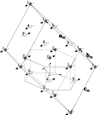
FIG. 1.: Monoclinic cell in the AFI phase of V₂O₃. The numbers label the eight vanadium ions of the unit cell. The arrows show the spin orientations. $a_{m}$, $b_{m}$ and $c_{m}$ are the monoclinic axis. Only V ions are represented: white and gray circles indicate that they are surrounded by differently oriented oxygen octahedra. Two basal planes of the hexagonal corundum cell are also shown.

Next subsection is devoted to the description of the magnetic space group in the AFI phase, as well as the derivation of the anomalous RXS amplitude. In subsection B we analyze the ab-initio calculations for the magnetic RXS, through the procedure previously developed. Finally, in the last part we show that the consequences of a time-reversal breaking OO are not compatible with the experimental data, thus putting a severe constraint on the possible OO theories for V₂O₃.

A Crystal and magnetic structure

As a first step we shall try to establish the magnetic symmetry group in the AFI phase. Our starting point is the crystallographic structure, as given by Dernier and Marezio[36] together with the magnetic data given by Moon[38] and later confirmed by Wei Bao et al. [39]

Referring to the frame and the numbering of vanadium atoms of Fig. 1, we can divide the eight atoms of the monoclinic unit cell into two groups of four, $V_{1},V_{2},V_{3},V_{4}$ and $V_{1^{\prime}}$, $V_{2^{\prime}}$, $V_{3^{\prime}}$, $V_{4^{\prime}}$, with opposite orientations of the magnetic moment. The two groups are related by a body-centered translation. Vanadium-ion magnetic moments, indicated by arrows in the figure, lie perpendicular to the $b_{m}$-axis at an angle of 138⁰ away from the monoclinic $c_{m}$-axis. Neglecting the magnetic moments, the previous two groups of four atoms with their oxygen environments are translationally equivalent.

We can infer from these data that the magnetic space group can be written as $P2/a+{\hat{T}}\{{\hat{E}}|t_{0}\}P2/a$, where ${\hat{T}}$ is the time-reversal operator and $t_{0}$ the body-centered translation. The monoclinic group $P2/a$ contains four symmetry operations: the identity ${\hat{E}}$, the inversion ${\hat{I}}$, the two-fold rotation about the monoclinic $b_{m}$ axis ${\hat{C}}_{2b}$ and the reflection ${\hat{m}}_{b}$ with respect to the plane perpendicular to this axis. All these operations are associated to the appropriate translations, as shown in the following table:

$$\begin{array}[]{c|cccc}{\rm atom}&{\rm position}&{\rm spin}&{\rm sym.}&{\rm translation}\\ \hline\cr V_{1}&(u,v,w)&\uparrow&{\hat{E}}&0\\ V_{2}&(-u,-v,-w)&\uparrow&{\hat{I}}&0\\ V_{3}&(\frac{1}{2}+u,-v,w)&\uparrow&{\hat{T}\hat{m}_{b}}&(\frac{1}{2},0,0)\\ V_{4}&(\frac{1}{2}-u,v,-w)&\uparrow&{\hat{T}\hat{C}_{2b}}&(\frac{1}{2},0,0)\\ V_{1^{\prime}}&(\frac{1}{2}+u,\frac{1}{2}+v,\frac{1}{2}+w)&\downarrow&{\hat{T}}&(\frac{1}{2},\frac{1}{2},\frac{1}{2})\\ V_{2^{\prime}}&(\frac{1}{2}-u,\frac{1}{2}-v,\frac{1}{2}-w)&\downarrow&{\hat{T}\hat{I}}&(\frac{1}{2},\frac{1}{2},\frac{1}{2})\\ V_{3^{\prime}}&(u,\frac{1}{2}-v,\frac{1}{2}+w)&\downarrow&{\hat{m}_{b}}&(0,\frac{1}{2},\frac{1}{2})\\ V_{4^{\prime}}&(-u,\frac{1}{2}+v,\frac{1}{2}-w)&\downarrow&{\hat{C}_{2b}}&(0,\frac{1}{2},\frac{1}{2})\end{array}$$

TABLE I.

Here $u=0.3438,\;v=0.0008,\;w=0.2991$ are the fractional coordinates of the atoms in unit of the monoclinic axis. Notice that it is sufficient to calculate the ASF for atom number 1, since all the others can be deduced by applying the symmetry operation indicated in the fourth column of the table.

In the following, we re-analyze the extinction rules for the different reflections $(h,k,l)$ measured by Paolasini et al. [16, 17] in terms of the crystal tensors in the dd, dq and qq channels (Eq. (12)). All the recorded reflections have the same incoming polarization, $\sigma$ (electric field perpendicular to the diffraction plane), whereas the outgoing polarization is analyzed both in the $\sigma$ and $\pi$ channels (this latter with the electric field in the diffraction plane). The azimuthal scans are then registered by rotating the sample around the diffraction vector. We refer to Paolasini et al. [[17]] for the definition of the azimuthal origin: the situation where the scattering plane contains $a$ and $c$ hexagonal axes corresponds to an azimuthal angle of 90 degrees.

From equation (3) and Table I, neglecting the very small component of $\vec{R}$ along $b_{m}$, ($v=0.0008$), we get for each reflection $(h,k,l)$ the expression:

$${\cal F}^{hkl}=(1+(-)^{h}\hat{T}\hat{m_{b}})(e^{i\phi_{hkl}}+e^{-i\phi_{hkl}}\hat{I})$$ (22)

$$(1+(-)^{h+k+l}\hat{T})f_{1}$$ (23)

where $R\simeq(u,0,w)$ is the position of the $V_{1}$ atom, $\phi_{hkl}\equiv\vec{Q}\cdot\vec{R}\equiv 2\pi(hu+lw)$ and $f_{1}$ stands for the ASF as defined in (Eq. 5). Note that $f_{1}$ is a scalar and we adopt the convention, when we say that a symmetry operator acts on $f_{1}$, that it acts only on the tensor components (dd, dq and qq) given by Eq. (12). Focusing on the reflections with $h+k+l=$odd and noticing that $D_{\alpha\beta}$ and $Q_{\alpha\beta\gamma\delta}$ are inversion-even, while $I_{\alpha\beta\gamma}$ is inversion-odd, we find that only the following tensor components contribute to the signal:

$${\cal D}_{\alpha\beta}^{hkl}=4i(1+(-1)^{h+n_{y}+1})\cos(\phi_{hkl})\Im(D_{\alpha\beta})$$ (24)

$${\cal I}_{\alpha\beta\gamma}^{hkl}=4(1+(-1)^{h+n_{y}+1})\sin(\phi_{hkl})\Im(I_{\alpha\beta\gamma})$$ (25)

$${\cal Q}_{\alpha\beta\gamma\delta}^{hkl}=4i(1+(-1)^{h+n_{y}+1})\cos(\phi_{hkl})\Im(Q_{\alpha\beta\gamma\delta})$$ (26)

where $n_{y}$ is the number of $y$ labels among the tensor indices $\alpha$, $\beta$, $\gamma$, and $\delta$. Thus, in order to have a signal, $h$ and $n_{y}$ must have different parity. Notice that all the quantities in Eq. (26) are magnetic, as only imaginary parts of cartesian tensors are involved. Moreover, the three scattering amplitudes are all purely imaginary, as the dq polarizations carry an extra imaginary unit (see Eq. 9). As a consequence, they all interfere. A separate analysis of the three tensors of Eq. (26) gives the following indications.

In the case of dd tensors, when $h$ is odd, the only non-zero component is ${\cal D}_{xz}^{hkl}-{\cal D}_{zx}^{hkl}\propto\langle L_{y}\rangle$. [37] When $h$ is even the non-zero components are ${\cal D}_{xy}^{hkl}-{\cal D}_{yx}^{hkl}\propto\langle L_{z}\rangle$ and ${\cal D}_{yz}^{hkl}-{\cal D}_{zy}^{hkl}\propto\langle L_{x}\rangle$. As the magnetic moment direction is perpendicular to the $b_{m}$-axis, $\langle L_{y}\rangle$ is zero. Thus for odd $h$ no signal is expected in the dipolar region. On the contrary, when $h$ is even, a dd contribution is present. Of course, no $\sigma\sigma$ magnetic scattering is allowed.[26] These facts explain why the experimental spectrum for the $(2,\bar{2},1)_{\sigma\pi}$ shows structures at the $4p$ edge, contrary to the $(2,\bar{2},1)_{\sigma\sigma}$ reflection and to the $(1,1,1)$ and $(3,\bar{1},1)$ reflections for both polarization conditions. Notice that these results had been already derived with similar methods. [18, 19, 20]

These remarks do not apply for qq and dq tensors. They always contribute, for all the investigated reflections, in both $\sigma\sigma$ and $\sigma\pi$ channels, except at some very specific azimuthal angles. At the K edge these tensors measure the transitions to the states with pure 3$d$ or hybridized $3d$-$4p$ character. For this reason they have a finite value just close to the Fermi energy. The physical quantities measured by these operators can be identified as the octupolar magnetic moment for the qq term and the toroidal or quadrupolar magnetic moment for the dq tensor.

B Analysis of the magnetic signal

In order to get the absolute intensities and shape of the spectra, we need now to resort to ab initio calculations. We performed such calculations for the crystal and magnetic structures given in Table I. Thus, we do not neglect the small $v$ value but we shall see that the conclusion given in the previous subsection is not modified. The potential is calculated using a superposition of atomic densities obtained from an atomic, self-consistent Hartree-Fock calculation, with a $3d^{2}$, spin 1, configuration. The MST approach is used with different cluster radii from 3.0 up to 7.2 Å, ie, from a $VO_{6}$ molecule to a cluster containing 153 atoms.

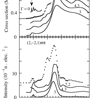
FIG. 2.: Comparison of the experimental (dots) and calculated (continuous line) spectra for the XANES and the $(2,\bar{2},1)_{\sigma\pi}$ reflection at the vanadium K edge. Calculations are performed with three different cluster radii (3, 4.3 and 7.2 Å). The pre-edge feature is also shown before the convolution for the 4.3 Å case. The first structure, indicated by an arrow, is at the energy where the 3d feature of the Bragg peaks appears.

We find that, in order to get the shoulder at 5475 eV in both XANES and $(2,\bar{2},1)_{\sigma\pi}$ spectra, as well as the 5487 eV shoulder in the $(2,\bar{2},1)_{\sigma\pi}$, we need the biggest cluster radius (7.2 Å - see Fig. 2). Nevertheless the main features are present for all Bragg peaks even for the $VO_{6}$ molecule calculation.

The behaviour of the azimuthal scans against the cluster radius looks more complex. The agreement improves up to the 4.3 Å, corresponding to 33 atoms, and then decreases when the cluster radius is further increased. The reason for this is discussed below. For the moment we keep the 4.3 Å radius and compare such energy and azimuthal spectra with the experimental ones, as shown in Figs. 3 and 4.

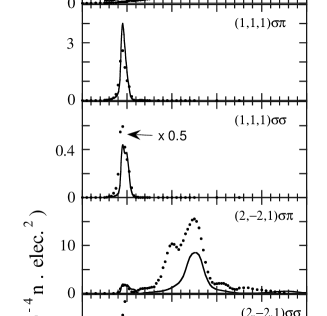
FIG. 3.: Comparison of the experimental (dots) and calculated (continuous line) energy scans for three different reflections. On top is also shown the XANES spectrum. The calculation is performed on a 4.3 Å cluster radius and includes the magnetic ordering. The intensity unit is the electron number squared. Note that the experimental spectra were recorded[17] with a special care on the relative amplitudes. For the $(2,\bar{2},1)$ and $(3,\bar{1},1)$ reflections the azimuthal angle as defined by Paolasini and coworkers is $\psi=15^{0}$. All the mean features are present. An extra scale factor is applied on the experimental dots of the $(1,1,1)_{\sigma\sigma}$ reflection.

Looking at the spectra shown in Fig. 3, we can claim a satisfactory experiment-theory agreement for the different reflections. In particular we get the very thin resonance in the $3d-t_{2g}$ energy range at the $(1,1,1)$ and $(3,\bar{1},1)$ peaks for both $\sigma\sigma$ and $\sigma\pi$ polarization conditions and for the $(2,\bar{2},1)_{\sigma\sigma}$ reflection. The broad intensity in the $4p$ energy range in the $(2,\bar{2},1)_{\sigma\pi}$ is also reproduced.

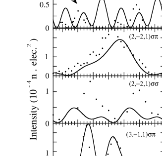
FIG. 4.: Azimuthal scans of the same three reflections shown in Fig. 3. The main features of the experiment (dots) are obtained in the calculation (continuous line). The scans are performed respectively at 5464 eV for the $(1,1,1)$ and $(3,\bar{1},1)$ reflections and 5465 eV for the $(2,\bar{2},1)$. The intensity unit is the number of electrons squared. The azimuth 90⁰ corresponds to the situation where the scattering plane contains the $c$ hexagonal axis.

The intensity ratio between $\sigma\sigma$ and $\sigma\pi$ channels and between the various reflections are also quite good considering the difficulties on both experimental and theoretical sides, even if for the $(1,1,1)_{\sigma\sigma}$ reflection an extra factor improves the agreement with the experiment. Note that, differently from all other reflections, the $(2,\bar{2},1)_{\sigma\pi}$ can contain some non-resonant component not taken into account in our calculation. Moreover, a non-zero offset seems to be present at $(2,\bar{2},1)_{\sigma\sigma}$ on the experimental side, and this is probably responsible for the discrepancy in the corresponding energy and azimuthal scans. The azimuthal scans, shown in Fig. 4, are reasonable for all $\sigma\pi$ reflections. Only the $(1,1,1)_{\sigma\sigma}$ is much less satisfying: yet, the corresponding data belong to the first experiment (Ref. [16], while the others belong to Ref. [17]), and this does not allow to be sure about the relative intensity as in the other cases. Finally, we are also able to reproduce the $\pi$ and $2\pi$ periodicity, expected from the low symmetry of the compound, for the $\sigma\sigma$ and $\sigma\pi$ channels, respectively.

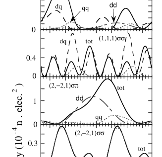
FIG. 5.: Magnetic intensity of the various reflections at the vanadium K edge. The total (continuous line), dd (dash-dotted line), dq (dash line) and qq (dotted line) signals are shown, at the energy E=5465 eV

We judge the agreement between theory and experiment quite satisfactory. Indeed the interference between the dd, dq and qq parts makes the problem really tricky. Foe example, $p$ orbitals are far more delocalized than $d$ ones. For this reason they react in a different way to the core hole screening. In a first approximation $d$ states are more shifted towards lower energy than $p$ states. Thus, the dq terms, which probe the hybridization between $p$ and $d$ orbitals, are strongly influenced by the details of the electronic structure around the photo-absorbing ion. If we consider that V₂O₃ is a strongly correlated electron system, with a quantum-entangled ground-state wave function,[9, 18, 20] we find quite surprising that we have reached such a good agreement in the $3d$ energy region with a one-electron calculation. Our idea is that this can help understanding which features can be explained in terms of an independent particle approach and which cannot (see below). Note that the localization of the $d$ orbitals also explains why the azimuthal scans look better when the calculations are performed using the smaller 4.3 Å cluster radius. To end this discussion we stress that energy spectra profiles around 5464 eV are very sensitive to the azimuthal angle and, vice-versa, azimuthal profiles are very sensitive to the energy. This is due to the fact that qq and dq components have both strong (and different) angular and energy dependence. There are some angles where the calculated profiles appear doubled, with about 1 eV between the two peaks. For instance, this is what happens at the experimental azimuth of the $(3,\bar{1},1)_{\sigma\sigma}$ energy spectrum: a simple shoulder appears at 5465 eV, well described by our calculation.

Finally, we want to comment about the two papers (by Lovesey et al. [19] and by Tanaka.[20]) that have already pointed out the magnetic origin of the $h+k+l=$odd reflections. These works disagree on the physical mechanism of the signal, as for Tanaka only dq terms contribute, while Lovesey and coworkers attribute the signal to a pure qq reflection. Our results on this point show that both dq and qq channels can contribute to the global intensity depending on the reflections (whether $h=$odd or $h=$even) and on the azimuthal angle (see Fig. 5). At the prepeak energy, E=5465 eV, the dq term represents the strongest contribution for the $(1,1,1)$ and $(3,\bar{1},1)$ reflections, even if the qq term is not completely negligeable. For the $(2,\bar{2},1)_{\sigma\sigma}$, on the contrary, the qq contribution is clearly the dominating one. Finally, it is interesting to note that for the $(2,\bar{2},1)_{\sigma\pi}$ reflection the dd term plays the major role even at the $3d$ energies. Anyway the qq contribution has always a non-negligeable influence on the total signal. Comparing our findings with those of Refs. [19, 20] we can state that there are no strict extinction rules regarding dq and qq terms for all these reflections. Nonetheless, the main contribution to $h+k+l=$odd, $h=$odd reflections comes from the dq channel (as in Ref. [20]), while the main term in $h+k+l=$odd, $h=$even reflections is of qq origin (as in Ref. [19]). Such a tensor analysis allows also to identify a feature that is not correclty described by our one-electron calculations, ie, the direction of the magnetic moment. Indeed, a small $L_{y}$ component (about $10\%$ the global moment) is found to contribute to the $h=$odd signal (see Fig. 5), contrary to what expected by our previous theoretical analysis. This result can be explained by noticing that in order to obtain the correct direction of the magnetic moment a molecular, correlated ground-state wave function is needed,[20] which is far beyond the possibilities of our monoelectronic approach.

C Analysis of the ”orbital” signal

In this subsection, we analyze the effect of a time-reversal breaking OO on the signal, in order to determine whether it can affect our previous results. This is not a secondary issue since the original experimental interpretation suggested that the (111)-monoclinic reflection was due to the OO[16] and a big controversy around this point arose in the literature.[8, 9, 18, 20] The reason why we focus on a ”time-reversal breaking” OO is that, for $h+k+l=$odd, the signal is proportional to $({\hat{E}}-{\hat{T}})f_{1}$, as clear from Eq. (23), so that a non-magnetic signal is allowed only when the time-reversal symmetry is broken. This is obtained, for example, when V_i and V${}_{i^{\prime}}$ have a different orbital occupancy,[18] and we call such a situation time-reversal breaking OO. Different types of orbitally-ordered ground states have been suggested in the literature,[9, 18, 23] but none of them possesses such a feature. As a consequence, non-magnetic signals at the (111)_m reflection are not expected, unless some ad hoc hypoteses are made, as recognized in the discussion of Sec. VII.D of Ref. [[18]]. One possible way to get a signal of OO origin is to consider the first excited state found in Ref. [[18]], which has a magnetoelectric (ME) symmetry. It is very close to the ground state ($\simeq 1$ meV) and, because of this, it could be partly occupied. Independently of this, if we consider the two maximal ME subgroups of the full space groups, ie, P2’/a (with symmetry elements ${\hat{E}}$, ${\hat{T}\hat{I}}$, ${\hat{T}\hat{C}_{2b}}$, ${\hat{m}_{b}}$) and P2/a’ (with symmetry elements ${\hat{E}}$, ${\hat{T}\hat{I}}$, ${\hat{C}_{2b}}$, ${\hat{T}\hat{m}_{b}}$), it is in principle possible to get a non-magnetic signal at the (111)_m reflection. In fact, in both cases there are two subgroups of four ions whose electronic densities have anisotropies not connected by time-reversal nor any other symmetry operation. Consider, for example, the case of P2/a’, that could be responsible for non-reciprocal dichroism[21]: the two groups of atoms ($V_{1},V_{2^{\prime}},V_{3},V_{4^{\prime}}$) and ($V_{1^{\prime}}$, $V_{2}$, $V_{3^{\prime}}$, $V_{4}$) are independent and the structure factor, Eq. 23, becomes

$${\cal F}^{hkl}=(1+(-)^{h}\hat{T}\hat{m_{b}})(e^{i\phi_{hkl}}+(-)^{h+k+l}e^{-i\phi_{hkl}}\hat{T}\hat{I})$$ (27)

$$(f_{1}+(-)^{h+k+l}f_{1^{\prime}})$$ (28)

The analogous of Eq. 26 for reflections with $h+k+l=$odd is now:

$${\cal D}_{\alpha\beta}^{hkl}=4i(1+(-1)^{h+n_{y}})\sin(\phi_{hkl})\Re(D_{\alpha\beta})$$ (29)

$$+4i(1+(-1)^{h+n_{y}+1})\cos(\phi_{hkl})\Im(D_{\alpha\beta})$$ (30)

$${\cal I}_{\alpha\beta\gamma}^{hkl}=4(1+(-1)^{h+n_{y}})\cos(\phi_{hkl})\Re(I_{\alpha\beta\gamma})$$ (31)

$$+4(1+(-1)^{h+n_{y}+1})\sin(\phi_{hkl})\Im(I_{\alpha\beta\gamma})$$ (32)

$${\cal Q}_{\alpha\beta\gamma\delta}^{hkl}=4i(1+(-1)^{h+n_{y}})\sin(\phi_{hkl})\Re(Q_{\alpha\beta\gamma\delta})$$ (33)

$$4i(1+(-1)^{h+n_{y}+1})\cos(\phi_{hkl})\Im(Q_{\alpha\beta\gamma\delta})$$ (34)

Thus, the breakdown of time-reversal symmetry, with the introduction of the two ASF $f_{1}$ and $f_{1^{\prime}}$, has made possible also non-magnetic scattering, through the real part of the tensor components. Notice that, due to the magnetic space group, both magnetic and non-magnetic scattering can in principle interfere at particular polarization conditions and reflections.

In order to calculate the signal explicitly, we need to express the orbital wave functions of V₁ and V${}_{1^{\prime}}$ ions. Starting from the orbital occupancy of Refs. [9, 18], we get, in the reference frame of Fig. 1:

$$\phi_{1}=\frac{1}{3}d_{xy}+\frac{\sqrt{2}}{3}d_{yz}+\frac{1}{\sqrt{6}}d_{z^{2}}-\frac{1}{3\sqrt{2}}d_{xz}-\frac{2}{3}d_{x^{2}-y^{2}}$$

$$\phi_{1^{\prime}}=\frac{2}{3}d_{xy}+\frac{1}{3\sqrt{2}}d_{yz}+\frac{1}{\sqrt{6}}d_{z^{2}}-\frac{\sqrt{2}}{3}d_{xz}-\frac{1}{3}d_{x^{2}-y^{2}}$$

(35)

From this orbital occupancy, we can calculate the electron density. Then, solving Poisson’s equation, we get the Coulomb potential. The energy-dependent exchange-correlation potential is then obtained with conventional procedures.[30] The calculation of the ASF is performed for the $V_{1}$ and $V_{1^{\prime}}$ atoms with the FDM option. We kept a rather small cluster radius (3.0 Å), but included the oxygen octahedra as well as the first shell of four vanadium neighbors. The ASF of the other atoms are then deduced by means of the magnetic symmetries of Table I for the two separate subgroups (see also Ref. [[18]], sec. VII.D, for a derivation) and the total scattering amplitude is obtained using Eq. (3).

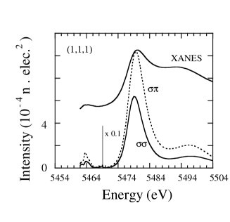
FIG. 6.: Intensity of the $(1,1,1)_{\sigma\sigma}$ (full line) and $(1,1,1)_{\sigma\pi}$ (dotted line) reflections at the vanadium K edge calculated with the orbital ordering of Eq. (35). The Bragg peaks have the same energy scale as the XANES spectra (full line). The big structure at the 4p edge is not present in the experiment. The calculation is performed with a 3 Å cluster radius.

Our results for the $(1,1,1)_{m}$ reflection are shown in Fig. 6. As in the experiment,[16] a structure is obtained at the 3d-energy level. Yet, a much bigger signal is present at the 4p edge where the experimental intensity shows no features. Such a disagreement is the proof that the OO cannot be responsible of the signal: The time-reversal breaking OO makes the $(111)_{m}$ reflection allowed not only at the 3d-energy level, but also at the 4p-energies. Note that this result remains valid for any time-reversal breaking OO, not only the one proposed in Eq. (35), as should have been qualitatively expected. Indeed, it has already been shown[10, 40] that the 3d-4p hybridization, even if small, must give a contribution to the dipolar K edge signal. In fact, previous numerical simulations in another compound, LaMnO₃, have shown that the effect of a symmetry-breaking OO of 3d orbitals produces a signal also at the 4p-energy levels. In this latter case the contribution coming from the Jahn-Teller distortion overwhelms the OO signal. However in the present case, since V₁ and V${}_{1^{\prime}}$ have the same local distortion, such a signal should have been detected, as clear from our numerical simulation shown in Fig. 6. Thus, the experimental evidence of absence of any signal at the 4p energies proves two facts: first, there is no time-reversal breaking OO; second, the (111)_m cannot be due to OO. A direct consequence of the previous analysis is that no magnetoelectric s ubgroups are compatible with the (111)_m energy scan, as they all break the time-reversal symmetry, in keeping with the negative experimental evidence for magnetoelectricity in V₂O₃.[41] This strongly supports the results of Ref. [[21]].

Notice that a previous study[42] on the same reflection in V₂O₃ ended up with the conclusion that the OO was responsible of the signal. Unfortunately that calculation was performed only around the 3d-energy range, where the agreement in the azimuthal scan was quite good and the big feature at the 4p energies was not detected. The lesson to be drawn from this fact is that the azimuthal scan around the diffraction vector is not always a fundamental feature in determining the origin of the reflection. In fact, it usually reflects more the geometry than the electronic properties of the material. This is a rather general comment, not limited to V₂O₃: when there are only one or two ab initio independent factors (the tensor components), the angular properties are much more determined by the geometry (ie, the symmetries) than by the dynamics (ie, the relative weight of the radial matrix elements). In this situation only the combined analysis of both energy and azimuthal scans is a reliable tool to investigate the electronic origin of RXS phenomena.

IV Conclusion

The main results of the present paper can be inferred from the conclusions of the last two subsections discussing the results appeared in the literature. In fact, up to now, it was possible to classify the interpretations of the forbidden Bragg reflections with $h+k+l=$odd and $h=$odd along two main lines of thought: those who explained such reflections in terms of orbital ordering, both associated[18] or not[9] with a reduction of the magnetic symmetry, and those who were inclined to a magnetic origin.[19, 20] A third explanation, that of the antiferroquadrupolar ordering proposed in Ref. [[8]] had already been ruled out in Ref. [[18]]. Whether the former or the latter interpretations were correct, was not simple to decide on the basis of the azimuthal scans, only. In fact, such scans, for a given multipolar channel, measure the crystal symmetry, rather than the electronic origin of the reflections. The proof of such a statement is that three different mechanisms (magnetic in the qq channel[19], magnetic in the dq channel[20] and non-magnetic, via orbital ordering[42]) gave all a rather good agreement in the azimuthal scan at the pre-K edge. What definitively rules out the OO origin of such reflections is the energy scan shown in Fig. 6. As noted previously, a direct consequence of this result is that no reduction of the magnetic space group $P2/a+{\hat{T}}\{{\hat{E}}|t_{0}\}P2/a$ is present. [21, 41]

The second important result of the present paper lies in the fact that we were able to make a complete ab-initio analysis of all $h+k+l=$odd reflections, starting from the crystal and magnetic structure, only. We showed that their origin (whether dd, dq or qq) strongly depends on the kind of reflection (ie, $h=$even or $h=$odd), photon energy and azimuthal angle. For $h=$odd, the dq channel is predominant, in keeping with the cluster calculations of Tanaka.[20] In spite of this particular agreement, we believe that it is important to stress that our approach goes beyond the cluster calculations performed in Ref. [[20]] as well as the simple fitting procedure of Ref. [[19]]. In fact only by means of an ab-initio procedure it is possible to cover all the main experimental evidence, ie, the azimuthal behaviour, the energy profiles, and the order of magnitude of the intensity, that is well in keeping with the rough estimate given in Ref. [[16]].

We would like to acknowledge L. Paolasini for several useful discussions.

REFERENCES

- [1] M. Imada, A. Fujimori, and Y. Tokura, Rev. Mod. Phys. 70, 1039 (1998)
- [2] D. Gibbs, D. R. Harshman, E. D. Isaacs, D. B. Mc Whan, D. Mills and C. Vettier, Phys. Rev. Lett. 61, 1241 (1988).
- [3] J. P. Hannon, G. T. Trammell, M. Blume and D. Gibbs, Phys. Rev. Lett. 61, 1245 (1988).
- [4] Y. Murakami, H. Kawada, H. Kawata, M. Tanaka, T. Arima, Y. Moritomo and Y. Tokura, Phys. Rev. Lett. 80, 1932 (1998); Y. Murakami, J. P. Hill, D. Gibbs, M. Blume, I. Koyama, M. Tanaka, H. Kawata, T. Arima, Y. Tokura, K. Hirota and Y. Endoh, Phys. Rev. Lett. 81, 582 (1998).
- [5] K. Hirota, N. Oumi, T. Matsurama, H. Nakao, Y. Wakabayashi, Y. Murakami and Y. Endoh, Phys. Rev. Lett. 84, 2706 (2000).
- [6] R. Caciuffo, L. Paolasini, A. Sollier, P. Ghigna, E. Pavarini, J. van der Brink, M. Altarelli, Phys. Rev. B 65, 174425 (2002)
- [7] S. Ishihara, and S. Maekawa, Phys. Rev. B 62, 5690 (2000); Rep. Prog. Phys. 65, 561 (2002)
- [8] S.Y. Ezhov, V.I. Anisimov, D.I. Khomskii, and G.A. Sawatzky, Phys. Rev. Lett. 83 4136 (1999)
- [9] F. Mila, R. Shiina, F.-C. Zhang, A. Joshi, M. Ma, V. Anisimov and T. M. Rice, Phys. Rev. Lett. 85, 1714 (2000).
- [10] M. Benfatto, Y. Joly and C. R. Natoli, Phys. Rev. Lett. 83, 636 (1999).
- [11] M. Takahashi, M. Usuda and J. Igarashi, Phys. Rev. B 67, 064425 (2003).
- [12] J.H. Wood and A.M. Boring, Phys. Rev. B 18, 2701 (1978).
- [13] Y. Joly, Phys. Rev. B 63, 125120 (2001).
- [14] The program can be freely downloaded at the web address http:/www-cristallo.grenoble.cnrs.fr/simulation.
- [15] M. Fabrizio, M. Altarelli and M. Benfatto, Phys. Rev. Lett. 80, 3400 (1988);
- [16] L. Paolasini, C. Vettier, F. de Bergevin, F. Yakhou, D. Mannix, A. Stunault, W. Neubeck, M. Altarelli, M. Fabrizio, P. A. Metcalf and J. M. Honig, Phys. Rev. Lett. 82, 4719 (1999).
- [17] L. Paolasini, S. Di Matteo, C. Vettier, F. de Bergevin, A. Sollier, W. Neubeck, F. Yakhou, P. A. Metcalf and J. M. Honig, J. Electron Spectrosc. Relat. Phenom. 120/1-3, 1 (2001).
- [18] S. Di Matteo, N. B. Perkins and C. R. Natoli, Phys. Rev. B 65, 54413 (2002).
- [19] S.W. Lovesey, K.S. Knight, and D.S. Sivia, Phys. Rev. B 65, 224402 (2002)
- [20] A. Tanaka, J. Phys. Soc. Jpn 71, 1091 (2002)
- [21] S. Di Matteo, Y. Joly, C.R. Natoli, Phys. Rev. B 67, 195103 (2003)
- [22] D. B. Mc Whan, T. M. Rice and J. P. Remeika, Phys. Rev. Lett. 23, 1384 (1969); D. B. Mc Whan and J. P. Remeika, Phys. Rev. B 2, 3734 (1970); A. Jayaraman, D. B. Mc Whan, J. P. Remeika and P. D. Dernier, ibid. 2, 3751 (1970).
- [23] C. Castellani, C.R. Natoli and J. Ranninger, Phys. Rev. B 18, 4945 (1978); ibid. 18, 4967 (1978); ibid. 18, 5001 (1978).
- [24] J.-H. Park, L.H. Tjeng, A. Tanaka, J.W. Allen, C.T. Chen, P. Metcalf, J.M. Honig, F.M.F. de Groot, and G.A. Sawatzky, Phys. REv. B 61, 11506 (2000)
- [25] The magnetic dipole term can be safely neglected in the x-ray range
- [26] M. Blume, in Resonant Anomalous X-ray scattering, edited by G. Materlik, J. Sparks and K. Fisher (Elsevier, Amsterdam, 1994), p. 495.
- [27] J. Garcia, G. Subias, M.G. Proietti, J. Blasco, H. Renevier, J.L. Hodeau, and Y. Joly, Phys. Rev. B 63, 054110 (2001)
- [28] S. Di Matteo, T. Chatterjee, Y. Joly, A. Stunault, J.A. Paixao, R. Suryanaryanan, G. Dhalenne, and A. Revcolevschi, Phys. Rev. B 68, 024414 (2003)
- [29] D.H. Templeton and L.K. Templeton, Acta Crystallogr. A 36, 237 (1980); V.E. Dmitrienko, Acta Crystallogr. A 39, 29 (1983)
- [30] Y. Joly, D. Cabaret, H. Renevier, C. R. Natoli, Phys. Rev. Lett. 82, 2398 (1999).
- [31] J. G. Garcia, G. Subias, M. G. Proietti, H. Renevier, J. L. Hodeau, Y. Joly, J. Blasco, M. C. Sanchez and J. F. Bérar, Phys. Rev. Lett. 85, 578 (2000).
- [32] C. R. Natoli, M. Benfatto and S. Doniach,. Phys. Rev. A 34, 4682 (1986).
- [33] S. Di Matteo, C.R. Natoli, J. Synchr. Rad. 9 9 (2002)
- [34] T. A. Tyson, K. O. Hodgson, C. R. Natoli and M. Benfatto, Phys. Rev. B 46, 5997 (1992).
- [35] U von Barth and L. Hedin, J. Phys. C: Solid State Phys. 5, 1629 (1972)
- [36] P. D. Dernier and M. Marezio, Phys. Rev. B 2, 3771 (1970).
-
[37]
The fact that is
proportional to the angular orbital moment can be shown as follows.
Using the identity:
the right hand side is the usual expression for magnetic circular dichroism in the dipole channel, which can be shown [33] to be proportional to at the K-edge. - [38] R. M. Moon, Phys. Rev. Lett. 25, 527 (1970).
- [39] Wei Bao, C. Broholm, G. Aeppli, S. A. Carter, P. Dai, T.F. Rosenbaum, J.M. Honig, P. Metcalf, S.F. Trevino, Phys. Rev. B 58, 12727 (1998).
- [40] I.S. Elfimov, V.I. Anisimov and G.A. Sawatzky, Phys. Rev. Lett. 82, 4264 (1999).
- [41] S. Di Matteo, A.G.M. Jansen, Phys. Rev. B 66, R100402 (2002)
- [42] M. Cuozzo, Y. Joly, E. K. Hlil and C. R. Natoli, in Theory of Computation for Synchrotron radiation Spectroscopy, edited by M. Benfatto, C. R. Natoli and E. Pace, Proc. A.I.P., 514, 45 (Frascati, Italy, Sept. 1999).