Applications of adiabatic passage
in solid-state devices

Abstract

Coherent population transfer by adiabatic passage is a well-known method in quantum optics. This remarkable technique which is based on simple ideas has remained largely unknown to solid-state physicists. Here we provide an introduction to the basic principles of this method and discuss also some applications in solid-state systems.
PACS number(s): 32.80.Qk, 73.23.-b, 73.40.Gk

1 Introduction

Traditionally solid-state physics is focused on systems with quasi-continuous energy spectra for the various elementary excitations present in macroscopic solids. During the past decade, however, the successful development of nanotechnology has made it possible to study devices below the micrometer scale, to manipulate single charges and fluxes, or to build small electrical and mechanical resonators. The typical energy scales for such devices are, say, on the order of 0.1 …1 Kelvin and therefore much larger than the smallest temperatures that can be reached in an experiment. Consequently, the discrete nature of the energy spectrum needs to be taken into account in order to understand the behavior of these devices.

Another interesting aspect of solid-state systems at the nanoscale is that they may exhibit quantum coherence phenomena. These new effects have attracted significant attention in the recent past. Controlling quantum coherence in solid-state nanodevices is one of the major objectives in present-day research. Achievement of this goal would make it possible to study quantum dynamics on a macroscopic scale, to provide better insight into the mechanisms of decoherence, and possibly to realize quantum information processing in practice.

A consequence of this evolution is that methods used, e.g., in quantum optics become directly relevant also in solid-state physics. A particularly interesting technique is the so-called stimulated Raman adiabatic passage (STIRAP) that has been developed by Bergmann and co-workers BergBuch ; BergRMP . This method can be used to change the quantum state of a system by controlling certain coupling parameters. The mathematics underlying this technique is rather simple and general such that it may apply to physically completely different situations.

Until now, adiabatic passage has had only very few applications in solid-state devices, e.g., Tobias1 ; Tobias2 ; NonAbel ; Alec . However, one may hope that this method, due to its elegance and simplicity, will attract more interest and find new applications to solid-state systems in the near future. In this contribution we provide a brief introduction to the basic principles of adiabatic passage. In Section 2 we will explain population transfer in three-level atoms, as it is known from quantum optics. In Section 3, the method is ‘translated’ to a simple solid-state device, a superconducting Cooper-pair box with three islands. We will show that adiabatic charge transfer between the islands is possible in close analogy to the three-level atom. Finally, in Section 4 we will briefly discuss two advanced applications that are based on the technique of adiabatic passage. In our opinion, these applications may serve to illustrate the enormous potential of the method in the field of condensed-matter physics.

2 Adiabatic Passage in Three-Level Atoms

In this section, we briefly discuss the basics of adiabatic passage. A more complete discussion of the underlying physics can be found, e.g., in the review articles Refs. BergBuch ; BergRMP and in the textbook Ref. Scully .

Consider an atom with a $\Lambda$-type three-level configuration as shown in Fig. 1. The long-lived ground states $|0\rangle$ and $|1\rangle$ (energies $\omega_{0}$, $\omega_{1}$) are coupled to an excited state $|e\rangle$ (energy $\omega_{e}$) via (classical) laser fields with Rabi frequencies $\Omega_{0}$, $\Omega_{1}$. The laser frequencies are assumed to have the same detuning $\Delta$ with respect to the atomic transitions

$$\Delta=(\omega_{e}-\omega_{0})-\nu_{0}=(\omega_{e}-\omega_{1})-\nu_{1}\ \ .$$

Figure 1: Three-level atom with two ground states $|0\rangle$, $|1\rangle$ coupled to an excited state $|e\rangle$ via laser fields $(1/2)\Omega_{0}\exp{(-i\nu_{0}t)}$, $(1/2)\Omega_{1}\exp{(-i\nu_{1}t)}$. Note that there is no direct coupling between the states $|0\rangle$ and $|1\rangle$.

If the state $|\psi(t)\rangle$ of the atom is written in the form

$$|\psi(t)\rangle\ =\ c_{e}(t)e^{-i(\omega_{e}-\Delta)t}|e\rangle\ +\ c_{0}(t)e^{-i\omega_{0}t}|0\rangle\ +\ c_{1}(t)e^{-i\omega_{1}t}|1\rangle\ \ ,$$ (1)

the equation of motion for the system (atom $+$ laser fields) in the rotating frame reads

$$i\dot{c_{e}}\ = \ (1/2)(2\Delta\ c_{e}\ +\ \Omega_{0}\ c_{0}\ +\Omega_{1}\ c_{1})$$ (2)

$$i\dot{c_{0}}\ = \ (1/2)\ \Omega_{0}\ c_{e}$$ (3)

$$i\dot{c_{1}}\ = \ (1/2)\ \Omega_{1}\ c_{e}$$ (4)

where we have neglected finite lifetimes of the atomic levels. The corresponding Hamiltonian written in the basis $\{|e\rangle,|0\rangle,|1\rangle\}$ is

$$H\ =\ \frac{1}{2}\left[\begin{array}[]{ccc}2\Delta&\Omega_{0}&\Omega_{1}\\ \Omega_{0}&0&0\\ \Omega_{1}&0&0\end{array}\right]\ \ .$$ (5)

The eigenenergies of this Hamiltonian are easily found to be

$$E^{0}=0\ \ \ \ \mathrm{and}\ \ \ E^{\pm}=\frac{1}{2}\left(\Delta\pm\sqrt{\Delta^{2}+\Omega_{0}^{2}+\Omega_{1}^{2}}\right)\ \ .$$ (6)

Note that one of the two zero diagonal elements of the Hamiltonian (5) survives independently of the couplings $\Omega_{j}$ and the offset $\Delta$. The corresponding eigenstate (which is not the ground state) reads

$$|\phi^{0}\rangle\ =\ \frac{1}{\sqrt{\Omega_{0}^{2}+\Omega_{1}^{2}}}\ (\ \Omega_{1}\ |0\rangle\ -\ \Omega_{0}\ |1\rangle\ )\ \ .$$ (7)

The remarkable property of this state is that it does not contain an admixture of the basis vector $|e\rangle$. Therefore it cannot decay by spontaneous emission from $|e\rangle$ and is usually called a ‘dark state’. The direction of $|\phi^{0}\rangle$ in the subspace $\{|0\rangle,|1\rangle\}$ is given by the (possibly complex) coupling parameters $\Omega_{j}$.

Now consider the case of weakly time-dependent coupling parameters. If the inverse characteristic scale of this time dependence is smaller than the level spacing $\Omega_{\mathrm{eff}}$ of the Hamiltonian (5)

$$\left|\frac{\dot{\Omega_{j}}}{\Omega_{j}}\right|\ll\Omega_{\mathrm{eff}}\sim|\Omega_{j}|$$ (8)

the adiabatic theorem guarantees that a given state follows the time evolution of the coupling coefficients. Consequently, the dark state can be rotated in the subspace $\{|0\rangle,|1\rangle\}$ by slowly changing the values of the couplings. Again, this is remarkable as the quantum state can be controlled by varying classical system parameters.

Population transfer from the state $|0\rangle$ to the state $|1\rangle$ can be achieved by applying the so-called counterintuitive scheme. The system is prepared in the state $|0\rangle$ at vanishing couplings. Switching on the laser 1 to a finite $\Omega_{1}$ does not affect the state of the system. Now, also the laser 0 is slowly switched on (finite $\Omega_{0}$) while $\Omega_{1}$ is turned off. As can be immediately read off Eq. (7) the dark state $|\phi^{0}\rangle$ starts to rotate towards the state $|1\rangle$. At the end of the switching procedure we have $\Omega_{1}=0$, finite $\Omega_{0}$, and the final state equals $|1\rangle$.

3 Analogy for a Cooper-pair box with three islands

Our aim is to show that Hamiltonians similar to Eq. (5) can be ‘tailored’ in solid-state devices. As an example we consider a superconducting Cooper-pair box with three islands. The (single-island) Cooper-pair box is a well-known system as it is a promising candidate for the practical realization of a solid-state qubit (see, e.g., YuriRMP and references therein).

The circuit of a three-island Cooper-pair box is shown in Fig. 2. The superconducting islands (1) and (2) are coupled via tunable Josephson junctions to the third island (e). Moreover, there is a capacitive coupling $C_{K}$ between the islands (1) and (2) which is required to generate an appropriate energy level structure of the device. The junction between island (e) and superconducting lead serves only to change the total charge on the three-island setup. The SQUID-loop layout of the junctions (1) and (2) makes it possible to control the coupling energies $E_{J1}$, $E_{J2}$ by means of the external fluxes $\Phi_{1}$, $\Phi_{2}$. The electrostatic potentials of the islands can be changed through the gate voltage sources $V_{gj}$ ($j=1,2,e$) which induce offset charges $n_{xj}=C_{gj}V_{gj}/2e$, $n_{xe}=CV_{e}/2e$ on the islands (in units of Cooper-pair charges).

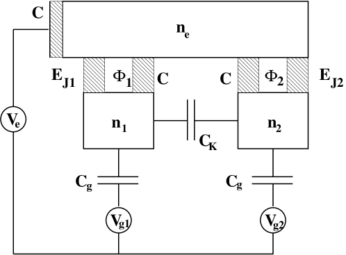
Figure 2: Circuit for a Cooper-pair box with three islands. For simplicity we choose equal gate capacitances $C_{g}$ and also equal junction capacitances $C\gg C_{g}$. The system is operated in the charge regime $E_{C}\gg E_{Jj}$. The $\Lambda$ scheme can be recognized by looking at the position of the excess Cooper pair (for a detailed explanation, see text): $|0\rangle=$ pair in island (1), $|1\rangle=$ pair in island (2), $|e\rangle=$ pair in island (e).

Let us calculate the energy of the circuit in Fig. 2 according to classical electrostatics. We assume $C_{g1}=C_{g2}=C_{g}\ll C_{1}=C_{2}=C$ and $C_{g}\ll C_{K}$. Then the electrostatic energy can be written in terms of the number of island charges $n_{j}$ (more precisely: excess charges) as

$${\cal E}(N,n_{1},n_{2}) \simeq E_{C}\left\{(N-N_{x})^{2}+\frac{C+C_{K}}{C+2C_{K}}\left[(n_{1}-n_{x1})^{2}+(n_{2}-n_{x2})^{2}\right]\right.$$ (10)

$$\ +\ \left.\frac{2C_{K}}{C+2C_{K}}(n_{1}-n_{x1})(n_{2}-n_{x2})\ +\mathrm{const.}\right\}$$

where $E_{C}=(2e)^{2}/(2C)$ denotes the charging-energy scale and $N\equiv n_{e}+n_{1}+n_{2}$ is the total charge number on all three islands (and correspondingly $N_{x}\equiv n_{xe}+n_{x1}+n_{x2}$). Observe that the number of island charges $n_{j}$ are discrete variables.

Assume we choose $N_{x}\simeq 1$. Then, the charge states with the lowest electrostatic energy correspond to a total charge of $N=1$. If we further put $n_{x1}=n_{x2}=0.4$ the charge states with $n_{1}=1$, $n_{2}=0$ (and, correspondingly, $n_{1}=0$, $n_{2}=1$) have the same energy.

In summary, we have obtained that, given the offset charges mentioned above, the three charge charge states with the lowest electrostatic energy are $|0\rangle$ with “one charge on island 1, no charge on island 2”, $|1\rangle$ with “no charge on island 1, one charge on island 2”, and $|e\rangle$ with zero excess charge on both islands 1 and 2. All other charge states have energies that are on the order of $E_{C}$ higher. Note that ${\cal E}(1,1,1)-{\cal E}(1,1,0)>{\cal E}(1,0,0)-{\cal E}(1,1,0)$.

Now we include also Josephson tunneling in our discussion. The device is to be operated in the charge regime, that is

$$\ \ \ \ \ \ \ \ E_{Jj}\ \ll\ E_{C}\ \ .$$ (11)

If we are interested in the low-energy dynamics it is sufficient to consider only the lowest-lying charge states and the relevant Josephson couplings. This is in complete analogy with the reasoning for the one-island Cooper-pair box in Ref. YuriRMP . The resulting Hamiltonian that describes the quantum dynamics of the circuit in Fig. 2 is

$$H\ = \ {\cal E}(1,0,0)|e\rangle\langle e|+{\cal E}(1,1,0)|0\rangle\langle 0|+{\cal E}(1,0,1)|1\rangle\langle 1|-$$ (13)

$$-(E_{J1}/2)(|e\rangle\langle 0|+|0\rangle\langle e|)-(E_{J2}/2)(|e\rangle\langle 1|+|1\rangle\langle e|)\ \ ,$$

where the first line describes the charging part discussed above, and the second line is the tunneling Hamiltonian in the three-dimensional subspace. As it is possible to choose ${\cal E}(1,1,0)={\cal E}(1,0,1)$, we see that the Hamiltonian Eq. (13) has exactly the same structure as the Hamiltonian Eq. (5) of the three-level atom in the rotating frame.

From the mathematical equivalence of the Hamilton operators in Eqs. (5) and (13) we conclude that an adiabatic population transfer as described in Section 2 is possible also in the three-island Cooper-pair box. Here, switching the coupling parameters means to vary the Josephson tunnel couplings by tuning the local fluxes $\Phi_{1}$, $\Phi_{2}$. Physically, the population transfer corresponds to moving the excess Cooper pair from island 1 to island 2.

4 Solid-State Applications of Adiabatic Passage

In this section, we will illustrate further applications of adiabatic population transfer in solid-state devices. It is evident from these examples that the method provides unexpected solutions to interesting problems, therefore one might hope that it finds a wider range of condensed-matter applications in the future.

4.1 Non-Abelian Holonomies by Sequences of Adiabatic Population Transfers

It is certainly an interesting problem to demonstrate the existence of geometric phases and to measure them quantitatively Shapere . Numerous manifestations of geometric phases in physics are so-called Berry phases Berry . This phase occurs when a non-degenerate quantum state carries out a cyclic evolution due to cyclic adiabatic parameter changes of the Hamiltonian.

The generalization of the Berry phase to degenerate states is the non-Abelian holonomy WilczekZee84 . Consider a quantum system which depends on an $n$-tuple of parameters $\{\lambda_{1},\ldots,\lambda_{n}\}$ (external fields, etc.), the control manifold. Moreover, let the system have a degenerate subspace which remains degenerate for any parameter point of the control manifold (this is a rather non-trivial assumption). We prepare the system in a state that is an element of the degenerate subspace and perform a cyclic adiabatic evolution of the Hamiltonian along a closed contour in the control manifold.

While a non-degenerate state returns to the initial state (times a phase factor) at the end of the cyclic evolution (a consequence of the adiabatic theorem), a state in the degenerate subspace will, in general, experience a rotation $U$ within the degenerate subspace. This rotation is called a non-Abelian holonomy. Mathematically $U$ is given by a path-ordered integral along the contour $C$

$$U\ =\ {\cal P}\ \exp{\oint_{C}\chi\ \mathrm{d}\lambda}$$ (14)

where $\chi$ is the (matrix-valued) Wilczek-Zee connection WilczekZee84 . In general this expression is rather difficult to evaluate. Therefore, it is an interesting question whether one can find contours in the control manifold for which one can immediately see the corresponding holonomy $U$. This is of relevance also for an experimental demonstration of non-Abelian holonomies.

Adiabatic passage provides an answer to this question that has been found in the context of holonomic quantum computation Unanyan99 ; Duan01 ; NonAbel . Consider a four-level scheme with states $|e\rangle$, $|1\rangle$, $|2\rangle$, $|3\rangle$ (see Fig. 3a) where the control manifold is given by the coupling parameters $\{J_{1},J_{2},J_{3}\}$. This system can be realized, e.g., in a superconducting nanocircuit with three islands in analogy with the circuit in Fig. 2 (see also Ref. NonAbel where a similar system has been studied).

Figure 3: (a) Four-level scheme for the generation of non-Abelian holonomies. The energies of the levels (i.e., the diagonal elements of the 4$\times$4 Hamiltonian analogous to Eq. (5)) are $E_{e}=\varepsilon$ and $E_{1}=E_{2}=E_{3}=0$. (b) Contour in the control manifold described in the text. The starting point is $J_{1}=J_{3}=0$, $J_{2}$ finite.

It is easy to show that this system has a two-dimensional degenerate subspace for any parameter configuration in the control manifold. The system is prepared in the state $|1\rangle$ and $J_{1}=0$, $J_{2}=\cal J$, $J_{3}=0$. Now we perform a 3-step sequence of adiabatic passages (cf. also Fig. 3b):

• 1st step: switch off $J_{2}$ while $J_{1}$ is switched on
                                $\longrightarrow$ state of system changes $|1\rangle\rightarrow|2\rangle$

• 2nd step: switch off $J_{1}$ while $J_{3}$ is switched on
                                $\longrightarrow$ state of system does not change

• 3rd step: switch off $J_{3}$ while $J_{2}$ is switched on
                                $\longrightarrow$ state of system changes $|2\rangle\rightarrow|3\rangle$

We see that, while a closed contour is described in the control manifold, the state of the system is rotated from state $|1\rangle$ to state $|3\rangle$ (possibly times a phase factor). That is, we have found a simple non-Abelian holonomy which can be generated experimentally in a straightforward manner.

4.2 Coupled Quantum Dots

Another solid-state application is the realization of dark states and adiabatic passage in coupled quantum dots. The original proposal Tobias1 with two coupled quantum dots in the strong Coulomb blockade regime is actually quite close to three-level systems in atoms, with the additional possibility to test the effect (and its modifications) in electronic transport, cf. Fig. 4. The dark state  Eq. (7) appears in the form of a sharp anti-resonance in the stationary current through a double dot as a function of the ‘Raman detuning’, i.e. the detuning difference of the two classical laser (or microwave) fields. The half-width of the anti-resonance can then be used to extract valuable information, such as the relaxation and dephasing times of tunnel coupled dot-ground state superpositions, from transport experiments.

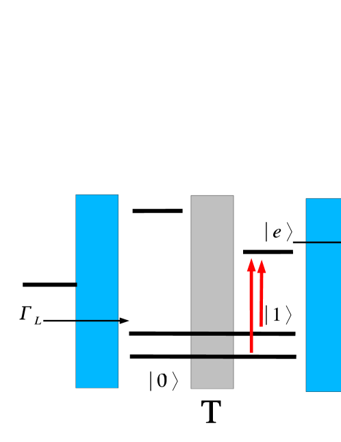
Figure 4: Dark states and STIRAP through two tunnel ($T$) coupled dots in the Coulomb blockade regime with hybridized states $|0\rangle$, $|1\rangle$. Electrons tunnel in from the left, are photo-pumped to the excited state $|e\rangle$, and tunnel out to the right.

Using two time-dependent Stokes and pump pulses, an extension of the counterintuitive STIRAP scheme has subsequently been suggested for this configuration Tobias1 , taking into account a finite decoherence rate $\gamma$ due to, e.g. electron-phonon coupling in the dots. In principle, $\gamma$ can be obtained from monitoring the time-dependent electronic current through the dots, which however is quite weak for small $\gamma$, when the dot is essentially trapped in the dark superposition of $|0\rangle$ and $|1\rangle$. An alternative way is to apply a second pair of simultaneous pulses with amplitude ratios that give either zero or full current in the coherent case $\gamma=0$. The deviation from the ‘zero/full’ current situations then gives rise for a current ‘contrast’ from which $\gamma$ can be extracted.

Another adiabatic scheme that completely avoids the use of lasers or microwaves has been introduced in quantum dots which are coupled by slowly varying static tunnel barriers. In fact, the rotating wave approximation in the original (optical) population transfer scheme leads to time-independent (or slowly parametric) Hamiltonians like  Eq. (5), where fast terms are already transformed away. This makes it obvious that one can start from time-dependent tunnel couplings right from the beginning. In the simplest realization Tobias2 , one considers three single level dots $L$, $C$, $R$ in a line, with two time-dependent couplings $T_{i}(t)$ between $C$ and $i=L,R$ which are then switched on and off with a time-delay as in the STIRAP scheme. The resulting adiabatic transfer of charge from the left to the center to the right can then essentially be understood in terms of level-crossings of the (instantaneous) three eigenvalues of the energy. If the tunnel coupling remains small but finite in the ‘off’ periods, these level crossings become anti-crossings. Already for the two-level system in a double quantum dot, one realizes that one actually has to deal with (dissipative) Landau-Zener tunneling between curves on energy surfaces in the parameter space of the problem Tobias3 . This type of ‘pumping’, which occurs in Hilbert spaces that are essentially cut down to very small dimensions due to strong correlations, is the opposite limit of the ‘usual’ adiabatic pumping in large, non-interacting mesoscopic systems Brouwer98 .

5 Conclusions

We have outlined the basic ideas of adiabatic passage and several examples of its application in solid-state devices that can be realized in superconductor as well as in semiconductor systems. The examples showed that adiabatic passage-like techniques may be used to generate simple charge transfers, to detect non-Abelian holonomies and to control charge transport properties (in particular also to design an alternative kind of charge pumps). In our opinion, it is obvious even from these simple examples that the method of adiabatic passage has significant potential for applications in solid-state physics and deserves appropriate attention also in this field.

The authors gratefully acknowledge stimulating discussions with L. Faoro, R. Fazio, A. Kuhn, F. Renzoni, and T. Vorrath.

References

- (1) K. Bergmann and B.W. Shore: Coherent population transfer. In H.L. Dai and R.W. Field (Eds.) Molecular dynamics and stimulated emission pumping, p. 315. (World Scientific, Singapore, 1995)
- (2) K. Bergmann, H. Theuer, and B.W. Shore: Coherent Population Transfer Among Quantum States of Atoms and Molecules, Rev. Mod. Phys. 70, 1003 (1998).
- (3) T. Brandes and F. Renzoni: Current switch by coherent trapping of electrons in quantum dots, Phys. Rev. Lett. 85, 4148 (2000); T. Brandes, F. Renzoni, and R. H. Blick: Adiabatic steering and determination of dephasing rates in double-dot qubits, Phys. Rev. B 64, 035319 (2001).
- (4) F. Renzoni and T. Brandes: Charge transport through quantum dots via time-varying tunnel couplings, Phys. Rev. B 64, 245301 (2001).
- (5) L. Faoro, J. Siewert, and R. Fazio: Non-Abelian Holonomies, Charge Pumping and Quantum Computation with Josephson Junctions, Phys. Rev. Lett. 90, 028301 (2003).
- (6) M.H.S. Amin, A.Yu. Smirnov, and A. Maassen v.d. Brink: Josephson-phase qubit without tunneling, Phys. Rev. B 67, 100508(R) (2003).
- (7) M.O. Scully and M.S. Zubairy: Quantum Optics (Cambridge Univ. Press, Cambridge 1997)
- (8) Yu. Makhlin, G. Schön, and A. Shnirman: Quantum-state engineering with Josephson-junction devices, Rev. Mod. Phys. 73, 357 (2001).
- (9) A. Shapere and F. Wilczek (Eds.): Geometric phases in physics, (World Scientific, Singapore, 1989).
- (10) M.V. Berry, Quantum Phase Factors Accompanying Adiabatic Changes, Proc. Roy. Soc. A 392, 45 (1984).
- (11) F. Wilczek and A. Zee, Appearance of Gauge Structure in Simple Dynamical Systems, Phys. Rev. Lett. 52, 2111 (1984).
- (12) R.G. Unanyan, B.W. Shore, and K. Bergmann, Laser-driven population transfer in four-level atoms: Consequences of non-Abelian geometrical adiabatic phase factors, Phys. Rev. A 59, 2910 (1999).
- (13) L.-M. Duan, J.I. Cirac, and P. Zoller, Geometric Manipulation of Trapped Ions for Quantum Computation, Science 292, 1695 (2001).
- (14) T. Brandes and T. Vorrath, Adiabatic transfer of electrons in coupled quantum dots, Phys. Rev. B 66, 075341 (2002).
- (15) P.W. Brouwer: Scattering approach to parametric pumping, Phys. Rev. B 58, 10135 (1998).