Optical absorption in quantum dots:
Coupling to longitudinal optical phonons treated exactly

Abstract

Optical transitions in a semiconductor quantum dot are theoretically investigated, with emphasis on the coupling to longitudinal optical phonons, and including excitonic effects. When limiting to a finite number of $m$ electron and $n$ hole levels in the dot, the model can be solved exactly within numerical accuracy. Crucial for this to work is the absence of dispersion of the phonons. A suitable orthogonalization procedure leaves only $m(m+1)/2+n(n+1)/2-2$ phonon modes to be coupled to the electronic system. We calculate the linear optical polarization following a delta pulse excitation, and by a subsequent Fourier transformation the resulting optical absorption. This strict result is compared with a frequently used approximation modeling the absorption as a convolution between spectral functions of electron and hole, which tends to overestimate the effect of the phonon coupling. Numerical results are given for two electron and three hole states in a quantum dot made from the polar material CdSe. Parameter values are chosen such that a quantum dot with a resonant sublevel distance can be compared with a nonresonant one.

I Introduction

Quantum dots (QDs) based on semiconductor structures have received great attention for almost two decades now Koch93 . Whereas early experiments were only able to measure ensemble averages over many quantum dots, it is nowadays possible to address single quantum dots individually BCWB92 . Photoluminescence and more recently absorption Guest has been measured with high spatial resolution, showing distinct lines related to individual dots (due to well width fluctuations in a quantum well). Using magneto-photoluminescence, detailed information on energy levels and phonon coupling could be extracted for single QDs made from II-VI semiconductor material FlissHen01 . This and related experimental work has enormously stimulated investigations on the interaction between the carriers on confinement levels and the surrounding polarizable medium on a microscopic level. A proper understanding of the related dephasing mechanisms might become important in view of future quantum computation applications based on semiconductor quantum dots Jacak05 .

Carrier relaxation and dephasing in quantum dots crucially depends on the interaction with lattice vibrations (phonons). At first sight, scattering with longitudinal-optical (LO) phonons seems to be possible only if a sublevel spacing matches the LO phonon energy $\hbar\omega_{0}$. In other (non-resonant) cases, scattering is expected to be impossible (or at least strongly reduced). This is the so-called phonon-bottleneck problem which has been discussed intensively in the literature BB90 . The argument relies on the application of Fermi’s golden rule which demands energy conservation in each individual process. However, electron-phonon interaction in quantum confined systems SMC87 ; VFB02 gives rise to a far more complicated picture including: Non-Markovian scattering, formation of electron-phonon bound states with level repulsion, and phonon satellites spaced at multiples of $\hbar\omega_{0}$.

The coupling of quantum dot levels to acoustic phonons is responsible for another set of features. Due to their dispersion, the possible energy transfer covers a range from zero to a maximum value (typically, a few meV) which is related to the dot size. Consequently, phonon satellites appear here as broad bands surrounding the zero-phonon line Besombes ; Axt . The broadening of this line itself is a subject of intense research. Similar to the phonon bottleneck problem mentioned above, an advanced theory MZ04 predicts a finite broadening even in cases where the next confined level is far away in energy compared to the maximal possible energy transfer.

In the present work, we want to focus on the interaction with LO phonons. This is relevant for quantum dots made from polar material like CdSe, where the Fröhlich interaction with LO phonons is much stronger than the coupling to acoustic phonons. Král et al. KK98 have dealt with the LO phonon bottleneck problem and found within a standard self energy approach (second order in the interaction) an appreciable broadening of the levels which persists even outside the exact resonance. It has further been argued that relaxation properties can be obtained from a convolution of the spectral functions of the discrete energy levels.

Aiming at a non-perturbative treatment, a big advantage is the dispersionless nature of the LO phonons which allows a numerically exact treatment. We have derived in our previous paper Ref. SZC00, an efficient scheme to calculate eigenenergies and eigenvectors, which rests upon a unitary transformation of the phonons into a new set where only a few modes are coupled to the electronic degrees of freedom. We have calculated the electron spectral function and shown that it consists of a series of discrete delta functions. They are distributed around the bare level energies and at multiples of the LO energy (phonon satellites). Under resonance conditions, the eigenenergies are still split in form of avoided level crossing. This is reminiscent to the Rabi splitting in a two-level system coupled to monochromatic photons (which formally replace the phonons). The self consistent second Born approximation for the self energy gives some gross features of the spectrum but has broadened levels instead of the closely spaced discrete lines in the exact calculation. Thus, we had concluded that this approximation fails if phonons are coupled to discrete electronic levels. Recently, our numerically exact treatment was used to assess results obtained via the Davydov’s canonical transformation Jacak03 .

Looking at the influence of phonon interaction on the interband transitions, one has to refer to a seminal paper by Schmitt-Rink and coworkers SMC87 . They have shown that the phonon interaction in general will increase with confinement (i.e. with reducing the dot size). For the Fröhlich coupling to LO phonons, however, things are more subtle since here the difference in charge distribution between initial (valence band sublevel) and final state (conduction band sublevel) enters. Now, under strong confinement, the sublevel wave functions are getting more similar. Therefore, the optical transition is accompanied with practical no change in local charge distribution, and the net LO phonon coupling is drastically reduced.

In Ref. KK98 , it has been claimed that the interband absorption spectrum can be taken as a convolution of the one-particle spectral functions for the electron and the hole. In the present work which extends Ref. SZC00 to a two-band many-level situation, and allows to calculate the linear optical response exactly, we will demonstrate the failure of this convolution approach. Indeed, it is missing the correct charge redistribution.

Absorption in QDs was first discussed in Ref. Fom98 with emphasis on the non-adiabatic electron-phonon coupling, labeled as phonon-assisted transitions in Ref. SZC00 . In Ref. Jac03 , a detailed comparison between features in QDs and phenomena from quantum optics was presented, again focusing on the electron-phonon interaction. Recently, the absorption spectrum of individual QDs has been discussed for intra-band LOH05 as well as for inter-band transitions VAM04 . In the latter work, the valence band levels were treated without phonon interaction - which leads to an even simplified form of the convolution approach. However, the resonance condition (matching a sublevel distance by $\hbar\omega_{0}$) can be much easier obtained in the valence band since the sublevel spacing is here smaller than in the conduction band.

The paper is organized as follows. In section II, the model and the Hamiltonian are presented, which includes both carrier-phonon and carrier-carrier (Coulomb) interaction. In section III, we define and perform the unitary transformation which reduces the number of Bosonic modes coupled to the Fermionic states. This works if the phonons have no dispersion, and makes a numerical diagonalization of the Hamiltonian feasible. Equations for the linear polarization in terms of exact eigenstates are derived in section IV, and the approximate convolution of electron and hole spectral function is given as well. In section V, numerical results for two prototype quantum dots made from the polar material CdSe are presented and discussed. Several details on the transformations and a list of material parameters are given in the Appendix.

II The model

We start with the standard Hamiltonian which couples the band states in a semiconductor to the lattice displacement. For the quantum dot, the confined electronic states in the conduction (valence) band are given by Fermionic creation operators $c^{\dagger}_{j}\,(v^{\dagger}_{j})$. The lattice vibrations are taken as longitudinal optical phonons without dispersion, $\hbar\omega_{0}$, and represented by Bosonic operators $b_{\mathbf{q}}^{\dagger}$:

$$H = \sum_{\mathbf{q}}\hbar\omega_{0}b^{\dagger}_{\mathbf{q}}b_{\mathbf{q}}+\sum_{j}\left(\epsilon_{j}^{c}c_{j}^{\dagger}c_{j}\,+\,\epsilon_{j}^{v}v_{j}^{\dagger}v_{j}\right)$$

$$+ \sum_{\mathbf{q}jl}\left(b_{\mathbf{q}}+b_{-\mathbf{q}}^{\dagger}\right)\left(M_{\mathbf{q}jl}^{c}c_{j}^{\dagger}c_{l}+M_{\mathbf{q}jl}^{v}v_{j}^{\dagger}v_{l}\right)\,.$$

The coupling matrix elements $M_{\mathbf{q}jl}^{a}\,(a=c,v)$ stem from the Fröhlich interaction applied to the confinement wave functions (see Appendix C for details). Note that there is no phonon coupling between valence and conduction band states since the energy gap is far greater than the LO phonon energy, while the distance between confined levels in one band $\epsilon_{j}^{a}-\epsilon_{l}^{a}\,(a=c,v)$ may be well in the range of the phonon energy. Electron spin is not included here since spin relaxation is a slow process compared to the spin-conserving electron-phonon interaction. Similarly, phonon-assisted transitions into the continuum of wetting layer states are not considered. For simplicity, we restrict ourselves to the interaction with bulk phonon modes, leaving the more precise picture of confined and interface modes for future investigations GKFNZGT04 .

For treating optical transitions between the filled valence band and the empty conduction band, it is convenient to switch from the conduction-valence-band description used in Eq. (II) to the electron-hole picture. This is accomplished by the replacement

$$c_{j}\rightarrow e_{j},\quad v_{j}\rightarrow h_{j}^{\dagger}\,.$$ (2)

Using $v_{j}^{\dagger}v_{l}=\delta_{j,l}-h_{l}^{\dagger}h_{j}$ the Hamiltonian is rewritten as

$$H = \sum_{\mathbf{q}}\hbar\omega_{0}b^{\dagger}_{\mathbf{q}}b_{\mathbf{q}}\,+\,\sum_{j}\left(\epsilon_{j}^{c}e_{j}^{\dagger}e_{j}-\epsilon_{j}^{v}h_{j}^{\dagger}h_{j}\right)$$ (3)

$$+ \sum_{\mathbf{q}jl}\left(b_{\mathbf{q}}+b_{-\mathbf{q}}^{\dagger}\right)\left(M_{\mathbf{q}jl}^{c}e_{j}^{\dagger}e_{l}-M_{\mathbf{q}lj}^{v}h_{j}^{\dagger}h_{l}\right)$$

$$+ \sum_{j}\epsilon_{j}^{v}\,+\,\sum_{\mathbf{q}j}\left(b_{\mathbf{q}}+b_{-\mathbf{q}}^{\dagger}\right)M_{\mathbf{q}jj}^{v}\,.$$

Note that the phonon interaction now carries a negative sign for the hole states compared to the electron states, which can be traced back to the different charge sign of the excitations. In Appendix A we show that the last line can be dropped by renormalizing the ground state energy.

As we are focusing on the linear response, the Coulomb interaction leads to the formation of a single exciton only. The relevant interaction term is

$$H^{C}=-\sum_{klij}v_{klij}e_{k}^{\dagger}h_{l}^{\dagger}h_{j}e_{i}\,,$$ (5)

and has to be added to Eq. (3). $v_{klij}$ denotes the Coulomb matrix element between sublevel states (for details, see appendix C). Under strong confinement conditions considered here, the confinement states are only reshaped marginally ZimEdinb , and the Coulomb interaction leads to almost rigid shifts of the transition energies (exciton binding energies). However, non-diagonal Coulomb couplings have to be included since they can be of similar order as the phonon couplings, and modify the oscillator strengths as well.

III Reducing the phonon subspace

The phonon coupling in Eq. (3) involves only certain combinations of phonon operators, e.g. $\sum_{\mathbf{q}}M_{\mathbf{q}jl}^{c}\,b_{\mathbf{q}}$. If we consider a finite number (say $m$) of electron sublevels in the dot, and $n$ hole sublevels, there are $m^{2}+n^{2}$ such combinations (as argued above, phonon-assisted transitions between conduction and valence bands are absent). Since we are dealing exclusively with confined states, the confinement wave functions can be chosen to be real, and the symmetry $M_{\mathbf{q}lj}^{a}=M_{\mathbf{q}jl}^{a}$ holds. This reduces the linear independent combinations to $m(m+1)/2+n(n+1)/2$.

A further reduction can be achieved since in the present Hamiltonian Eq. (3), the number of electrons ($N_{e}$) and of holes ($N_{h}$) are conserved quantities. Therefore, two (diagonal) Fermion pairs in the interaction can be expressed by the remaining ones. We choose

$$e^{\dagger}_{m}\,e_{m}=N_{e}-\sum_{j=1}^{m-1}e^{\dagger}_{j}\,e_{j}\,,\quad h^{\dagger}_{n}\,h_{n}=N_{h}-\sum_{j=1}^{n-1}h^{\dagger}_{j}\,h_{j}\,,$$ (6)

which gives additions to all the other diagonal coupling terms, and a $c$ number remainder. In order to shorten the subsequent writing, we introduce pair indices $\lambda=1,\dots,(N-2)$ which combine either two electron sublevels (e:$jl$) or two hole sublevels (h:$jl$), with $j\leq l$. Caring for the different signs in the interaction of Eq. (3), we define in the conduction band

$$M_{\mathbf{q}\lambda}=M^{c}_{\mathbf{q}\,jl}-\delta_{jl}M^{c}_{\mathbf{q}\,mm}\,,$$ (7)

and in the valence band

$$M_{\mathbf{q}\lambda}=-M^{v}_{\mathbf{q}\,lj}+\delta_{jl}M^{v}_{\mathbf{q}\,nn}\,.$$ (8)

For treating the $c$ number part properly, we have to introduce one further index $\lambda=\kappa\equiv N-1$, with the matrix element

$$M_{\mathbf{q}\,\kappa}=N_{e}M_{\mathbf{q}\,mm}^{c}\,-\,N_{h}M_{\mathbf{q}\,nn}^{v}\,.$$ (9)

Now, the interaction term of Eq. (3) reads

$$\sum_{\lambda=1}^{\kappa-1}\left(A_{\lambda}\,+\,A^{\dagger}_{\lambda}\right)\left(c^{\dagger}\,c\right)_{\lambda}\,+\,\left(A_{\kappa}\,+\,A^{\dagger}_{\kappa}\right)$$ (10)

with a shorthand writing for the Fermionic operators. Note that for the nondiagonal terms $j\neq l$, we have to set e.g.

$$(c^{\dagger}c)_{\lambda}=e^{\dagger}_{j}e_{l}+e^{\dagger}_{l}e_{j}\,.$$ (11)

The combinations of phonon operators entering Eq. (10) are

$$A_{\lambda}=\sum_{\mathbf{q}}M_{\mathbf{q}\lambda}b_{\mathbf{q}}\quad\left(\lambda=1\dots\kappa\right)\,,$$ (12)

but the $A_{\lambda}$ do not form an orthonormal set. As detailed in Appendix B, we apply the Gram-Schmidt orthonormalization scheme to generate new phonon operators $B_{\lambda}$ which are properly orthogonalized. The transformation is a linear one,

$$A_{\lambda}=\sum_{\alpha=1}^{\lambda}I_{\lambda\alpha}B_{\alpha}\,,$$ (13)

and leads to the transformed Hamiltonian

$$H = \sum_{\lambda}\hbar\omega_{0}B^{\dagger}_{\lambda}\,B_{\lambda}\,+\,\sum_{j}\left(\epsilon^{c}_{j}\,e^{\dagger}_{j}\,e_{j}\,-\,\epsilon^{v}_{j}\,h^{\dagger}_{j}\,h_{j}\right)$$

$$+ \sum_{\lambda=1}^{\kappa-1}\sum_{\alpha=1}^{\lambda}\left(I_{\lambda\alpha}B_{\alpha}\,+\,I^{*}_{\lambda\alpha}B^{\dagger}_{\alpha}\right)\left(c^{\dagger}c\right)_{\lambda}$$

$$+ \sum_{\alpha=1}^{\kappa}\left(I_{\kappa\alpha}B_{\alpha}\,+\,I^{*}_{\kappa\alpha}B^{\dagger}_{\alpha}\right)\,.$$

To arrive at the standard diagonal form of the free phonon part, it was essential that the phonons have no dispersion. Otherwise, the subset of $B_{\lambda}$ would still mix with the remaining phonon operators. These remaining degrees of freedom only contribute to the free phonon energy and are omitted from Eq. (III).

A careful inspection of Eq. (III) shows that the Bosonic operator $B_{\kappa}$ only appears as last element in the last line of Eq. (III), and in the free phonon part. It is therefore decoupled from the Hamiltonian and allows an independent solution in terms of a shifted oscillator,

$${\cal B}_{\kappa}=B_{\kappa}+I_{\kappa\kappa}/\hbar\omega_{0}\,.$$ (15)

Therefore, only

$$N=\frac{m(m+1)}{2}\,+\,\frac{n(n+1)}{2}-2$$ (16)

new modes are coupled to the Fermionic Hilbert space.

Assuming a symmetric dot shape, the confinement functions are either even or odd, and the matrix elements $M_{\mathbf{q}jl}^{a}$ have a definite parity in $\mathbf{q}$, too. Consequently, the compound matrix elements $M_{\lambda\alpha}$ defined in Eq. (46) vanish if $\lambda$ and $\alpha$ refer to different parity. Therefore, the tridiagonal matrix $K$ (and $I$ as well) has a block structure, allowing the Gram-Schmidt procedure to work in each block independently. Note that the Coulomb matrix elements have an equivalent parity, and therefore do not mix these blocks. For certain confinement potentials like the harmonic potential, the number of phonon modes can be reduced even further (see appendix C).

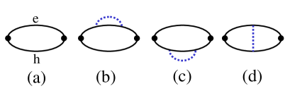
Figure 1: Diagrammatic expansion of the optical polarization up to first order in the electron-phonon interaction. Lines denote the electron (e) and hole (h) propagator, the dotted line the phonon propagator, and the large dot stands for the optical dipole matrix element. The zeroth-order diagram (a) describes interband transitions between confined states unaffected by the phonon interaction. In the convolution approach, only self-energy type diagrams (b, c) are considered, while in the full evaluation, vertex type diagrams (d) are included as well.

IV Linear optical response

In this section, we want to contrast the direct evaluation of the time-dependent linear polarization and the absorption spectrum with the so-called convolution approach: Here, only the spectral functions of the electron and hole states are calculated, and the absorption is taken as a convolution of both quantities. Before deriving the corresponding formal expressions, let us point out the main difference: For the direct evaluation, we start from the electron-hole vacuum ($N_{e}=0,N_{h}=0$) as initial state and end up in the subspace of one electron-hole pair ($N_{e}=1,\,N_{h}=1$). For the convolution approach, quite different subspaces are invoked, namely $N_{e}=0,N_{h}=0\rightarrow N_{e}=1,N_{h}=0$ for the electron spectral function, and $N_{e}=0,\,N_{h}=0\rightarrow N_{e}=0,\,N_{h}=1$ for the hole one. In diagram language, any process which has a phonon correlation between electron and hole levels is discarded in the convolution approach. In Fig. 1, we display the relevant first order diagrams. The vertex diagram Fig. 1d is the first one describing interband phonon correlations. In particular under strong confinement conditions, it compensates to a large extent the self-energy type diagrams (Fig. 1b, c). Only the latter are kept in the convolution approach and we expect much to strong phonon satellites in this approximate treatment. Formally, in the convolution approach, the matrix elements appear as $(M^{c})^{2}$ or $(M^{v})^{2}$, while the full version includes the vertex corrections containing $M_{c}M_{v}$ as well. For level-diagonal matrix elements, this combines into $(M^{c}-M^{v})^{2}$. The appearance of matrix element differences can be seen already in Eq. (3). Therefore, the near cancellation of changes in the charge distribution SMC87 can only be achieved when treating self energy and vertex diagrams on an equal footing. Note that excitonic effects are completely absent within the convolution approach.

IV.1 Direct evaluation

The coupling to the light is described within the dipole approximation for interband transitions, adding

$$E(t)\sum_{ij}(\mu_{ij}\,c_{i}^{\dagger}v_{j}\,+\,h.c.)$$ (17)

as a perturbation to the Hamiltonian. The dipole matrix elements are given by an integral over the confinement functions,

$$\mu_{ij}=\mu_{cv}\int d^{3}r\,\psi_{i}^{e}({\bf r})\,\psi_{j}^{h}({\bf r})\,,$$ (18)

having as prefactor the dipole moment between the valence and conduction band, $\mu_{cv}$.

The linear optical response follows from the polarization after a unit-area delta pulse at $t=0$ and is given as dipole-dipole-correlation function. Expressed via the electron and hole operators, we have for $t\geq 0$

$$P(t)=i\sum_{ij,kl}\mu_{kl}^{*}\,\mu_{ij}\langle h_{l}(t)\,e_{k}(t)\,e_{i}^{\dagger}(0)\,h_{j}^{\dagger}(0)\rangle$$ (19)

with the time dependence of the operators in the Heisenberg picture. The expectation value is shorthand writing for the statistical sum over initial states which contain no electron-hole pairs, and a thermal distribution of phonon mode occupations $n_{\lambda}=0,1,\dots\infty$. This is denoted by $|n_{\lambda},0\rangle$, with total energy

$$E_{0}=\hbar\omega_{0}\sum_{\lambda}n_{\lambda}\,.$$ (20)

Then, we proceed with

$$P(t)\propto i\sum_{n_{\lambda}}e^{-\beta E_{0}}\sum_{ij,kl}\mu_{kl}^{*}\mu_{ij}\langle n_{\lambda},0|h_{l}(t)e_{k}(t)|n_{\lambda},ij\rangle\,.$$ (21)

In practice, the independent summation over phonon occupations $n_{\lambda}$ can be restricted to a maximum number which depends on coupling strength and temperature, $\beta=1/k_{B}T$. For simplicity, we have omitted a prefactor which ensures the proper normalization of the statistical sum.

While the zero-pair states $|n_{\lambda},0\rangle$ diagonalize the zero-pair Hamiltonian properly, we need to look for the one-pair states from the eigenvalue problem

$$\left(H+H^{C}\right)_{1}|\phi\rangle=E_{\phi}|\phi\rangle\,.$$ (22)

Due to the reduction of the number of Bosonic modes, this can be solved numerically exact by expanding into the noninteracting one-pair basis $|n_{\lambda},ij\rangle$.

Plugging all time dependencies together, we obtain

$$P(t) = i\sum_{n_{\lambda}}e^{-\beta E_{0}}\sum_{ij,kl,\phi}\mu_{kl}\,\mu_{ij}$$

$$\times e^{i(E_{0}-E_{\phi})t/\hbar}\langle n_{\lambda},kl|\phi\rangle\langle\phi|n_{\lambda},ij\rangle\,.$$

Starting with the initial value

$$P(t=0)=i\sum_{n_{\lambda}}e^{-\beta E_{0}}\sum_{kl}|\mu_{kl}|^{2}\,,$$ (24)

the polarization evolves in time as a sum over many individual oscillations. Although each of these terms does not have a damping, in the sum a general decay can be observed (quasi-dephasing), as shown in Sec. V.

The imaginary part of the Fourier transformation of the polarization function yields the absorption spectrum,

$$\alpha(\omega) = \text{Im}\int_{-\infty}^{\infty}dt\,P(t)\,e^{i\omega t}$$

$$\propto \sum_{n_{\lambda}}e^{-\beta E_{0}}\sum_{ij,kl,\phi}\mu_{kl}^{*}\mu_{ij}$$

$$\times \langle n_{\lambda},kl|\phi\rangle\langle\phi|n_{\lambda},ij\rangle\delta(E_{\phi}-E_{0}-\hbar\omega)\,.$$ (26)

Let us point out that the exact absorption spectrum consists of delta peaks only. This was clear from the beginning since a finite perturbation cannot change the character of the spectrum of the unperturbed system. Since we started from dispersionless Bosonic modes, the discrete electronic spectrum cannot be altered by the non-zero electron-phonon interaction ReSi75 .

IV.2 Convolution approach

It has been argued in the literature KK98 , that the convolution of electron and hole spectral functions may give a reasonable approximation to the absorption spectrum,

$$\alpha^{con}(\omega)\propto\int d\omega^{\prime}\sum_{ij,kl}\mu_{kl}^{*}\,\mu_{ij}\,A_{ki}^{e}(\omega^{\prime})\,A_{lj}^{h}(\omega-\omega^{\prime})\,.$$ (27)

Indeed, avoiding the evaluation of the two-particle (i.e. dipole-dipole) correlation functions would be an important reduction of the numerical labor, since the spectral function is a genuine one-particle function. We concentrate on the electron spectral function $A_{ki}^{e}(\omega)$ which is defined by

$$A_{ki}^{e}(\omega)=\frac{1}{\pi}\,\text{Re}\int_{0}^{\infty}dt\,e^{i\omega t}\,\langle e_{k}(t)e^{\dagger}_{i}(0)\rangle\,.$$ (28)

Here, we need the exact eigenstates of the Hilbert space with $N_{e}=1,\,N_{h}=0$ which will be denoted by $H_{e}|\chi\rangle=E_{\chi}|\chi\rangle$. Similar arguments as used in deriving Eq. (IV.1) lead to

$$A_{ki}^{e}(\omega) \propto \sum_{n_{\lambda}}e^{-\beta E_{0}}$$

$$\times \sum_{\chi}\langle n_{\lambda},k|\chi\rangle\langle\chi|n_{\lambda},i\rangle\,\delta(E_{\chi}-E_{0}-\hbar\omega)\,,$$

where $|n_{\lambda},k\rangle$ is the (non-interacting) one-electron basis. Similar equations hold for the hole spectral function. Due to the assumed dot symmetry, the only off-diagonal spectral function will be the hole spectral function related to h:13.

V Numerical results

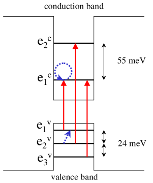
Figure 2: Schematic band diagram with sublevel spacings corresponding to the resonant quantum dot. Vertical arrows - optical transitions, dotted lines - phonon processes. For further explanation, see text.

We consider a prototype quantum dot of ellipsoidal shape with CdSe as the semiconductor material. The relevant LO phonon energy is $\hbar\omega_{0}=24\,$meV. The larger mass of the holes results in a smaller level distance in the valence band. In order to cover a comparable energy range in the conduction and the valence band, we take into account the two lowest confined states in the conduction band ($m=2$) and the three lowest confined states in the valence band ($n=3$). In accordance with Eq. (16), we then have seven new phonon modes.

According to what has been said before, there is the odd parity group ($\lambda$ = e:12, h:12, h:23) and the even parity group ($\lambda$ = e:11, h:11, h:22). The special mode $\lambda=\kappa\equiv 7$ refers to the even parity group. Consequently, $K$ and $I$ decompose into a three-dimensional block for both parity groups. Due to the harmonic potential, no extra Bosonic mode is assigned to the transition h:13 which can be expressed by other Bosonic modes (see Appendix C).

For characterizing the different dot sizes we define the first sublevel distance in each band (without phonon interaction and exciton effects) as

$$\Delta^{a}\equiv|\epsilon_{2}^{a}-\epsilon_{1}^{a}|\quad(a=c,v)\,.$$ (30)

In the sequel, we calculate the linear optical properties for two selected dot sizes: The resonant quantum dot has perfect resonance between phonon energy and sublevel distance in the valence band, $\Delta^{v}=\hbar\omega_{0}=24\,$meV, and consequently $\Delta^{c}=55\,$meV. In Fig. 2, the confinement levels for the resonant QD are shown schematically. Vertical arrows mark the nonzero optical transitions. The dotted lines denote phonon processes. In the valence band, this is resonant with the sublevel distance (real transition, driven by $M_{\mathbf{q}12}^{v}$). In the conduction band, a virtual process involving the diagonal matrix element $M_{\mathbf{q}11}^{c}$ is depicted.

The second choice is backed by experimentally measured level distances from Refs. FlissHen01 ; Akimov04 and comes out to be a non-resonant quantum dot with $\Delta^{v}=35\,$meV and $\Delta^{c}=80\,$meV. More details on the extraction of size parameters are given in Appendix D.

V.1 Direct evaluation

To determine the full linear response, we need to solve the eigenvalue problem for the one-pair subspace Eq. (22). As mentioned at the end of Sec. II, it will consist of six Fermionic pair states which are coupled to six Bosonic modes. We truncate the Hilbert space by allowing the sum of occupation numbers in all six Bosonic modes not to exceed seven. This gives 1716 different Bosonic states using the binomial coefficient (13 over 6). For the Fermionic states $\left|jl\right>$, we can exploit an additional parity symmetry. Thus, in total, two matrices with $5148\times 5148$ elements each have to be diagonalized. At $T=77\,$K, we have $\beta\hbar\omega_{0}=3.62$, which tells us that LO phonon emission processes are dominant. By checking the convergence, we found that the first 1000 eigenvalues are sufficient to describe the spectra properly.

In dealing with the special phonon mode $B_{7}$, we have to evaluate the matrix elements between the unshifted oscillator (in the initial state) and the shifted one (in the final state),

$$\left<n,0|n^{\prime},s\right>=$$ (31)

$$e^{-s^{2}/2}\sum_{k=0}^{\min(n,n^{\prime})}\frac{(-1)^{k+n}\sqrt{n!n^{\prime}!}}{k!\,(n-k)!\,(n^{\prime}-k)!}s^{n+n^{\prime}-2k}\,.$$

The shift parameter is given as second argument in the state, here $s=I_{77}/\hbar\omega_{0}$. In the polarization, this part gives rise to an additional factor of

$$\sum_{n_{7},n^{\prime}_{7}}e^{-\beta n_{7}\hbar\omega_{0}}\,e^{i(n_{7}-n^{\prime}_{7}-s^{2})\omega_{0}t}\,\left|\left<n_{7},0|n^{\prime}_{7},s\right>\right|^{2}\,.$$ (32)

Note the appearance of $s^{2}\omega_{0}$ as a correction to the final state energy. For the absorption spectrum, first the spectrum without the special mode is calculated, and subsequently spectrally displaced and added up, as the Fourier transform of Eq. (32) dictates.

Figure 3: Temporal decay of the linear polarization for the resonant QD at $T=77\,$K (upper curves) and $T=300\,$K (lower curves). The excitation pulse is centered around the lowest optical transition (h1-e1 exciton) with a spectral window of $\pm 12\,$meV. The inset shows the initial decay.

The temporal decay of the polarization amplitude $|P(t)|$ is displayed in Fig. 3 for the resonant QD. In the calculation, we have taken into account only transitions which are energetically close to the (lowest) h1-e1 exciton. Thus, phonon satellites and the interference with the other transitions are suppressed. This spectral window would correspond to a finite-duration excitation pulse. For an elevated temperature of 300 K, the initial decay goes much faster, which resembles a traditional temperature-dependent dephasing. However, at larger times, the polarization oscillates irregularly around a finite value (therefore, we would like to use the term quasi-dephasing).

A similar dynamical decay due to incommensurate energies has been discussed in Refs. K02 ; Jac03 . In real systems, these LO phonon beats will be damped finally by anharmonicity effects MJ05 .

For the absorption spectrum, we have chosen to broaden all discrete lines in Eq. (IV.1) with a fixed Gaussian of variance $\sigma=1\,$meV. In this way, we can visualize both, the transition energies and their oscillator strengths.

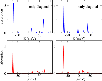
Figure 4: Normalized absorption spectrum $\alpha(\omega)$ for the non-resonant QD (left) and the resonant QD (right) at $T=77\,$K. The lower panels refer to the full model while the upper panels are restricted to level-diagonal phonon coupling. The bare h1$\rightarrow$e1 transition energy is chosen as zero of energy.

In Fig. 4, the absorption spectrum $\alpha(\omega)$ is shown for both the non-resonant QD (left) and the resonant one (right). In the lower panels, all phonon couplings are included. A set of closely spaced levels (bundle) is seen around the two main optically allowed exciton transitions h1-e1 and h2-e2. The excited-state bundle for the resonant QD exhibits a particular broad range. A simple theory like e.g. the second Born approximation KK98 would give here a real broadening of the line, which may be interpreted as a real dephasing process via energy-conserving phonon emission. We see that in the present exact treatment, the situation is a bit more complex, and can at best be called quasi-dephasing. Also, the comparison with the non-resonant dot (left) shows that quasi-dephasing is in no way restricted to exact resonance. Although a treatment of exciton occupation is outside the frame of the present paper, this finding points to the absence of a clear phonon bottleneck in polar quantum dots.

We have also calculated the spectrum for the reduced model of level-diagonal phonon coupling $M_{\mathbf{q}ij}^{a}\propto\delta_{ij}$ (upper panels in Fig. 4). This case is known to be exactly solvable and called Independent Boson Model, see Ref. Mahan . We found excellent agreement supporting our method, and could justify the chosen truncation in Boson occupation. The level-diagonal absorption spectrum exhibits phonon satellites which carry only a few percent of the total weight, leaving the zero phonon line as the dominant feature. The inclusion of the inter-level or non-adiabatic coupling thus changes the absorption spectrum significantly which was already emphasized in Ref. Fom98 .

In Fig. 5 we show the different contributions separately. Without Coulomb interaction (upper panel), the transitions are slightly shifted compared to their bare positions marked by dashed vertical lines. This allows to extract a polaron shift of the lowest transition in the non-resonant QD of 4 meV. This is much smaller than the standard expression for the polaron shift in bulk CdSe (electrons: 11.3 meV, holes: 21.1 meV) and shows indeed the strong charge cancellation in a QD as discussed in Ref. SMC87 . In addition, the restriction to a finite number of sublevels might underestimate our calculated QD polaron shift. The comparison with the full calculation including phonon and Coulomb interaction (middle panel) shows the importance of the exciton effect. There is a general shift which is related to the dominant diagonal Coulomb matrix element $v_{1111}=67.4$meV. However, the competition between nondiagonal Coulomb interaction and phonon coupling (which are of the same order of magnitude) modifies the spectrum in a complex manner, and cannot be reduced to a rigid spectral shift. This clearly shows the importance of excitonic effects in the absorption spectrum of strongly polar quantum dots.

In the lower panel, results of a calculation with only two hole levels are shown. The h3-e1 transition and its excitonic modification is, of course, missing here. Nevertheless, the basic features in the spectrum prevail. The polaron shift is a bit smaller and the spectrum is less “smeared out” compared to the full model with three hole levels (middle panel).

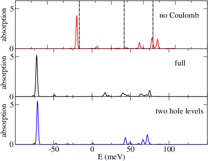
Figure 5: Normalized absorption spectrum $\alpha(\omega)$ for the non-resonant QD at $T=77\,$K. Upper panel: Without Coulomb interaction. The transition energies without phonon interaction are shown as vertical dashed lines which refer to the vertical arrows of Fig. 2. Middle panel: All couplings and levels included. Lower panel: Only two hole levels included.

V.2 Convolution approach

Performing the unitary transformation described in section III on the Hamiltonian for each band separately, we end up with a model containing three Bosonic modes for the conduction band and six Bosonic modes for the valence band. Using the conservation of the electron (hole) number and again a parabolic confinement potential, we finally have to diagonalize a Hamiltonian with two Bosonic modes and two Fermionic states for the conduction band and four Bosonic modes and three Fermionic states for the valence band. For the two-state model, this has been discussed at length in our previous paper Ref. SZC00 .

Within the convolution approach, excitonic effects can only be included approximately by a rigid shift of the spectrum using an ad-hoc exciton binding energy. In the following discussion, we want to demonstrate that even the electron-phonon interaction is not treated appropriately. Therefore, we have no Coulomb interaction in this subsection.

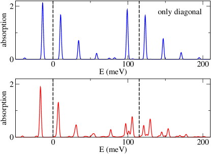
Figure 6: Normalized absorption spectrum $\alpha^{con}(\omega)$ obtained from convoluting the spectral functions for electron and hole in the non-resonant QD. The transition energies without phonon interaction are shown as vertical dashed lines. The upper panel refers to the diagonal phonon coupling, while the lower panel includes all coupling matrix elements.

In Figure 6, the absorption spectrum $\alpha^{con}(\omega)$ from the convolution of the spectral functions Eq. (27) is shown for the non-resonant case. In order to reach the same (artificial) broadening of the spectrum, we have to broaden the spectral functions with a Gaussian of reduced variance, $\sigma=1/\sqrt{2}\,$meV.

The inclusion of nondiagonal phonon matrix elements (lower panel) is not so important here, as the spectrum is dominated by strong phonon satellites. A comparison with the exact spectrum (neglecting excitonic effects) of Fig. 5 (upper panel) shows, however, that these satellites are much too strong. As discussed at the beginning of Sec. IV, it is the correlated phonon scattering between electron and hole states which reduces the satellite structure appreciably. Thus, the one-particle spectral functions are not able to describe the optical transitions properly. Thus, we conclude that the convolution approach as applied in Refs.KK98 ; VAM04 is insufficient, even if the phonon coupling is of moderate strength, as in the present example.

VI Summary

We have presented a solvable model which describes the optical properties of a single quantum dot interacting with LO phonons, and includes exciton formation. The linear polarization and the corresponding absorption spectrum is calculated by diagonalizing the appropriate Hilbert space of six electronic levels and six Bosonic modes split off from the full phonon modes via an orthogonalization procedure. The correct evaluation of the two-particle dipole-dipole correlation function is contrasted with a simplified approach using the spectral convolution of one-particle spectral functions. The numerics shows this convolution approach to be inadequate, as it gives phonon satellites strongly enhanced compared to the correct result. Qualitatively, this can be traced back to a missing compensation between different contributions in a diagrammatic analysis.

Parameter values for CdSe quantum dots are used, and a comparison between resonant and non-resonant QDs is carried out. Signatures of the phonon bottleneck are found, i.e. a stronger quasi-dephasing for the resonant case, but this is not as dramatic as simple arguments using Fermi’s golden rule for phonon emission would predict.

VII Acknowledgments

Funding from MCyT (Spain) through grant MAT2002-04095-C02-01 and from DFG (Germany) through Sfb 296 is acknowledged.

Appendix A Electron-Hole transformation

Switching from the conduction-valence-band description to the electron-hole picture produces a shift in the Bosonic operators. Here we show that only the shift of the zero-momentum mode survives.

To proceed we have to use the complete form of the confinement wave function including the Wannier basis $w_{a}({\bf r})$ of the band under consideration,

$$\Psi_{j}^{a}(\mathbf{r})=\sum_{\mathbf{R}}\psi_{j\mathbf{R}}^{a}\,w_{a}(\mathbf{r}-\mathbf{R})\,,$$ (33)

where $\psi_{j\mathbf{R}}^{a}$ is the envelope part (called confinement function in the previous sections). The orthogonality of the (real) wave functions induces

$$\delta_{jl}=\int_{\Omega}d^{3}r\,\Psi_{j}^{a}(\mathbf{r})\,\Psi_{l}^{a}(\mathbf{r})=\sum_{\bf R}\psi_{j\mathbf{R}}^{a}\,\psi_{l\mathbf{R}}^{a}\,,$$ (34)

since the Wannier functions are orthogonal on different lattice sites $\mathbf{R}\neq\mathbf{R}^{\prime}$. Dropping prefactors, we evaluate

$$\sum_{j}M_{\mathbf{q}jj}^{a} \propto \int_{\Omega}d^{3}r\,\sum_{\mathbf{R}\mathbf{R}^{\prime}j}\psi_{j\mathbf{R}}^{a}\,\psi_{j\mathbf{R}^{\prime}}^{a}\,e^{i\mathbf{q}\mathbf{r}}$$

$$\times w_{a}(\mathbf{r}-\mathbf{R})\,w_{a}(\mathbf{r}-\mathbf{R}^{\prime})\equiv C_{\mathbf{q}}\,.$$

The sum over $j$ gives a Kronecker symbol $\delta_{\mathbf{R}\mathbf{R}^{\prime}}$ due to the completeness of the coefficients $\psi_{j\mathbf{R}}^{a}$. The remaining integral simplifies to

$$C_{\mathbf{q}} = \int_{\Omega}d^{3}r\sum_{\mathbf{R}}e^{i\mathbf{q}\mathbf{r}}\,w_{a}^{2}(\mathbf{r}-\mathbf{R})$$

$$= \int_{\Omega}d^{3}r^{\prime}\,e^{i\mathbf{q}\mathbf{r}^{\prime}}\,w_{a}^{2}(\mathbf{r}^{\prime})\sum_{\mathbf{R}}e^{i\mathbf{q}\mathbf{R}}\,.$$

The last sum over $\mathbf{R}$ produces ${\cal N}\delta_{\mathbf{q}0}$, where ${\cal N}$ is the number of elementary cells $\Omega_{0}$ within the normalization volume, $\Omega={\cal N}\,\Omega_{0}$. Altogether we have

$$C_{\mathbf{q}}=\delta_{\mathbf{q}0}\,{\cal N}\,.$$ (37)

Therefore, the correction in the last line of Eq. (3) reduces to zero momentum,

$$\left(b_{0}^{\dagger}+b_{0}\right)\sqrt{{\cal N}\hbar\omega_{0}}\,\alpha_{v}(q)\,,$$ (38)

$$\alpha_{v}(q)=\sqrt{\frac{1}{\Omega_{0}}\frac{e^{2}}{2q^{2}\varepsilon_{0}}\left(\frac{1}{\varepsilon_{\infty}}-\frac{1}{\varepsilon_{S}}\right)}\,.$$

In the prefactor $\alpha_{v}(q)$, we let $q\to 0$ at the end.

In order to remove the last line from the Hamiltonian, the zero-momentum phonon operator is shifted according to

$$b_{0}+\alpha_{v}(q)\sqrt{{\cal N}/\hbar\omega_{0}}\rightarrow b_{0}\,,$$ (39)

which brings from the free phonon Hamiltonian a quadratic contribution ${\cal N}\alpha_{v}^{2}(q)$. Together with the valence energy sum, this gives an unimportant $c$ number contribution which can be dropped. However, the electron-phonon interaction is getting an addition at $\mathbf{q}\to 0$, too. Due to the orthogonality of the confinement functions, we have in leading order

$$M_{\mathbf{q}jl}^{a}=\sqrt{\frac{\hbar\omega_{0}}{\cal N}}\,\alpha_{v}(q)\left(\delta_{jl}+O(q)\right)\,,$$ (40)

which gives as correction

$$-2\alpha_{v}^{2}(q)\left(e_{i}^{\dagger}e_{i}\,-\,h_{i}^{\dagger}h_{i}\right)\,.$$ (41)

However, this term vanishes for any state having no or an equal number of electrons and holes (charge neutrality). For optical excitation and recombination, this is just the relevant sector of the Hilbert space. Therefore, the singularity in $\alpha_{v}(q)\propto 1/q$ (which would have to be treated carefully) does not contribute to physical quantities.

Finally, we note that the above argument also holds for acoustic phonons.

Appendix B Gram-Schmidt orthonormalization

We apply the Gram-Schmidt scheme by first constructing the orthogonal operator set

$$\tilde{B}_{1}=A_{1}\;,\quad\tilde{B}_{\lambda}=A_{\lambda}\,-\,\sum_{\alpha=1}^{\lambda-1}\left[A_{\lambda},B^{\dagger}_{\alpha}\right]B_{\alpha}\,,$$ (42)

and normalizing it afterwards via

$$B_{\lambda}=N_{\lambda}\tilde{B}_{\lambda}\quad\mbox{where}\quad N_{\lambda}^{-2}=\left[\tilde{B}_{\lambda},\tilde{B}_{\lambda}^{\dagger}\right]\,.$$ (43)

The new operators obey the canonical commutation rules

$$\left[B_{\lambda},B^{\dagger}_{\alpha}\right]=\delta_{\lambda\alpha}\,.$$ (44)

The final result can be written as a linear transformation

$$B_{\lambda}=N_{\lambda}\sum_{\alpha=1}^{\lambda}K_{\lambda\alpha}A_{\alpha}\,.$$ (45)

By construction, $K_{\lambda\alpha}$ is a tridiagonal matrix which has nonzero elements for $\lambda\geq\alpha$ only. The key ingredient for its evaluation is the commutator

$$\left[A_{\lambda},A^{\dagger}_{\alpha}\right] = \sum_{\mathbf{q}\,\mathbf{q}^{\prime}}M_{\mathbf{q}\lambda}M_{\mathbf{q}^{\prime}\alpha}^{*}\left[b_{\mathbf{q}},b^{\dagger}_{\mathbf{q}^{\prime}}\right]$$ (46)

$$= \sum_{\mathbf{q}}M_{\mathbf{q}\lambda}M_{\mathbf{q}\alpha}^{*}\equiv M_{\lambda\alpha}\,,$$

and we get a recursive determination according to

$$K_{\lambda\lambda} = 1\,,$$ (47)

$$K_{\lambda\alpha} = -\sum_{\beta=\alpha}^{\lambda-1}N_{\beta}^{2}K_{\beta\alpha}\sum_{\nu=1}^{\beta}M_{\lambda\nu}K_{\beta\nu}^{*}\quad(\lambda>\alpha)\,.$$

The norm follows from

$$N_{\lambda}^{-2}=\sum_{\alpha,\beta=1}^{\lambda}K_{\lambda\alpha}M_{\alpha\beta}K_{\lambda\beta}^{*}\,.$$ (48)

In order to transform the Hamilton operator to the new phonon operators $B_{\lambda}$, we need to invert Eq. (45),

$$A_{\lambda}=\sum_{\alpha=1}^{\lambda}I_{\lambda\alpha}B_{\alpha}\,.$$ (49)

Again, $I$ is tridiagonal and can be determined quite easily via

$$I_{\lambda\lambda}=1/N_{\lambda}\,,\quad\lambda>\alpha:\,I_{\lambda\alpha}=-\sum_{\beta=\alpha}^{\lambda-1}K_{\lambda\beta}I_{\beta\alpha}\,.$$ (50)

Appendix C Coupling matrix elements

The standard Fröhlich coupling for the electron-LO-phonon interaction is applied to the dot confinement states,

$$M_{\mathbf{q}jl}^{a} = \sqrt{\frac{\hbar\omega_{0}}{\Omega}\frac{e^{2}}{2q^{2}\varepsilon_{0}}\left(\frac{1}{\varepsilon_{\infty}}-\frac{1}{\varepsilon_{S}}\right)}\,\Phi_{\mathbf{q}jl}^{a}\,,$$ (51)

$$\Phi_{\mathbf{q}jl}^{a} = \int d^{3}r\,\psi_{j}^{a}({\mathbf{r}})\,e^{i\mathbf{q}\cdot\mathbf{r}}\,\psi_{l}^{a}({\mathbf{r}})\quad(a=c,v)\,.$$

In the subspace of one electron-hole pair states, the Coulomb interaction $H^{C}$ reduces to

$$\left<n_{\lambda},kl|H^{C}|n^{\prime}_{\lambda},ij\right>=-\delta_{n_{\lambda},n^{\prime}_{\lambda}}\,v_{klij}$$ (52)

which is diagonal in the phonon quantum numbers. The matrix element is given by

$$v_{klij} = \int\!d^{3}r\,d^{3}r^{\prime}\psi_{k}^{c}(\mathbf{r})\,\psi_{l}^{v}(\mathbf{r}^{\prime})\,\frac{e^{2}}{4\pi\varepsilon_{0}\varepsilon_{S}|\mathbf{r}-\mathbf{r}^{\prime}|}\,\psi_{j}^{v}(\mathbf{r}^{\prime})\,\psi_{i}^{c}(\mathbf{r})$$ (53)

$$= \frac{1}{\Omega}\sum_{\mathbf{q}}\Phi_{\mathbf{q}ki}^{c}\frac{e^{2}}{\varepsilon_{0}\varepsilon_{S}q^{2}}\Phi_{-\mathbf{q}lj}^{v}\,.$$

Diagonalizing the phonon-free part together with $H^{C}$ would lead to (non-polar) exciton transition energies. However, in the present context it is more appropriate (and easier) to diagonalize phonon and excitonic effects together. Consequently, the main interband transition energies are related to exciton-polaron states in the quantum dot.

For simplicity we consider an anisotropic parabolic potential as dot confinement for both, electrons and holes, with $x$ as the long axis. The three energetically lowest wave functions are given by

$$\psi_{1}^{a}(\mathbf{r}) = \frac{1}{N_{a}}\exp-\frac{1}{2}\left(\frac{x^{2}}{X_{a}^{2}}+\frac{y^{2}}{Y_{a}^{2}}+\frac{z^{2}}{Z_{a}^{2}}\right)\,,$$

$$\psi_{2}^{a}(\mathbf{r}) = \sqrt{2}\frac{x}{X_{a}}\psi_{1}^{a}(\mathbf{r})\,,$$ (54)

$$\psi_{3}^{a}(\mathbf{r}) = \left(\sqrt{2}\frac{x^{2}}{X_{a}^{2}}-\frac{1}{\sqrt{2}}\right)\psi_{1}^{a}(\mathbf{r})\;,$$

where $X_{a}>Y_{a},Z_{a}$ are the spatial extensions (variances) of the ground state, and $N_{a}^{2}=\pi^{3/2}X_{a}Y_{a}Z_{a}$ its normalization.

The matrix elements in Eq. (51) and Eq. (53) thus read

$$\Phi_{\mathbf{q}11}^{a} = \exp\left(-\frac{1}{4}\left(q_{x}^{2}X_{a}^{2}+q_{y}^{2}Y_{a}^{2}+q_{z}^{2}Z_{a}^{2}\right)\right)\,,$$

$$\Phi_{\mathbf{q}21}^{a} = iq_{x}X_{a}/\sqrt{2}\,\Phi_{\mathbf{q}11}^{a}\,,$$

$$\Phi_{\mathbf{q}31}^{a} = -q_{x}^{2}X_{a}^{2}/\sqrt{8}\,\Phi_{\mathbf{q}11}^{a}\,,$$

$$\Phi_{\mathbf{q}22}^{a} = \left(1-q_{x}^{2}X_{a}^{2}/2\right)\Phi_{\mathbf{q}11}^{a}\,,$$ (55)

$$\Phi_{\mathbf{q}32}^{a} = i\left(q_{x}X_{a}-q_{x}^{3}X_{a}^{3}/4\right)\Phi_{\mathbf{q}11}^{a}\,,$$

$$\Phi_{\mathbf{q}33}^{a} = \left(1-q_{x}^{2}X_{a}^{2}+q_{x}^{4}X_{a}^{4}/8\right)\Phi_{\mathbf{q}11}^{a}\;.$$

Notice that $\Phi_{\mathbf{q}22}^{v}=\Phi_{\mathbf{q}11}^{v}+\Phi_{\mathbf{q}31}^{v}/\sqrt{2}$. Therefore, one additional Bosonic mode can be eliminated.

The new coupling constants $M_{\lambda\alpha}$ are obtained by integrating a pair of coupling constants $M_{\mathbf{q}ij}^{a}$ over $\mathbf{q}$, Eq. (46). This final integration can be reduced to the following (elliptic) integrals,

$$J_{n}=\int_{1}^{\infty}dt\,\frac{t^{-n}}{\sqrt{t(t-p)(t-q)}}\quad(n=0,1,2,3,4)$$ (56)

with $p=1-(Y_{a}^{2}+Y_{b}^{2})/(X_{a}^{2}+X_{b}^{2})<1$ and $q=1-(Z_{a}^{2}+Z_{b}^{2})/(X_{a}^{2}+X_{b}^{2})<1$. For a cylindrically symmetric potential with $Y_{a}=Z_{a}$, we have $p=q$, and the integrals reduce to simple analytic functions,

$$J_{0}=\frac{1}{\sqrt{p}}\log\frac{1+\sqrt{p}}{1-\sqrt{p}}\,,\quad J_{n+1}=\frac{J_{n}-(n+1/2)^{-1}}{p}\,.$$ (57)

The same type of integration over $\mathbf{q}$ appears in the Coulomb matrix elements Eq. (53). For example, the diagonal matrix element for the lowest transition h1-e1 can be evaluated as

$$v_{1111}=\frac{e^{2}}{\varepsilon_{0}\varepsilon_{S}\sqrt{X_{c}^{2}+X_{v}^{2}}}\,\frac{J_{n=0}}{4\pi^{3/2}}$$ (58)

where $p$ and $q$ in Eq. (56) are determined with $a=c,\,b=v$.

Appendix D Material parameters

Parameter values for the polar semiconductor material CdSe forming the quantum dot are from Ref. Puls99 as LO-phonon energy $\hbar\omega_{0}=24\,$meV, conduction band mass $m_{c}=0.13\,m_{0}$, and valence band mass $m_{v}=0.45\,m_{0}$. Dielectric constants have been taken from Ref. LanBoer : $\varepsilon_{S}=9.57$, $\varepsilon_{\infty}=6.27$.

We assume that the confinement potentials of electrons and holes are scaled by a fixed ratio $\rho$ which equals the ratio between conduction band offset and valence band offset for barrier (ZnSe) and dot material (CdSe), $\rho=5.44$ Puls99 . Applying this to the parabolic potential, we find a unique ratio between the lengths in the oscillator eigenfunctions Eq. (C),

$$\xi\equiv\frac{L_{c}}{L_{v}}=\left(\frac{m_{v}}{m_{c}\rho}\right)^{1/4}\,,\quad(L=X,Y,Z)$$ (59)

which equals $\xi=0.89$.

Since the $x$ direction is taken as the longest one, the energetic distance between ground level ($j=1$) and first excited level ($j=2$) is exclusively given by the $x$-confinement,

$$\Delta^{a}\equiv|\epsilon_{2}^{a}-\epsilon_{1}^{a}|=\frac{\hbar^{2}}{m_{a}X_{a}^{2}}\quad(a=c,v)\,.$$ (60)

Taking experimental values which have been reported for a certain CdSe quantum dot in Refs. FlissHen01 ; Akimov04 ($\Delta^{c}=80\,$meV, $\Delta^{v}=35\,$meV) we obtain according to Eq. (60) $X_{c}=2.71\,$nm and $X_{v}=2.20\,$nm. This yields a length ratio of $\xi=X_{c}/X_{v}=1.23$ which is larger than the value derived from Eq. (59). However, a possible alloying of the QD material GKFNZGT04 and deviations from the (idealized) parabolic confinement potential may introduce substantial uncertainties. In the numerical calculations, we have used $\xi=1.23$ throughout.

There is no direct experimental access to the size of the QD in the other (shorter) directions. To keep things simple, we take the same representative value for the two smaller lengths: $Y_{v}=Z_{v}=1.3\,$nm and $Y_{c}=Z_{c}=\xi Y_{v}=1.6\,$nm. The next levels corresponding to this shorter length would have a spacing of $100\,$meV in the valence band. Since this is larger than twice the level spacing corresponding to the larger $X$ extension ($70\,$meV), we have properly selected the lowest hole confinement states in Eq. (C).

It is easily seen from the parity of the oscillator wave functions Eq. (C), that the optical transitions h1$\rightarrow$e2, h2$\rightarrow$e1 and h3$\rightarrow$e2 are forbidden. The remaining non-zero dipole matrix elements Eq. (18) can be expressed by the same length ratio $\xi$ introduced above. In units of $\mu_{cv}$, we find

$$\mu_{11} = \left(\frac{2\xi}{1+\xi^{2}}\right)^{1/2}\,,\quad\mu_{22}=\left(\frac{2\xi}{1+\xi^{2}}\right)^{3/2}\,,$$

$$\mu_{31} = -\left(\frac{\xi}{1+\xi^{2}}\right)^{1/2}\frac{1-\xi^{2}}{1+\xi^{2}}\,.$$ (61)

With $\xi=1.23$, we get $\mu_{11}=0.99$, $\mu_{22}=0.97$ and $\mu_{31}=0.14$. Such values very close to a Kronecker delta are typical for the strong confinement in a quantum dot. The energetic distance between the dominant transitions equals $\Delta^{c}+\Delta^{v}=115\,$meV (without polaron and Coulomb corrections).

Apart from the parameter set deduced from the experimentally given level distances, we chose another one which has perfect resonance between the hole level distance and the LO phonon energy, i.e. $\Delta^{v}=24\,$meV. This yields a somewhat larger QD with $X_{v}=2.66\,$nm and $X_{c}=\xi X_{v}=3.27\,$nm, while keeping all the other parameters the same. The level distance for the electrons amounts to be $\Delta^{c}=55\,$meV, giving an energetic distance between the main allowed transitions of 79 meV. We call this the resonant QD, while the parameter set backed by experiment is referred to as the non-resonant QD.

The diagonal Coulomb matrix elements are in the range of 50-70 meV which is four times the exciton binding energy in bulk CdSe (15 meV) and quantifies the strong enhancement of Coulomb effects in small QDs. The non-diagonal Coulomb matrix elements are around 15 meV which is comparable to the effective phonon coupling strengths.

References

- (1) L. Bányai and S. W. Koch, Semiconductor Quantum Dots (World Scientific, Singapore, 1993).
- (2) M. G. Bawendi, P. J. Carroll, W. L. Wilson, and L. E. Brus, J. Chem. Phys. 96, 946 (1992).
- (3) J.R. Guest, T. H. Stievater, X. Li, J. Cheng, D. G. Steel, D. Gammon, D. S. Katzer, D. Park, C. Ell, A. Thranhardt, G. Khitrova, and H.M. Gibbs, Phys. Rev. B 65, 241310(R) (2002).
- (4) T. Flissikowski, A. Hundt, M. Lowisch, M. Rabe, and F. Henneberger, Phys. Rev. Lett. 86, 3172 (2001).
- (5) L. Jacak, J. Krasnyj, W. Jacak, R. Gonczarek, and P. Machnikowski, Phys. Rev. B 72, 245309 (2005).
- (6) U. Bockelmann and G. Bastard, Phys. Rev. B 42, 8947 (1990).
- (7) S. Schmitt-Rink, D. A. B. Miller, and D. S. Chemla, Phys. Rev. B 35, 8113 (1987).
- (8) O. Verzelen, R. Ferreira, and G. Bastard, Phys. Rev. Lett. 88, 146803 (2002).
- (9) L. Besombes, K. Kheng, L. Marsal, and H. Mariette, Phys. Rev. B 63, 155307 (2001).
- (10) A. Vagov, V.M. Axt and T. Kuhn, Phys. Rev. B 66, 165312 (2002).
- (11) E.A. Muljarov and R. Zimmermann, Phys. Rev. Lett. 93, 237401 (2004).
- (12) K. Král and Z. Khás, Phys. Rev. B 57, R2061 (1998).
- (13) T. Stauber, R. Zimmermann, and H. Castella, Phys. Rev. B 62, 7336 (2000).
- (14) L. Jacak, J. Krasnyj, D. Jacak, and P. Machnikowski, Phys. Rev. B 67 035303 (2003).
- (15) V. M. Fomin, V. N. Gladilin, J. T. Devreese, E. P. Pokatilov, S. N. Balaban, and S. N. Klimin, Phys. Rev. B 57, 2415 (1998).
- (16) L. Jacak, P. Machnikowski, J. Krasnyj, and P. Zoller, Eur. Phys. J. D 22, 319 (2003).
- (17) V. López-Richard, S. S. Oliveira, and G.-Q. Hai, Phys. Rev. B 71, 075329 (2005).
- (18) M. I. Vasilevskiy and E. V. Anda, and S. S. Makler, Phys. Rev. B 70, 035318 (2004); M.I. Vasilevskiy, R.P. Miranda, E.V. Anda, and S.S. Makler, Semicond. Sci. Technol. 19, S312 (2004).
- (19) R. Zimmermann and E. Runge, in Proc. 26th ICPS, Edinburgh (Inst. of Physics Publ., 2002).
- (20) Y. Gu, I.L. Kuskovsky, J. Fung, G.F. Neumark, X. Zhou, S. P. Guo, and M.C. Tamargo, phys. stat. sol. (c) 1, 779 (2004).
- (21) M. Reed and B. Simon, Methods of Modern Mathematical Physics I (Academic Press, New York, 1975).
- (22) I.A. Akimov, T. Flissikowski, A. Hundt, and F. Henneberger, phys. stat. sol. (a) 201, 412 (2004).
- (23) B. Krummheuer, V. M. Axt, and T. Kuhn, Phys. Rev. B 65, 195313 (2002).
- (24) P. Machnikowski and L. Jacak, Phys. Rev. B 71, 115309 (2005).
- (25) G.D. Mahan, Many-Particle Physics (Plenum Press, New York, 1990).
- (26) J. Puls, M. Rabe, H.-J. Wünsche, and F. Henneberger, Phys. Rev. B 60, R16303 (1999).
- (27) O. Madelung, ed., Semiconductors (Springer, Berlin, 1986), Landolt-Boernstein New Series.