Noise properties of two single electron transistors coupled by a nanomechanical resonator
Abstract
We analyze the noise properties of two single electron transistors (SETs) coupled via a shared voltage gate consisting of a nanomechanical resonator. Working in the regime where the resonator can be treated as a classical system, we find that the SETs act on the resonator like two independent heat baths. The coupling to the resonator generates positive correlations in the currents flowing through each of the SETs as well as between the two currents. In the regime where the dynamics of the resonator is dominated by the back-action of the SETs, these positive correlations can lead to parametrically large enhancements of the low frequency current noise. These noise properties can be understood in terms of the effects on the SET currents of fluctuations in the state of a resonator in thermal equilibrium which persist for times of order the resonator damping time.
I Introduction
Nanoelectromechanical systems in which micron-sized mechanical resonators couple to the transport electrons of a nearby conductor form a new and interesting class of mesoscopic system.nems In particular, there has been considerable theoreticalwhite ; mmh ; ABZ ; ADA ; bruder ; Clerk1 ; Clerk2 ; blencowe and experimentalmset1 ; mset2 interest in the properties of nanomechanical single electron transistors in which a mechanical resonator forms the voltage gate of the transistor. For these systems, the conductance properties of the SET are extremely sensitive to the resonator motion and such a device has been used to measure the displacement of a nanomechanical resonator with almost quantum limited precision.mset2
Apart from its application as an ultra-sensitive displacement detector, the SET-resonator system has a number of interesting features arising from its coupled dynamics. As electrons pass through the island of the SET they exert a stochastic driving force on the resonator, but the motion of the resonator in turn affects the rates at which electrons tunnel between the leads and the island of the SET, leading to non-trivial correlations between the electrical and mechanical motion. In general the resonator-SET system has a complicated coupled dynamics, but in the experimentally relevant regime of relatively large applied bias, but low electromechanical coupling and resonator frequency, the effect of the electrons on the mechanical resonator turns out to be closely analogous to that of an equilibrium thermal bath.ABZ ; blencowe
The correlations between the electrical and mechanical degrees of freedom in nanomechanical SETs also give rise to a number of unusual features in the current noise spectrum of the SET. There is a strong enhancement of the current noise at the resonator frequency, there can also be a strong enhancement at the first harmonic of the resonator frequency and at low frequencies.ADA Similar features have also been predicted in the noise spectra of a number of closely related nanoelectromechanical systems.isac ; bruder ; novotny ; Clerk1 ; Clerk2 Of particular interest in such systems is the unusual behavior of the zero-frequency current noise, which can become parametrically large when the resonator is under damped.isac ; novotny
Enhancement of the zero-frequency current noise is also known to occur, under certain circumstances, in systems consisting of two parallel SETs, or quantum dots, with a direct electrostatic interaction between the two islands. Such systems have been investigated quite extensively,set1 ; set2 ; set3 ; qd1 and it has been shown that the electrostatic interactions between charges on the two island give rise to important cross-correlations between the currents in the individual SETsset1 which can generate either positive or negative correlations between the carriers and hence either enhance or suppress the noise, depending on the exact details of the system.set1 ; set2 ; set3 ; qd1 Apart from their intrinsic interest, correlations between the currents of two SETs can be used to enhance the sensitivity of charge detection.buehler
In this paper we investigate the noise properties of a system consisting of a nanomechanical resonator coupled to two SETs aligned in parallel and relate them to the dynamics of the resonator. The resonator is assumed to lie between the islands of the two SETs acting as a mechanically compliant voltage gate for both of them. In order to act as a gate, the resonator is coated with a thin metal layer and kept at a fixed voltage. Under such circumstances there is no direct electrostatic interaction between the SET islands, but the mutual interaction between the electrons travelling through the SETs and the resonator nevertheless generates correlations between the currents flowing in the two conductors.
As electrons pass through the SETs they exert a stochastic force on the resonator which can strongly affect its motion, but the motion of the resonator in turn affects the motion of electrons through the SETs. We find that the dynamical state of a resonator coupled to two SETs is approximately equivalent to that of an oscillator coupled to two independent thermal baths. We also find that the presence of the resonator strongly enhances the low frequency current noise of the individual SETs and generates positive correlations between the currents in the two SETs. The correlations in the currents within each of the individual SETs, and between the currents in the two SETs, are generated by fluctuations in the state of the resonator and hence the magnitude of the low frequency noise depends sensitively on the time-scale over which they decay, the damping time of the resonator. Although the fluctuations in the state of the resonator are in turn generated by the motion of the electrons through the SETs, the resulting noise properties are very similar to those obtained if the back-action of the SETs on the resonator is neglected and instead the resonator is assumed to be in a fixed thermal state with appropriately chosen parameters.
The outline of this paper is as follows. In Section II we describe our model for the two-SET resonator system and the conditions under which it is valid. We also introduce the master equation formalism which is used to derive the subsequent results. Then in Section III we analyze the dynamics of the resonator when coupled to two SETs and compare the results to those obtained for a resonator coupled to a single SET. In Section IV we investigate the noise properties of the SET currents. First, we present calculations of the zero-frequency current noise in one of the SETs and relate the results to a simple model where the back-action of the SETs on the resonator is neglected. Then we describe the cross-correlations between the currents in the two SETs, and how they can be investigated via measurements on the combined currents through the two leads. Finally, in Section V we present our conclusions. The Appendix contains additional details about how an effective equation for the resonator is derived.
II Model System
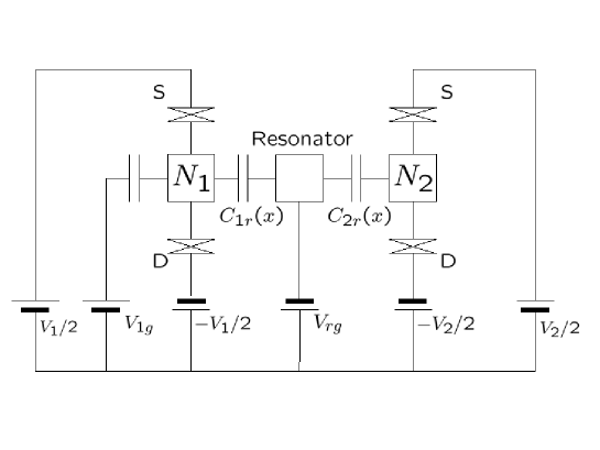
The system of two SETs coupled to a nanomechanical resonator which we consider is illustrated schematically in Fig. 1. The SET islands, labelled 1 and 2, are linked to voltage leads by source (S) and drain (D) junctions across which voltages and respectively are applied. The resonator acts as a movable gate for island 1(2) with capacitance which depends on its position, . In practice the motion of the resonator will be very small on the scale of the equilibrium separation between it and the SET islands, , and hence can be treated as a linear perturbation, . We also assume that SET 1 has an additional gate with a capacitance and voltage so that the operating points of the two SETs can be tuned independently.
The dynamics of the system can be described using a generalization of the classical master equation formalism which was used to analyze the coupled dynamics of a nanomechanical resonator coupled to one SET.ABZ ; ADA The basic assumptions underlying this approach are that the charge state of the SET islands are each limited to two possible values by charging effects, with transitions between these charge states occurring via electron tunnelling processes which are adequately described by the orthodox model,ferry and that the resonator can be treated as a classical harmonic oscillator. These conditions are met if the background temperature is much lower than the charging energy of the SET islands, the SETs are assumed to tuned to, or close to, degeneracy and the drain-source voltages applied are much larger than the quantum of energy associated with the resonator.ABZ
Since the electronic motion is stochastic, the system may be described by a set of probability distributions of the form , which give the probability at time of having excess electrons on the island of SET 1, excess electrons on the island of SET 2 and the resonator being at a position with velocity . The superscripts on the distributions, , are count variables which give the number of electrons that have passed through the source junction of SET 1(2). Although the count variables have no effect on the resonator dynamics, they play an important role in the analysis of the noise properties of the SETs.
The resonator is assumed to be a simple harmonic oscillator with frequency and effective mass . The quantum of energy associated with the resonator, , is assumed to be the smallest energy in the problem, so that it is always much less than the energies associated with the voltages applied across the SET islands, and , to ensure that quantum effects in the resonator’s dynamics can be neglected. The relevant charge states for the SETs are assumed to have and excess electrons on island . We choose the origin of resonator position such that is the equilibrium position of the resonator (i.e. the minimum in its potential) when there are and electrons on SET islands 1 and 2, respectively. If there are electrons on island 1(2), the equilibrium position of the resonator is shifted by the electrostatic force to , and if both islands contain an extra electron, then the equilibrium position of the resonator is shifted by . The lengths and are essentially measures of the strength of the interaction between the SETs and the resonator, they are given by where is the total capacitance of SET island 1(2) and is the separation between between SET island 1(2) and the resonator measured along the direction of increasing (hence the signs of and will be opposite for the setup in Fig. 1).
Transitions between the charge states of the SET islands are described by the rates for electron tunnelling forwards (positive charge moving from source to drain), , or backwards, , through the source (drain) tunnel junctions of islands or , which are written as and . According to the orthodox model,ferry these electron tunnelling rates depend on the differences in electrostatic energy of the system before and after the tunnelling events. The resonator affects the tunnel rates because its motion changes the gate capacitance of the SET islands and hence the electrostatic energy differences. Assuming that the thermal energies of the electrons in the SETs, and the energies associated with the electromechanical couplings, , are both much less than the energy scale set by the voltages, , then the backward tunnel rates can be set to zero and the forward tunnel rates can be written in an intuitive way asABZ ; ADA
| (1) | |||||
| (2) |
where are the position-independent parts of the tunnel rates, and is the resistance of the relevant SET tunnel junction. Notice that we have assumed that the coupling is weak enough that it can be treated linearly.ABZ
We are now in a position to set up the master equations for the system. However, the overall number of parameters describing the system remains rather large, making it difficult to extract the essential features of the dynamics. Hence, we will make a few further simplifying assumptions. We choose to consider only the case where the couplings of the SETs to the resonator are equal and opposite, , and we assume that the resistances of all the tunnel junctions have the same value, . Finally, we assume that the SETs are tuned to the current peaks through the gate voltages so that the position independent parts of the tunnelling rates through the source and drain junctions of each SET are equal. As long as the charging energies are larger than the voltages (), the orthodox model predicts tunnel rates at the current peak which are proportional to the source-drain voltages:korotkov_94 ; korotkov_96 .
The most obvious way to describe how the state of the system evolves would be to derive master equations for the four distributions , , and . However, in practice it proves more convenient to work with an alternative set of distributions composed of
| (3) | |||||
| (4) | |||||
| (5) |
and . These distributions are found to evolve according to the following set of master equations, written in dimensionless form:
| (6) | |||||
| (7) | |||||
| (8) | |||||
| (9) | |||||
where position and time have been scaled by and respectively, with the average voltage introduced to preserve the natural symmetry of the equations. The dimensionless electromechanical coupling is given by , the resonator frequency is expressed in dimensionless units as , and the dimensionless tunnel rates, , are defined by the relations: and .
The coupled set of master equations contain all the information about the dynamics of the system and can be used to extract information both about the motion of the resonator and about the noise properties of the SETs. In exploring the behavior of the system we will concentrate on the effects of varying three parameters: the reduced frequency of the resonator, , the electromechanical coupling and the ratio of SET voltages (which also changes ). However, because of the underlying assumptions in the model these parameters cannot be varied arbitrarily. In particular, the range of values for the voltages and is bounded below, and the strength of the electromechanical coupling is bounded above, by the requirement that the energy changes involved in electron tunnelling are dominated by the SET bias voltages rather then the position dependent correction, i.e. , or equivalently . The range of values of bias voltages is bounded above by the requirement that the number of accessible charge states for each SET should be limited to two, which essentially means that the charging energy of the SET islands should be the largest energy-scales in the problem, i.e. . In what follows, when we discuss variations in the system parameters, we will implicitly be assuming that the variation is always within the range discussed. For example, when we consider the case where , we nevertheless assume that .
III Resonator Dynamics
The dynamics of the resonator is governed by the evolution of the probability distribution . The equation of motion for forms part of an apparently complex set of four coupled equations [Eqs. (6)-(9)]. However, equations of motion for moments of the resonator’s probability distribution are readily obtained from the master equations. Furthermore, the master equations can be solved numerically using the techniques described in Ref. [ABZ, ].
The behavior of the first moments of the resonator are described by a set of four coupled differential equations:
| (10) | |||||
| (11) | |||||
| (12) | |||||
| (13) |
where the electron-resonator moments are defined using the notation
| (14) | |||||
| (15) |
The full solution of this set of equations offers little insight, but if we make some approximations based on the realistic assumption that the resonator frequency is much lower than the electronic tunnelling rate (i.e. ), then a simple equation of motion for the average position of the resonator about its fixed point can be derived:
| (16) |
as discussed in the Appendix. It is clear that the resulting equation of motion for the average position of the resonator is essentially just that of a damped harmonic oscillator with a shifted frequency, , and a damping constant , where .
The form of the equation of motion for strongly suggests that the resonator will have a well-defined steady state, and indeed this is what is found when the master equations [Eqs. (6)-(9)] are integrated numerically. Furthermore, numerical integration also reveals that for the steady state probability distribution is very well approximated by a Gaussian, something that is readily verified by calculating the steady state values for higher moments of the resonator. Thus we can characterize the steady state of the resonator by the variances in the position and velocity, and .
We can calculate equations of motion for the second moments in a similar way to that employed in Ref. ABZ, . For example the equation of motion for is obtained by by multiplying Eq. (6) by and then integrating over and in the the same way as for the first moments. Setting the rate of change of the second order moments to zero (i.e. etc.) leads to a coupled set of algebraic equations for the steady state values of the second moments. For , we find that the variances and obey equipartition. When we are also in the weak coupling limit () the variances (in dimensionful units) are
| (17) |
where . Bearing in mind that if only SET 1(2) were present the system would (in this weak coupling limit) have an effective temperature of the formABZ , we can rewrite the variances in terms of an effective temperature which is an average of the effective temperatures associated with each of the SETs:
| (18) |
where . These results show that in the weak-coupling limit the effective temperature and damping constant for the resonator coupled to two SETs take exactly the same form as those obtained previously for a resonator coupled to one SET and an external heat bath, characterized by its own temperature and damping constant.ABZ Thus for the two-SET resonator system we can think of each of the two SETs as acting on the resonator as an independent heat bath.
For the particular case when the two SETs are identical (i.e. ), then the ratio of the variances of the resonator position when coupled to just one of the SETs, , to that when it is coupled to both SETs, , takes the form
| (19) |
For it seems that adding a second SET (identical to the one already coupled to the resonator) has almost no effect on the resonator’s state. However, although the variances of the resonator are almost unaffected by adding (or removing) an identical SET, the value of the damping due to the SET electrons doubles when a second SET is added.
In practice the dynamics of a nanomechanical resonator would also be affected by thermal fluctuations arising from its surroundings which can be characterized by a temperature, and damping constant, . However, in what follows we will assume that the dynamics of the resonator is dominated by the SET back-action so that and and hence neglect the effects of these additional fluctuations on the SET noise characteristics. This back-action dominated regime is expected to be accessible experimentally for resonators with lengths m or longer, as discussed in Ref. ABZ, .
IV Noise Properties
Motion of the resonator affects the tunnel rates of the electrons in both the SETs and hence can induce correlations not just in the current flowing in the individual SETs, but also between the currents in the two SETs, known as auto- and cross-correlations respectively. The power spectrum of the auto-correlation function gives the current noise in one of the SETs, while the current noise of the combined currents of the two SETs are given by a combination of the power spectra of the auto- and cross-correlations. We begin this section by outlining how the zero frequency current noise in one of the SETs of the two-SET resonator system can be obtained. Then we analyze the noise in one of two SETs coupled to a resonator, and compare it with the noise in a single SET coupled to a resonator which is held in a fixed thermal state rather than one determined by the back-action of the SETs. Finally we examine the cross-correlations in the currents of the two SETs induced by being coupled to a resonator, and hence calculate the noise in their combined current.
IV.1 Current noise in one SET
The zero frequency current noise of SET 1, , is equal to the noise in the tunnel current across either of its junctions. Considering the source junction for concreteness, we havegurvitz
| (20) |
where
and we have used a result due to MacDonaldmac to rewrite the current through the source junction, , in terms of the number of charges that have passed through that junction.gurvitz Substituting for the rates of change of the distributions from the master equations [Eqs. (6)–(9)], we can rewrite the expression for the noise, in units of time where , as:
| (21) |
The calculation of the zero frequency noise thus reduces to the calculation of the limiting behavior of two electron-resonator moments. The long time limits of the moments are readily obtained analytically using an extension of the equation of motion method discussed in Ref. ADA, . Substituting these values for the moments into Eq. (21), gives an expression for the zero-frequency current noise. However, the resulting expression is hard to interpret. Hence in order to obtain a more accessible expression, we expand in the coupling parameter and then make the simplifying assumption . Up to order , the resulting expansion is:
| (22) |
where we have scaled the noise by , the average current of the SET without coupling to the resonator. The first term in the expansion, , is just the Fano factor of SET 1 (which in this case has equal tunnel rates across both junctions) in the non-interacting limit. The expansion is compared with the full analytical expression in Fig. 2; the agreement is very good for as one would expect.
The presence of the resonator affects the current noise because fluctuations in its motion, caused by interactions with the electrons in either SET, generate correlations in the current. The expansion in terms of shows clearly that the current noise increases with increasing coupling, measured by . However, the expansion also shows that the noise is extremely sensitive to the value of , diverging in the limit . The explanation for this behavior is that the zero frequency current noise is controlled by the fluctuations in the state of the resonator which decay on a time-scale of order the damping time, . This damping time is determined by the back-action, and also diverges in the limit . The fact that the intrinsic damping of the resonator, , vanishes as means the fluctuations do not decay and therefore the current noise diverges. This idea can be tested directly by comparing the current noise of the two-SET resonator system with that of a SET coupled to a resonator whose damping (and temperature) is determined solely by coupling to an external thermal bath (i.e. the back-action of the SETs on the resonator is neglected).
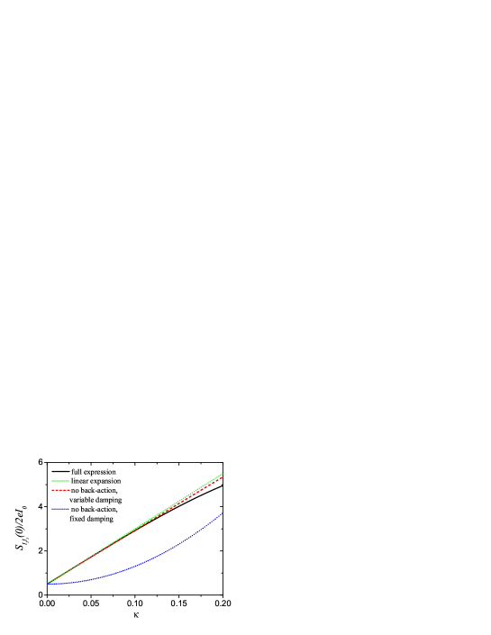
The back-action of the SET on the resonator arises from the displacement of the equilibrium position of the resonator caused by changes in the occupancy of the SET islands. When these displacements are neglected, the motion of the resonator can still affect the electron tunnelling rates of the SET, but the resonator is no longer affected by the electrons. We calculate the zero frequency noise in the same way as before but without the back-action terms, instead assuming that the resonator is coupled to an external equilibrium thermal bath, characterized by a temperature and a damping constant, . With all other parameters held constant, the current noise diverges as , showing that the divergence in the current noise is indeed due to the damping going to zero.blanter
The noise obtained for the fully coupled system and the no back-action model are compared in Fig. 2. Two particular choices of parameters for the external bath are shown: one with a fixed value of the bath damping, , and one with chosen to match the dependent effective value of the equivalent fully coupled case (i.e. ). In both cases, we choose the temperature of the bath to match the small-coupling value of the equivalent fully coupled case (i.e. we set , which is independent of ). The noise for the no back-action case is almost linear in when the value of is varied to match that of the equivalent fully coupled case, but only has a small linear term when instead is kept constant. This shows that in the fully coupled case, it is the fact that the damping depends on that gives a linear (rather than ) dependence of the current noise.
IV.2 Current cross-correlations
Having analyzed the zero-frequency current noise of one of the SETs in the two-SET resonator system, we now turn to consider the correlations between the currents in the two SETs induced by the presence of the resonator. The cross-correlation between the two SETs is defined as
| (23) |
where , and the correlation function is assumed to be independent of . The power spectrum of the cross-correlation is defined as,
| (24) |
The zero frequency limit is independent of whether we consider cross-correlations in the full currents flowing through the SETs or in the tunnel currents across either the source or drain junctions, and is given by
| (25) | |||||
| (26) |
where we have used a generalization of MacDonald’s formula in the last line to recast the expression into a form which is readily evaluated using the generalized master equations. Substituting appropriately from the master equations [Eqs. (6)-(9)] for the rates of change of the probability distributions, we obtain
The moments () and () describe the correlations between the resonator, the charge on SET 2 (1) and the charge that has passed through SET 1 (2). They are readily obtained using the same equation of motion approach employed for the single-SET moments.
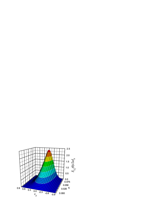
The cross-correlation noise, is shown in Fig. 3 as a function of the parameters and , which measures the difference between the voltages. It is clear from the plot that the cross-correlations are positive, reaching a maximum when the two voltages are equal and increasing with the coupling, .
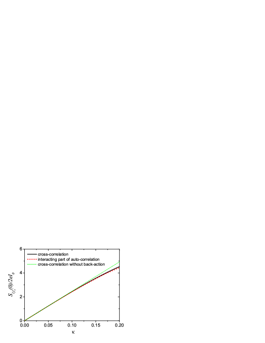
In order to understand the cross-correlation, we can again make a comparison with the case of a resonator in a fixed thermal state where the back-action of the electrons on the resonator is neglected. Without the back-action, with the state of the resonator controlled by coupling to an external equilibrium thermal bath, there is no way for the electrons in the two SETs to influence each other as they cannot affect the state of the resonator. The zero frequency component of the cross correlation with and without the back-action are compared in Fig. 4, where the temperature and damping associated with the external bath for the no back-action case have been chosen to match those of the fully coupled system, and it is clear that they coincide up to linear order in . We can think of the electrons in both SETs acting on the resonator to form a dynamical state which then acts back on the electrons in both SETs to induce correlations. When the back-action of the electrons on the resonator is neglected, and it is kept in a thermal state by an external bath, correlations are still induced between the SETs because both SETs experience the same fluctuations in the resonator’s state. Fig. 4 also compares the zero frequency component of the cross-correlation with the corresponding part of the auto-correlation which arises from interactions with the resonator, [See Eq. (22)], for identical SETs (i.e. ). It is clear from Fig. 4 that and are closely related even for values of which approach the limit of the model’s validity and indeed we find that in the limit they become equal.
These results are at first a little surprising as the cross-correlations between carriers in different leads of a device are very often negative. Indeed, so long as the voltages applied are constant and there are no interactions the cross-correlations must be negative.buttiker_92 ; bandb ; cottet_04 However, in our system although the leads are kept at fixed voltages and contain non-interacting electrons, the presence of the resonator generates effective interactions within the device itself (i.e. between the islands of the SETs) and hence positive correlations between currents in different leads are possible. Positive current-correlations between leads were also found for similar systems consisting of parallel quantum dots with a direct electrostatic interaction between them.set1 ; note
We might also expect the cross-correlations to be negative because the signs of the SET-resonator coupling terms are opposite so that when the resonator moves towards SET 1 (effectively decreasing the tunnelling rate ) it moves away from SET 2 (increasing ). However, we must remember that the correlations are between and in the limit , i.e. all motions of the resonator are averaged out over a long time. The two SETs experience the same fluctuations in the state of the resonator and hence, provided the SETs are identical, these fluctuations induce essentially the same correlations between the currents of the two SETs as within the current of each one separately. However, this will not be the case at finite frequency. In particular, we would expect strong anti-correlation between the currents in the two SETs at the resonator frequency.
A simple way to measure the cross-correlations in the currents through the two SETs is to measure the noise in the combined current of the two SETs, , and compare the result with the noise in the currents through the individual SETs, and . The zero frequency noise of the combined current is given by
| (27) |
Thus measuring the noise in the combined current of the SETs and comparing it with measurements of the noise in the individual SETs provides a straightforward way to obtain the magnitude of the resonator-induced cross-correlations.
V Conclusions
We have used a classical master equation approach to investigate the noise properties of two SETs coupled to a nanomechanical resonator in the regime where the dynamics of the resonator is dominated by the back-action of the SETs. Although a classical treatment of the resonator clearly cannot describe the ultimate limits set by quantum mechanics on displacement detection,mset1 ; mset2 ; white ; Clerk2 it does give important insights into the measurement back-action.
We have shown that provided the electromechanical coupling is sufficiently weak () and the resonator frequency is sufficiently low (), the SETs act on the resonator like two independent thermal baths, each of which can be characterized by a damping constant and effective temperature, leading to an overall effective temperature for the resonator that is an average of the effective temperatures associated with the individual SETs.
The coupling to the resonator generates positive correlations between the electrons flowing through each of the SETs individually and hence leads to an enhancement of the low frequency current which indeed can become parametrically large. The noise depends sensitively on both the SET resonator couplings and the effective damping rate of the resonator which arises from interactions with the SET electrons. In particular, the zero frequency noise diverges as the damping rate of the resonator tends to zero. For sufficiently weak coupling, we found that the magnitude of the noise matches that which would arise from coupling to a resonator in a fixed thermal state characterized by an appropriately chosen temperature and damping rate. These results imply that the enhancement of the low frequency noise in the SETs can be thought of as due to fluctuations in the dynamical state of the resonator which persist for times of order the resonator’s damping time.
The presence of the resonator also generates positive correlations between the currents in the two SETs. These correlations would be manifest in the current noise of the combined current of the two SETs which would be greater than the sum of the noise in the individual SET currents. Furthermore, the low frequency limit of the spectra of the cross- and auto-correlations induced in the SET currents by the resonator are almost identical for .
Acknowledgements
We thank M.P. Blencowe for a series of very useful discussions. This work was supported by the EPSRC under grant GR/S42415/01.
Appendix A Solution of mean-coordinate equations for resonator
In this Appendix we derive the effective equation of motion for the mean-coordinate of the resonator [Eq. (16)]. The derivation relies on a separation of the time scales associated with the electrical and mechanical motion such that . The electron distribution almost relaxes to its equilibrium value for each position of the resonator. This electron distribution then acts on the resonator, leading to a frequency shift. This is closely analogous to the Born-Oppenheimer approximation describing the motion of atomic nuclei and electron wavefunctionsBO (see Beausoleil et. albeau_04 for a similar analogy). However, rather than assume the resonator moves infinitely slowly compared to the electrons (i.e. ), we allow the resonator a small but finite velocity.butler_98 As a consequence, we find that the evolution of the electron distributions , depend on as well as . As we shall see, it is this that leads to the damping effect.
We begin be rewriting the coupled equations for the first moments of the SET-resonator distributions [Eqs. (10)-(13)] in terms of variables centered on the appropriate fixed point value, e.g. , and hence obtain
| (28) | |||||
| (29) | |||||
| (30) | |||||
| (31) |
From Eq. 30, we have:
| (32) | |||||
| (33) | |||||
| (34) | |||||
Where the approximate expression on the last line arises when we neglect terms of order , which we are assuming to be small.
Solving Eqs. (34) and (33) for , we obtain
| (35) |
where is a constant that depends on the initial conditions. If we consider a timescale long compared to the motion of the electrons, but short compared to the motion of the resonator (i.e. neglect the transient behavior), then the second term can be dropped and we obtain expressions for as a function of and :
| (36) |
Obtaining a similar expression for , and inserting these into Eqs. (28) and (29) gives the effective equation of motion for the resonator quoted in the main text:
Notice that we needed to allow to depend on both and in order to obtain this effective equation of motion. If instead, we had included only the dependence, we would have obtained only the frequency shift and not the damping. The sign of the term determines whether we have a damping term or one that drives the oscillator further from equilibrium.novotny Including higher order derivatives in the calculation of leads to additional terms in the expressions for the frequency shift and damping of order .
References
- (1) M.P. Blencowe, Phys. Rep. 395, 159 (2004).
- (2) J.D. White, Jap. J. Appl. Phys. Part 2 32, L1571 (1993); M.P. Blencowe and M.N. Wybourne, App. Phys. Lett. 77, 3845 (2000); Y. Zhang and M.P. Blencowe, J. Appl. Phys. 91, 4249 (2002).
- (3) D. Mozyrsky, I. Martin and M.B. Hastings, Phys. Rev. Lett. 92, 018303 (2004).
- (4) A.D. Armour, M.P. Blencowe and Y. Zhang, Phys. Rev. B 69, 125313 (2004).
- (5) A.D. Armour, Phys. Rev. B 70, 165315 (2004).
- (6) N.M. Chtchelkatchev, W. Belzig and C. Bruder, Phys. Rev. B 70, 193305 (2004).
- (7) A.A. Clerk and S.M. Girvin, Phys. Rev. B 70, 121303 (2004).
- (8) A.A. Clerk, Phys. Rev. B 70, 245306 (2004).
- (9) M.P. Blencowe, cond-mat/0502566 (unpublished).
- (10) R.S. Knobel and A.N. Cleland, Nature (London) 424, 291 (2003).
- (11) M.D. LaHaye, O. Buu, B. Camarota and K.C. Schwab, Science 304, 74 (2004).
- (12) A. Isacsson and T. Nord, Europhys. Lett. 66, 708 (2004).
- (13) T. Novotný, A. Donarini, C. Flindt and A.-P. Jauho, Phys. Rev. Lett. 92, 248302 (2004).; C. Flindt, T. Novotný and A.-P. Jauho, Phys. Rev. B. 70, 205334 (2004); C. Flindt, T. Novotný and A.-P. Jauho cond-mat/0412425 (unpublished).
- (14) M. Gattobigio, G. Iannaccone and M. Macucci, Phys. Rev. B 65, 115337 (2002).
- (15) M. Shin, S. Lee, K.W. Park and G.-H. Kim, Phys. Rev. B 62, 9951 (2000).
- (16) G. Michałek and B.R. Bułka, Eur. Phys. J. B 28, 121 (2002).
- (17) G. Kießlich, A. Wacker and E. Schöll, Phys. Rev. B 68 125320 (2003).
- (18) T.M. Buehler, D.J. Reilly, R. Brenner, A.R. Hamilton, A.S. Dzurak and R.G. Clark, App. Phys. Lett. 82, 577 (2003).
- (19) D.K. Ferry and A.M Goodnick, Transport in Nanostructures, (Cambridge University Press, Cambridge, UK, 1997).
- (20) A. Korotkov, Phys. Rev. B 49 10381 (1994).
- (21) A. Korotkov, in Molecular Electronics, edited by J. Jortner and M. A. Ratner (Blackwell, Oxford, UK, 1997).
- (22) B. Elattari and S.A. Gurvitz, Phys. Lett. A 292, 289 (2002).
- (23) D.K.C. MacDonald, Noise and Fluctuations: an Introduction, (John Wiley, NY, 1962).
- (24) Ya.M. Blanter, O. Usmani, and Yu.V. Nazarov, Phys. Rev. Lett. 93, 136802 (2004), ibid. 94, 049904(E) (2005).
- (25) M. Büttiker, Phys. Rev. B 46, 12485 (1992).
- (26) Ya. M. Blanter and M. Büttiker, Phys. Rep. 336, 1 (2000).
- (27) A. Cottet, W. Belzig and C. Bruder, Phys. Rev.B 70, 115315 (2004).
- (28) See the discussion in Sec. IV B of Ref. (cottet_04, ) on the likelihood of positive correlations arising in the device considered in Ref. (qd1, ).
- (29) M. Born and J.R. Oppenheimer, Ann. Phys. 84, 457 (1927).
- (30) R.G. Beausoleil, W.J. Munro and T.P. Spiller, J. Mod. Optics 51, 1559 (2004).
- (31) L.J. Butler, Annu. Rev. Phys. Chem. 49, 125 (1998).