The effect of disorder on the hierarchical modularity in complex systems

Abstract

Hierarchically modular systems show a sequence of scale separations in some functionality or property in addition to their hierarchical topology. Starting from regular, deterministic objects like the Vicsek snowflake or the deterministic scale free network by Ravasz et al., we first characterize the hierarchical modularity by the periodicity of some properties on a logarithmic scale indicating separation of scales. Then we introduce randomness by keeping the scale freeness and other important characteristics of the objects and monitor the changes in the modularity. In the presented examples sufficient amount of randomness destroys hierarchical modularity. Our findings suggest that the experimentally observed hierarchical modularity in systems with algebraically decaying clustering coefficients indicates a limited level of randomness.

, ,

1 INTRODUCTION

During the last few years a great number of discoveries have formed our view of complex networks. It turned out that the scale-free property is an ubiquitous feature of most real networks, like the World Wide Web, metabolic networks, and collaboration networks, etc. [1, 2]. The hierarchical topology of most of these networks has also been studied [3, 4]. According to recent studies [5, 6], a hierarchically modular organization lies beneath this topology: ’there are many highly integrated small modules which group into a few larger modules, which in turn can be integrated into even larger modules’ [5]. The so-called hierarchical network model was introduced [4], which is a simple illustration of the idea above. However, the modularity of real networks is still an open question. The problem of the unambiguous identification of modules or communities of a system at different hierarchical levels has not been solved ultimately, though important advances have been achieved [7]. The average-linkage hierarchical clustering algorithm [8] groups the points of a network according to the topological overlap between them [5]. Modularity is then attributed to the clustered structure of the overlaps and hierarchical modularity is obtained if the observed clusters can be interpreted such, i.e. if the clusters are hierarchically nested. The advantage of this method is that it avoids the delicate problem of a priori identification of modules.

In Ref. [5] metabolic networks were studied and the interesting conclusion was drawn that complex networks show hierarchical modularity if they are characterized by a clustering coefficient $C(k)$ decaying with a power law as a function of the degree $k$ of the nodes (often with an exponent close to unity). The clustering coefficient is a measure of the inter-connectedness of the neighbors of a particular node [1, 2, 9] and it is clearly related to the community structure. In Ref. [5] this concept was nicely illustrated by a regular network and used to analyse the experimental data obtained for metabolic networks.

In the present work we address the question of the effect of randomness on the hierarchical modularity. In order to do so we introduce a measure of modularity in scale free (hierarchical) systems without using identification of modules. We apply this concept to randomly rearranged regular fractals and networks.

2 MODULARITY OF FRACTALS

2.1 The Vicsek Snowflake

Understanding the modularity of networks is rather difficult, because it is hidden in the network’s topology. Therefore, first we show the effect of modularity in the case of fractals. We investigated the modularity of randomly rearranged Vicsek snowflakes embedded into two dimensions.
Our initial object was the well known fractal shown on the left of Fig. 3, which has regular self-similarity [10]. At the highest hierarchical level, it consists of five well-separated blocks, and each of these blocks contains five smaller blocks in the same fashion, and so on. In our case, this hierarchical structure has a finite resolution, so it repeats itself until reaching an elementary block size or lower cutoff. The fractal’s dimension is given by the formula of $D=\ln 5/\ln 3\approx 1.465$. Obviously, for the regular fractal, the blocks (which have a finer structure not resolved at this level) can be considered as modules at each level of the hierarchy. As these modules are intact until the next, finer level of the hierarchy is reached, there is a clear sequence of separation of scales: We have hierarchical modularity. Our goal is to measure quantitatively how this hierarchical modularity changes at different levels of random rearrangement.

2.2 Random Rearrangement of the Vicsek Snowflake

We generated the initial regular Vicsek snowflake by taking a $3^{N}\times 3^{N}$ sized bit matrix evenly filled with ones. One bit corresponds to an elementary block of the fractal. Then, starting with the highest hierarchical level, our algorithm ’cut out’ the five largest blocks, by turning the corresponding bits to zero. After that, taking the next sublevel, the next twenty five sub-blocks were cut out from the five large blocks having been generated in the previous step. After $N$ cutting steps one gets the expected Vicsek snowflake with finite resolution.
The random rearrangement algorithm is based on this cutting method above. We got a continuous set of randomly rearranged fractals with a randomness being controlled by the parameter $p\in[0,1]$ in the following way: At each hierarchical level, we shifted all of the five blocks with probability $p$ to the remaining free spaces in the larger block. More precisely, we tossed for each of the five blocks whether they would be shifted or not, then we cut out the non-shifted ones, and after that we randomly placed the remaining ones to the free spaces with uniform distribution. So, before all of the cutting steps our rearrangement algorithm made that draw described above.
In this model $p=0$ corresponds to the original Vicsek snowflake, and $p=1$ generates a totally random fractal, in which all the five blocks take place in the nine rooms with uniform random distribution at all hierarchical levels. By visual inspection it is clear that the degree of hierarchical modularity decreases as $p$ changes from $0$ to $1$ (see Figs. 3 - 3), and in case $p=1$, it should be vanished (at least on the average). Note that a $p=1$ fractal is also made in a hierarchical manner, but the applied random rearrangement destroys its regular modular structure by mixing the modules together at every hierarchical level.

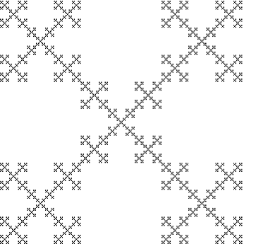
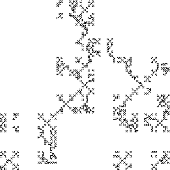
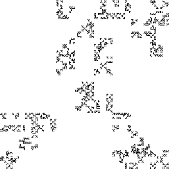
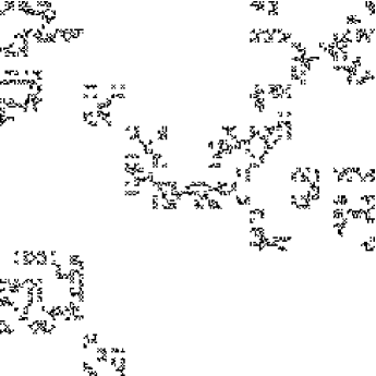
Figure 1: Randomly rearranged fractals of size $N=7$; $p=0$ (left) and $p=0.2$ (right)

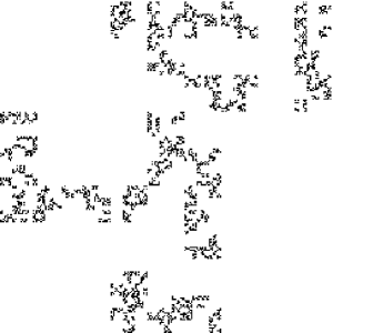
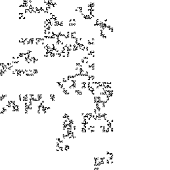
Figure 2: Randomly rearranged fractals of size $N=7$; $p=0.4$ (left) and $p=0.6$ (right)

Figure 3: Randomly rearranged fractals of size $N=7$; $p=0.8$ (left) and $p=1$ (right)

2.3 Measurement of Hierarchical Modularity

In Ref. [11] several methods for measuring the dimension of regular fractals were compared. In order to quantify modularity, we apply the box counting method, where we cover growing regions of the fractal with a growing square window started from the centre, and at each step we count the mass (the number of elementary blocks) inside the window. By this means, one gets a mass function: the inside mass of the fractal as a function of the linear size of the window. As pointed out in Ref. [11], for regular fractals this mass function is not a straight line in a log-log plot: There are periodic deviations due to the above mentioned separation of scales, i.e., due to modularity. Therefore we consider the periodicity of these deviations from the straight lines as the measure of modularity.
From our model, presented in Sec. 2.2, one gets different deviation functions for different values of $p$. In order to analyse these functions we applied Fast Fourier Transform (FFT) to them.

2.4 Results

In this subsection we discuss the results of the measurement of modularity described above in Sec. 2.3.

The log-log plots of the mass deviation functions as a function of the window size are plotted in Fig. 4 for different values of parameter $p$. For non-zero $p$, each curve is the average of $200$ randomly rearranged fractals (with same $p$).

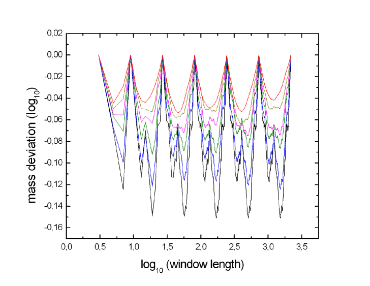
Figure 4: The deviation functions for fractals $N=7$ at different levels of randomization. The value of $p$ decreases by $0.2$ from above ($p=1$, red) to below ($p=0$, black). In cases $p\neq 0$ we averaged 200 randomly rearranged fractals.

Apparently, the mass deviation functions reflect the hierarchical modularity of the fractals of different $p$ values. In the $p=0$ case, the function has an inherent structure corresponding to its high degree of modularity. This scale-free structure is more visible on the farther periods of the function, because there we have more points. This inherent structure of the curves vanishes as $p\rightarrow 1$. The maximum deviation also decreases as we increase $p$, and the functions become smoother and smoother (apart from the basic high peaks with values of $0$), indicating the vanishing modularity of the fractals. The $0$-valued peaks correspond to powers of $3$: when the linear size of the window reaches powers of $3$, the window contains a whole sub-fractal with the exact dimension. This is the consequence of not mixing the elements in a continuous way. The deviation is non-positive for all values of $p$, which can be explained by the geometry of the applied rectangular windowing method in our special case.
The vanishing modularity could be better represented taking the FFT spectrum of the functions in Fig. 4. We analysed the last three periods of the functions with FFT, where they have the finest inherent structure. The results are plotted in Fig. 5.

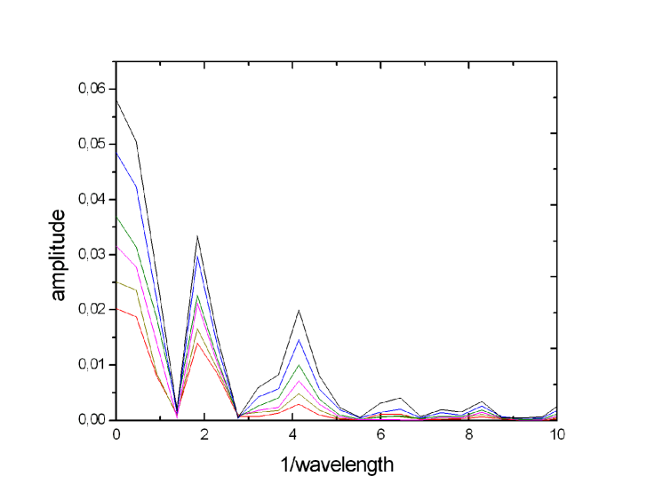
Figure 5: The FFT spectrum of the deviation functions of Fig. 4. The value of $p$ increases by $0.2$ from above ($p=0$, black) to below ($p=1$, red).

Because of the triadic organization of the fractals, the fundamental spatial frequency is $f=1/\log 3\approx 2.096$. This corresponds to the $0$-valued peaks mentioned above, therefore the first peaks in the FFT spectra are direct consequences of the geometry of our method. For the regular fractal ($p=0$) one could notice the first, second and third harmonics which indicate the scale-free property of the deviation function. The first harmonics, which indicates the fine structure of the deviation functions, significantly decreases for increasing values of $p$, and the second and third harmonics totally disappear, what verifies the decreasing degree of hierarchical modularity of the fractals for increasing rearrangement probability $p$.

3 MODULARITY OF NETWORKS

3.1 The Randomization of the Hierarchical Network Model

Our starting point was the deterministic, modular hierarchical network model of Ravasz and Barabási [3] (see Fig. 6).

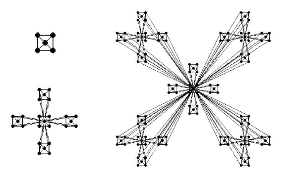
Figure 6: The deterministic hierarchical network at different sizes [3]

Its main features correspond to the real networks [3]: the degree distribution is scale-free, the clustering coefficient is independent of the size, and follows a power-law as a function of degree: $C(k)\propto k^{-\alpha}$. In real networks, $\alpha$ is usually about 1.
The regular model also has obviously hierarchically modular structure. As real grown networks are to some extent random, the question raises how the modularity is influenced by the randomness. In order study this problem, we used a link randomization procedure, earlier already applied to investigate the influence of randomness on synchronization [12]. In this model two links were chosen randomly, and one node of both links was exchanged between the two links. This process was executed $M\times p$ times, where $M$ is the number of the links and $p$ is the control parameter of the randomization. This method conserves the degree distribution, as it does not change the degree of any node.
As $p$ increases from $0$ to $1$, the average clustering coefficient $\bar{C}$ first falls rapidly then becomes constant (see Fig. 7).

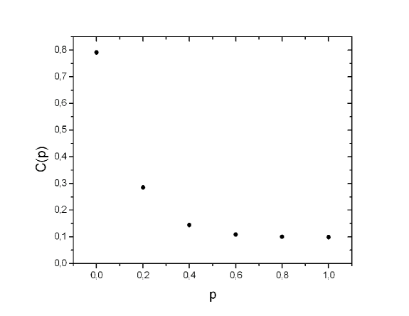
Figure 7: The clustering coefficient as a function of the randomization. Each point represents $200$ networks of $3125$ nodes.

For $p=1$, the degree dependence of $C(k)$ has two regions. It seems that the very low degree ($k<10$) nodes’ behavior is significantly different from the rest. Due to this effect and to the crossover it causes, the asymptotics sets in rather late. However, it is clear that the distribution is very broad and it has possibly a power law tail (Fig. 8). Also due to the small $k$ anomaly the average $C$ decrease with increasing system size for the considered number of nodes.

Figure 8: Clustering as a function of degree. The slope of the dotted line is $-0.913$. From the average of $400$ networks of $78125$ nodes, $p=1$.

3.2 Topological Overlap Matrix

To investigate the presence or absence of modules and hierarchical structure, we used the topological overlap matrix (TOM) of the network [5]. The $ij$ element of this matrix, $T_{ij}$ equals the number of mutual neighbours of the nodes $i$ and $j$ (plus $1$ if $i$ and $j$ are connected), normalized by the minimum degree of $i$ and $j$, so $T_{ij}$ is between $0$ and $1$. Thus, the $i$-th row and column represents the overlap of the node $i$ with the other nodes of the network ($T_{ii}$ is defined as $1$). If there is an isolated module of densely interconnected nodes in the network, and rows/columns representing the nodes of the module are close to each other in the topological overlap matrix, the module appears in the matrix as a square centred on the diagonal with elements close to $1$. Of course, to enable this interpretation, the right sequence of the nodes has to be determined, just according to their overlap values, as it is outlined in the next paragraph. The hierarchy of modules is represented by a system of smaller and smaller (and more and more cohesive) squares embedded into the larger squares (in which the overlap of the modules decreases with the module size). These features can be easily observed on the matrix of the deterministic model (Fig. 9).

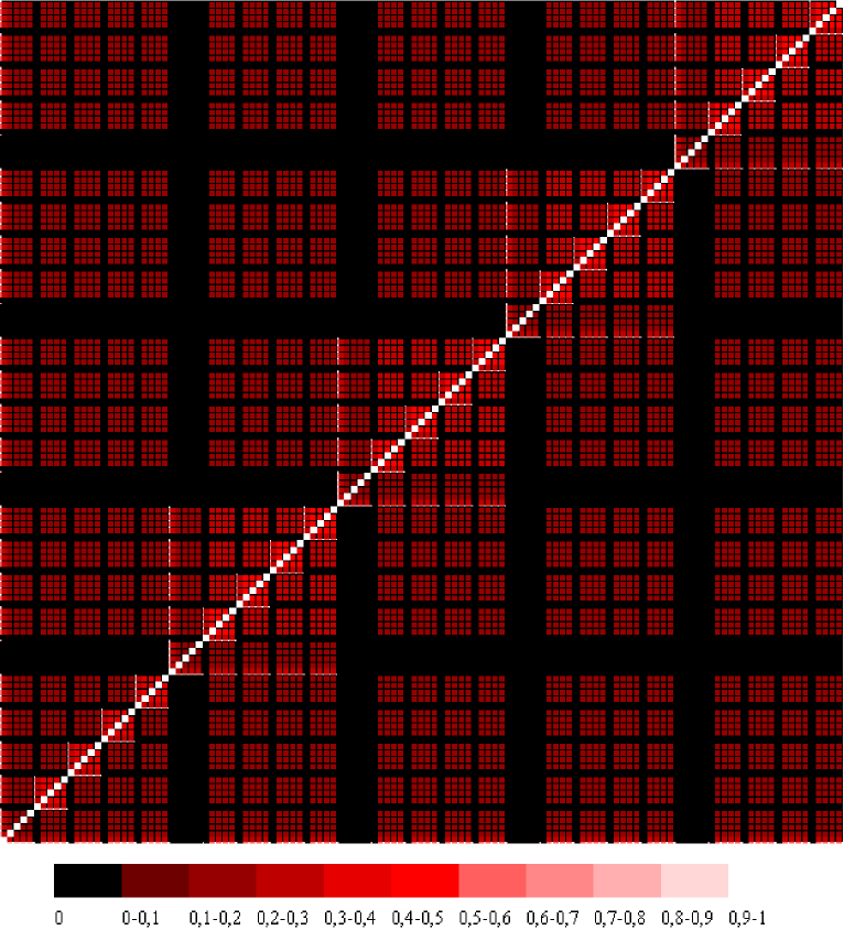
Figure 9: Topological overlap matrix of the original deterministic hierarchical network. The number of nodes is $625$.

The sequence of the rows/columns representing the nodes in the matrix is essential to recognize the modules and hierarchy. The rows/columns concerning nodes with big overlap have to be next to each other in the TOM, forming squares centred on the diagonal. In order to get the right sequence, we slightly modified the average linkage clustering method [5, 8]. The original algorithm builds communities joining nodes into ’supernodes’ (see Fig. ??: hierarchical tree, after a contraction the order in the new supernode has to be determined). In each step two nodes are joined, meanwhile the TOM decreases by one row and column.
The basic steps of the algorithm:

• First it finds the highest element in the TOM and contracts the two corresponding nodes into a supernode.

• The corresponding rows and columns of the two original nodes in the matrix are contracted into 1 row and 1 column (matrix elements are averaged), then the next round is started.

• This procedure is repeated until the TOM decreases into a $1\times 1$ matrix (every node joined into one supernode).

The previous steps describe the original algorithm. Because it was unable to reconstruct even the simple regular case shown on Fig. 9, some modifications were applied:

• It is possible that the above algorithm finds more than one elements with the same high value in the same step. In this case the contraction resulting the smallest supernode is performed. If this quantity is also degenerated, then the choice is made at random. The goal of this modification is to make the growing of the supernodes

• We are searching for clusters, not just pairs. Therefore the algorithm examines that the selected contraction is good from the view of building a cluster (containing more than $2$ nodes). If a better contraction is possible, that will be executed.

This way a sequence of contractions emerges. Parallel with the above algorithm placing the contracted nodes next to each other, the ’clustered’ sequence of the nodes appear. To make the above algorithm more clear, there is a small example:

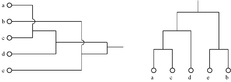
Figure 10: On the left-hand side, the contraction process is shown for $6$ nodes. On the right-hand side, the resulting dendogram is displayed. Below: the corresponding matrices at timestep $t=0\textrm{(the original TOM)},1,2,3$. The grey characters are out of interest.

0 a b c d e a $.1$ $.7$ $.5$ $.3$ b $.2$ $.1$ $.3$ c $.4$ $.3$ d $.3$ a

1 ac b e d e ac $.15$ $.3$ $.45$ $.3$ b $.3$ $.1$ $.3$ e $.3$ $.3$ d $.3$ a

2 acd b e d e acd $.13$ $.3$ $.45$ $.3$ b $.3$ $.1$ $.3$ e $.3$ $.3$ d $.3$

3 acd be e d e acd $.215$ $.3$ $.45$ $.3$ b $.3$ $.1$ $.3$ e $.3$ $.3$ d $.3$

Applying this algorithm, the TOM of the randomized deterministic network is visually interpretable (Fig. 11):

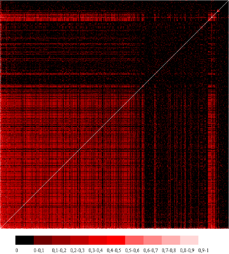
Figure 11: The topological overlap matrix of the randomized ($p=1$) deterministic hierarchical network ($625$ nodes).

modular organization is not recognizable with this clustering algorithm after the randomization process for $p=1$. This network is therefore scale free, it has a broad, probably power law $C(k)$ distribution – without a modular structure.
We would like to make the vanishing of the regular modularity quantitatively accessible in a similar way as in the case of the fractals: First, the elements of the TOM are raised to the third power in order to weaken the influence of the many small elements (to ´make contrast´). Then the elements are projected (summed) perpendicular to the diagonal (note that it means $2N-1$ sums for a $N\times N$ matrix), and the result is Fourier-analysed (Fig. 12).

Figure 12: FFT spectra of topological overlap matrices. Each curve represents an averaged spectrum over 500 networks of 625 nodes for $p=0$ (a), $0.01$ (b), $0.05$ (c), $0.2$ (d), $0.4$ (e), $1$ (f).

A peak in the average of the amplitude-spectra indicates the presence of equal-sized modules. As $p$ increases from zero, the peaks indicating the presence of the 5-node and 25-node modules are decreasing to zero rapidly (see Fig. 13).

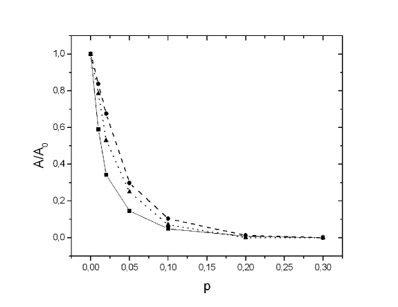
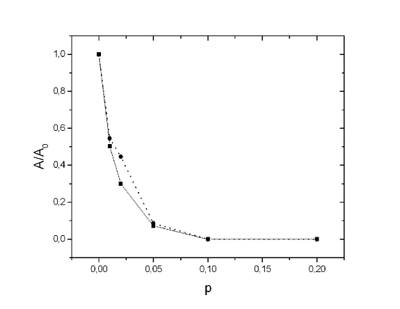
Figure 13: FFT peaks corresponding to the $5$- (a) and $25$-node (b) clusters of the deterministic, hierarchical network as functions of randomization, averages over $500$ networks of size $625$ (squares), $125$ (circles), $25$ (triangles). The amplitudes are normalized by the value corresponding to $p=0$.

4 DISCUSSION

In this paper we analysed the effect of randomness on the hierarchical modularity of scale free structures. The quantitative analysis was based on an important feature of modularity: the separation of scales. We studied regular structures (Vicsek snowflake, deterministic modular network) where randomness was introduced such that scale freeness and other features (broad distribution of $C(k)$) were maintained. Appropriate characteristics of modularity were chosen using Fourier components of the mass deviation function (for fractals) or of projections of the elements of the TOM (networks). In both cases we observed a significant decrease of hierarchical modularity with increasing randomness. For networks, we also observed a rapid fall for small values of $p$ in the clustering coefficient and in the Fourier peaks, suggesting a crossover similar to the phenomenon described in Ref. [12].

It has to be emphasized that the applicability of the Fourier analysis is based on the fact that the regular, hierarchical structures had a regular scale separation. If the separation of scales is less regular, hierarchical modularity can still exist, however, sufficient randomization would destroy it in this case too. In many real networks signatures of hierarchical modularity could be found [3] and the same is true for some model networks like the Holme-Kim [13, 14] network [15]. This indicates that the level of irregularity in these networks is far from that reached by randomization in our models.

5 ACKNOWLEDGEMENTS

Thanks are due to T. Vicsek, E. Ravasz and A.-L. Barabási for important discussions.

References

- [1] R. Albert, A-L. Barabási: Statistical Mechanics of Complex Networks, Rev. Mod. Phys. 74, pp. 47-97 (2002)
- [2] M.E.J. Newman: The structure and function of complex networks, SIAM Review 45, pp. 167-256 (2003)
- [3] E. Ravasz, A-L. Barabási: Hierarchical organization in complex networks, Phys. Rev. E 67, 026112 (2003)
- [4] A-L. Barabási, Z. Dezsõ, E. Ravasz, S-H. Yook and Z. Oltvai: Scale-free and hierarchical structures in complex networks, Sitges Proceedings on Complex Networks (2002)
- [5] E. Ravasz, et al.: Hierarhical Organization of Modularity in Metabolic Networks, Science 297, pp. 1551-1555 (2002)
- [6] Z.N. Oltvai, A-L. Barabási: Life’s Complexity Pyramid, Science 298, pp. 763-764 (2002)
-
[7]
A. Clauset, M.E.J. Newman, and C. Moore: Finding
community structure in very large networks,
Phys. Rev. E 70, 066111 (2004),
G. Palla, I. Derényi, I. Farkas, and T. Vicsek, on community identification by clique percolation (to appear in Nature) - [8] M.B. Eisen, P.T. Spellman, P.O. Brown and D. Botstein: Cluster analysis and display of genome-wide expression patterns, Proc. Natl. Acad. Sci. USA 95, pp. 14863-14868 (1998)
- [9] S.M. Dorogovtsev, J. F. F. Mendes: Evolution of networks, Adv. Phys. 51, pp. 1079-1187 (2002)
- [10] T. Vicsek: Fractal Models for Diffusion Controlled Aggregation, J. Phys. A16, L647-651 (1983)
- [11] T. Tél, Á. Fülöp, T. Vicsek: Determination of fractal dimensions for geometrical multifractals, Physica A 159, pp. 155-166 (1989)
- [12] E. Oh, K. Rho, H. Hong, B. Kahng: Modular Synchronization in Complex Networks; arXiv:cond-mat/0408202 (2004)
- [13] P. Holme B.J. Kim, Phys. Rev. E 65, 026107 (2002)
- [14] G. Szabó, M. Alava, J. Kertész: Structural Transitions in Scale-free Networks; Phys. Rev. E 67, 056102 (2003)
- [15] E. Ravasz, private communication