Microcanonical Ensemble Extensive Thermodynamics of Tsallis Statistics

Abstract

The microscopic foundation of the generalized equilibrium statistical mechanics based on the Tsallis entropy is given by using the Gibbs idea of statistical ensembles of the classical and quantum mechanics. The equilibrium distribution functions are derived by the thermodynamic method based upon the use of the fundamental equation of thermodynamics and the statistical definition of the functions of the state of the system. It is shown that if the entropic index $\xi=1/(q-1)$ in the microcanonical ensemble is an extensive variable of the state of the system, then in the thermodynamic limit $\tilde{z}=1/(q-1)N=\mathrm{const}$ the principle of additivity and the zero law of thermodynamics are satisfied. In particular, the Tsallis entropy of the system is extensive and the temperature is intensive. Thus, the Tsallis statistics completely satisfies all the postulates of the equilibrium thermodynamics. Moreover, evaluation of the thermodynamic identities in the microcanonical ensemble is provided by the Euler theorem. The principle of additivity and the Euler theorem are explicitly proved by using the illustration of the classical microcanonical ideal gas in the thermodynamic limit.

I Introduction

The equilibrium statistical mechanics and thermodynamics are well defined theories in modern physics Gibbs ; Balescu . Applications of these theories are restricted by investigation of the so-called thermodynamic or statistical systems which are constrained by several rigid requirements Kvasn . One of the first attempts to construct the generalized equilibrium statistical mechanics based on the mathematical redefinition of the Boltzmann-Gibbs statistical entropy and the principles of the information theory belongs to C. Tsallis Tsal88 . Until recently, there has been a great deal of interest in studying nonextensive thermodynamics due to its relevance in many fields of physics Tsal99 ; Gudima . However, many fundamental features regarding the violation of the zero law of thermodynamics and the principle of additivity remain unclear Abe0 ; Parv1 . Note that these difficulties have resulted in the occurrence of a large number of variants of the Tsallis generalized statistical mechanics Tsal98 .

The statistical mechanics investigates thermodynamic systems which are defined solely by the specification of macroscopic variables on the basis of the theory of probability and the microscopic laws of the classical and quantum mechanics. The evolution of the macroscopic system with a large number of degrees of freedom is impossible to describe by only dynamic methods. Therefore, the Gibbs idea of statistical ensembles is usually used Zub . All information about the macrostate of the system is contained in the phase distribution function, which evolves according to the Liouville equation or in the statistical operator whose evolution with time is described by the von Neumann equation. To derive the phase distribution function and the statistical operator is the primary goal of the nonequilibrium statistical mechanics.

In particular, the equilibrium statistical mechanics implies that one uses the Gibbs equilibrium statistical ensembles. In the state of thermodynamic equilibrium of the system, the phase distribution function and the statistical operator do not depend on time. Therefore, they are functions only of the first integrals of motion of the dynamic system. In this case, the mechanical laws and the Liouville and von Neumann equations do not allow one to determine unequivocally the equilibrium distribution function and the statistical operator Balescu ; Zub . Therefore, an obvious dependence of the equilibrium distributions on the macroscopic variables of the state of the system is defined by introducing additional postulates. The traditional way is based on the Gibbs postulate of the equiprobability of the dynamic states of the isolated system Gibbs . The alternative way rests on the Jaynes principle of a maximum of the information entropy Jaynes . The statistical mechanics constructed on the Gibbs equilibrium distributions, which corresponds to the Boltzmann-Gibbs statistical entropy, completely satisfies all postulates of the equilibrium thermodynamics.

Standard treatments of the Tsallis statistics point out that the entropic index $q$ is an additional intensive parameter, which has a fixed value for different thermodynamic systems Tsal98 . This concept leads to shortcomings of thermodynamics and needs to be reconsidered. As shown further, these problems can be resolved by the assumption that the parameter $\xi=1/(q-1)$ is the extensive argument of the statistical entropy.

The paper is organized as follows. In the second section, the microscopic foundation of the Tsallis generalized statistical mechanics is given. The microcanonical equilibrium distribution function and statistical operator are deduced in the third section. In the fourth section, the performance of the thermodynamic principles in the microcanonical ensemble of the Tsallis statistics are proved. The developed formalism is exemplified in the fifth section by treating the classical microcanonical ideal gas.

II Microscopic Foundation of Tsallis Statistical Mechanics

A macrostate of a system with a large number of degrees of freedom is imperfectly known at the microscopic level. The system can be found in any dynamic state compatible with the external macroscopic conditions. Therefore, for the macroscopic system it is possible to maintain only the probabilistic description of dynamic processes. For this reason, in the statistical mechanics the Gibbs idea of statistical ensembles is straightforward. The macroscopic state of the system is represented as a set of a large number of copies of the dynamic system under identical macroscopic conditions. Each system of the ensemble is represented by a point in phase space. Any physical observable $A$ of the macroscopic system is represented as the expectation value $\langle A\rangle^{t}$ of the dynamic variable $A(x,p,t)$ with the phase distribution function $\varrho(x,p,t)$. The evolution with time of a phase distribution function is governed by the Liouville equation. According to the Liouville theorem, the volume of a region in phase space remains constant in the process of movement of phase points. The phase distribution function is constant along the phase trajectories, $\varrho(x,p,t)=\varrho(x^{\prime},p^{\prime},t^{\prime})$. To describe the quantum many-particle systems the mixed states are considered. A macrostate thus appears as a set of possible microstates, which are set up by state vectors $|\Psi_{r}(t)\rangle$, $r=1,2,\ldots$, each with its own probability $w_{r}$ for its occurrence. The statistical operator $\varrho(t)$ allows to determine the expectation value of a dynamic variable $A$ regardless of the choice of the set of quantum states $\{|\Psi_{r}(t)\rangle\}$. The evolution with time of a statistical operator is governed by the von Neumann equation. In the state of thermal equilibrium of the macroscopic system, the phase distribution function $\varrho_{eq}(x,p)$ and the statistical operator $\varrho_{eq}$ should not depend on the time $t$. Therefore, from the Liouville and von Neumann equations it follows that they are the first integrals of motion which must depend only on the first constants of motion of the system. Moreover, if these quantities are unequivocal and additive, then there exist only four such integrals of motion: energy $H$, the total momentum vector $\mathbf{P}$, the total angular momentum vector $\mathbf{M}$, and the number of particles $N$. In Balescu ; Zub , the basic definition of the microscopic foundation of the statistical mechanics is explained in detail. The present investigation rests on this assumption.

The equilibrium distribution function and the equilibrium statistical operator are not determined unequivocally by the mechanical laws. To express the equilibrium distributions from the macroscopic variables of state, the introduction of additional postulates is required. A traditional way to construct the equilibrium distributions is based on the Gibbs postulate of the equiprobability of all accessible dynamic states of the isolated system Gibbs . An alternative way for this is based on the statistical definition of the entropy and the use of the Jaynes principle explored in the information theory Jaynes . In the present study, we suggest a new method based on the laws of the equilibrium thermodynamics.

For this reason, we briefly recall the general laws of the macroscopic equilibrium thermodynamics. The thermodynamic systems are the object of the equilibrium thermodynamics and they must satisfy some obligatory conditions Kvasn . First, these are the systems of a large number of particles interacting with each other and with external fields. Second, for every thermodynamic system the zero law of thermodynamics is fulfilled, i.e., for such a system there exists a state of thermal equilibrium, which eventually is reached by the system at the fixed external conditions. This principle guaranties the existence of the special thermal measure, the temperature $T$, which is a general characteristic of all thermodynamic systems in equilibrium contact and which does not depend on the place and the method of measurements.

Third, for thermodynamic systems the principle of additivity is valid: all variables belong to two classes of additivity, according to the reaction of a given physical one to the division of the equilibrium system into the equilibrium macroscopic parts, for example, into two parts. The extensive variables can be split into two parts, and they should be proportional to the actual amount of matter present, $\mathcal{F}_{1+2}=\mathcal{F}_{1}+\mathcal{F}_{2}$. On the other hand, the intensive variables have to keep its values and cannot depend on the size of the system, $\phi_{1+2}=\phi_{1}=\phi_{2}$. As an example, we may consider the thermodynamic systems which may be fixed in terms of the macroscopic variables of state $T,V,N$. In this case, the thermodynamic principle of additivity is implemented if intensive quantities are functions of intensive arguments, and extensive variables are proportional to the number of particles of the system multiplied by the intensive quantity. Such dependence of extensive and intensive variables is provided by the thermodynamic limit Kvasn . In this respect, all expressions have to be exposed to a formal limiting procedure $N\rightarrow\infty,V\rightarrow\infty,v=V/N=\mathrm{const}$, and only main asymptotics on $N$ should be kept. Then the extensive variables $\mathcal{F}$ can be written $(\alpha>0)$

$$\mathcal{F}(T,V,N)\left|{}_{N\rightarrow\infty\atop v=\mathrm{const}}\right.=N(f(T,v)+O(N^{-\alpha}))\stackrel{{\scriptstyle as}}{{=}}Nf(T,v),$$ (1)

whereas the intensive variables $\phi$ take the following form:

$$\phi(T,V,N)\left|{}_{N\rightarrow\infty\atop v=\mathrm{const}}\right.=\phi(T,v)+O(N^{-\alpha})\stackrel{{\scriptstyle as}}{{=}}\phi(T,v),$$ (2)

where $v=V/N$ is the specific volume and $f=\mathcal{F}/N$ is the specific $\mathcal{F}$. Note that the thermodynamic limit is a one-limiting procedure. The transitions not coordinated among themselves $N\rightarrow\infty$ and $V\rightarrow\infty$ have no physical sense, as in this case we would get results for either the superdense system or the empty one.

Fourth, in relation to the thermodynamic systems the first, the second and the third principles of thermodynamics are fulfilled, being the mathematical basis of the macroscopic theory. The first principle postulates the energy $E$ conservation law. The second principle of thermodynamics in the axiomatic formulation of R.J. Clausius postulates the existence of a function of state $S_{\mathrm{T}}$, called entropy. The absolute value of entropy is determined from the third law of thermodynamics or the Nernst theorem. The first and the second principles of thermodynamics for the quasistatic reversible processes are combined to give the fundamental equation of thermodynamics:

$$TdS_{\mathrm{T}}=dE+pdV+Xdz-\mu dN,$$ (3)

where $z=(z_{1},\ldots,z_{k})$ and $V$ are the ”thermodynamic coordinates”; $X=(X_{1},\ldots,X_{k})$ and $p$ play the role of the associated ”forces”; $\mu=\{\mu_{i}\}$ are the chemical potentials and $N=\{N_{i}\}$ are the number of particles for each kind $i$, respectively. The second law of thermodynamics for nonequilibrium states, also formulated by R.J. Clausius, refers to the irreversible processes. This principle gives the direction of a real process allowing one to investigate the properties of equilibrium states as extreme ones. The most complete account of the equilibrium and non-equilibrium processes and the role of the characteristic times in the macroscopic thermodynamics is found in Kvasn ; Prigogine .

The expectation values of a dynamic variables with the equilibrium distribution function and the equilibrium statistical operator must satisfy all the postulates of the equilibrium thermodynamics. The connection between the distribution function and the macroscopic thermodynamical variables of the state is provided by the statistical entropy. Usually it is determined on the base of the information entropy. Let us define the Tsallis information entropy, which recently has received wide popularity due to the property of nonextensivity and which is used for construction of the so-called generalized statistical mechanics Tsal88 ; Tsal98 . The Tsallis information entropy for the discrete distribution of probabilities $\{p_{i}\}$ for $W$ independent elementary events is defined in the following manner Tsal88 :

$$S_{\mathrm{inf}}=-k\sum\limits_{i=1}^{W}\frac{p_{i}-p_{i}^{q}}{1-q},\;\;\;\;\;\;\;\;\;\;\;\;\;\;\;\sum\limits_{i=1}^{W}p_{i}=1,$$ (4)

where $k$ is the Boltzmann constant and $q\in\mathbf{R}$ is the real parameter accepting values $0<q<\infty$. In the limit $q\to 1$, we come to the well-known expression for the Boltzmann-Gibbs-Shannon entropy, $S_{\mathrm{inf}}^{(BGS)}=-k\sum_{i=1}^{W}p_{i}\ln p_{i}$. The information entropy (4) is known as Havrda-Charvat-Daróczy-Tsallis entropy (see Rag99 ). However, in this paper, we shall use the short name for it. The information entropy is considered to be a measure of uncertainty of information concerning the statistical distribution $\{p_{i}\}$. The main its properties can be found in Tsal99 .

Let us introduce for further convenience a new representation for the Tsallis information entropy with a new parameter $\xi$

$$S_{\mathrm{inf}}=k\xi\sum\limits_{i=1}^{W}p_{i}(1-p_{i}^{1/\xi}),\;\;\;\;\;\;\;\;\;\;\;\;\xi=\frac{1}{q-1},$$ (5)

The parameter $\xi$ takes the values $-\infty\leq\xi\leq-1$ for $0<q\leq 1$ and $0<\xi\leq\infty$ for $1\leq q<\infty$. In particular, in the limiting case for the value of the parameter $q=1$, we have $\xi=\pm\infty$.

Now, the Tsallis statistical entropy in the classical and quantum mechanics can be defined as follows

$$S(t)=k\xi\int\varrho(x,p,t)[1-\varrho^{1/\xi}(x,p,t)]d\Gamma,\;\;\;\;\;\;\;\;\;\;\;S(t)=k\xi\mathrm{Tr}\{\varrho(t)[1-\varrho^{1/\xi}(t)]\},$$ (6)

where $\varrho(x,p,t)$ is the phase distribution function and $\varrho(t)$ is the statistical operator. It is easy to show that the Tsallis statistical entropy is not additive for the fixed value of $\xi$ and it is constant along the phase trajectories of the dynamic system. As the total time derivative from the phase distribution function is equal to zero, $d\varrho/dt=0$, valid from the Liouville equation and the Liouville theorem, the total time derivative from the classical entropy immediately yields the equality

$$\frac{dS(t)}{dt}=k\xi\int\frac{d\varrho(x,p,t)}{dt}[1-(1+\frac{1}{\xi})\varrho^{1/\xi}(x,p,t)]d\Gamma=0.$$ (7)

For the quantum ensembles, the Tsallis statistical entropy does not depend on time. Note that for the Gibbs statistical entropy this problem is inherent as well Zub .

III Microcanonical Ensemble

In this section, the microcanonical distribution function and the statistical operator will be expressed through the variables of state of the isolated system $(E,V,z,N)$. Let us consider the equilibrium statistical ensemble of the closed energetically isolated systems of $N$ particles at the constant volume $V$ and the thermodynamic coordinate $z$. It is supposed that all systems have identical energy $E$ within $\Delta E\ll E$.

To begin with, we turn to instances of the classical case. The Tsallis equilibrium statistical entropy (6) represents a function of the parameter $\xi$ and a functional of the equilibrium phase distribution function $\varrho_{eq}(x,p)$:

$$S(\xi,\{\varrho_{eq}\})=k\xi\int\limits_{D}\varrho_{eq}(x,p)(1-\varrho_{eq}^{1/\xi}(x,p))d\Gamma_{N},$$ (8)

where $d\Gamma_{N}=dxdp$ is an infinitesimal element of phase space. Let the phase distribution function $\varrho_{eq}(x,p)$ be distinct from zero only in the region of phase space $D$, which is defined by inequalities $E\leq H(x,p)\leq E+\Delta E$ and be normalized to unity:

$$\int\limits_{D}\varrho_{eq}(x,p)d\Gamma_{N}=1.$$ (9)

The phase distribution function depends on the first additive integrals of motion of the system. In particular, it is a function of the Hamiltonian, $\varrho_{eq}(x,p)=\varrho_{eq}(H(x,p))$. Moreover, the Hamilton function $H(x,p)$ has the parametrical dependence upon the number of particles $N$, volume $V$ of the system and $z$.

For an isolated system, in the state of thermal equilibrium the thermodynamic entropy $S_{\mathrm{T}}(E,V,z,N)$ has its maximal value. Hence, the fundamental equation of thermodynamics (3) for the quasiequilibrium processes is implemented. Changes of the variables of state at transition from one equilibrium state to another nearby state are equal to zero, $dE=0,dV=0,dz=0$ and $dN=0$. Therefore, from the basic equation of thermodynamics (3) it follows immediately that the thermodynamic entropy at the fixed values of $E,V,z,N$ is constant:

$$(dS_{\mathrm{T}})_{EVzN}=0.$$ (10)

To express the phase distribution function $\varrho_{eq}(x,p)$ through the variables of state $(E,V,z,N)$, let us replace the equilibrium thermodynamic entropy $S_{\mathrm{T}}$ of the macroscopic system with the Tsallis statistical one (8), $S_{\mathrm{T}}(E,V,z,N)\Longleftrightarrow S(\xi,\{\varrho_{eq}\})$, and substitute it in Eq. (10). Taking into account Eqs. (9) and (10), one finds

$$dS=\frac{\partial S}{\partial\xi}\ d\xi+\int\limits_{D}\frac{\delta S}{\delta\varrho_{eq}}\ d\varrho_{eq}\ d\Gamma_{N} = 0,$$ (11)

$$\int\limits_{D}d\varrho_{eq}\ d\Gamma_{N} = 0,$$ (12)

where the symbol $d$ before the functions $S,\xi$ and $\varrho_{eq}$ is the total differential in variables $(E,V,z,N)$. One should note that the unequivocal conformity between statistical and thermodynamic entropies is satisfied for the case where the parameters $\xi$ and $\{\varrho_{eq}\}$ are the functions of the variables of state $(E,V,z,N)$ of the isolated system. Let us put

$$\xi=\frac{1}{q-1}=z.$$ (13)

Since $d\xi=0$ and $d\varrho_{eq}=0$, we obtain from Eqs. (11) and (12),

$$\frac{\delta S(z,\{\varrho_{eq}\})}{\delta\varrho_{eq}}=k\alpha,$$ (14)

where $\alpha$ is a certain constant, and $k$ is the Boltzmann constant, which was introduced for convenience. Substituting Eq. (8) into (14), we obtain

$$\varrho_{eq}^{1/z}(x,p;E,V,z,N)=\frac{z-\alpha}{z+1}.$$ (15)

The parameter $\alpha$ has been eliminated by using Eqs. (8) and (9):

$$\varrho_{eq}(x,p;E,V,z,N)=\left[1-\frac{S}{kz}\right]^{z}.$$ (16)

Equations (16) and (9) together give

$$\left[1-\frac{S}{kz}\right]^{-z}=\int\limits_{D}d\Gamma_{N}=\int\Delta(H(x,p)-E)d\Gamma_{N}\equiv W(E,V,N),$$ (17)

where $\Delta(\varepsilon)$ is the function distinct from zero only in the interval $0\leq\varepsilon\leq\Delta E$, where it is equal to unit. The statistical weight $W(E,V,N)$ is meant as a dimensionless phase volume, i.e., the number of dynamic states inside a layer $\Delta E$. Based on this, we get the equipartition probability from Eq. (16) as a function of the thermodynamic ensemble variables, energy $E$, volume $V$, number of particle $N$, and parameter $z$ Zub :

$$\varrho_{eq}(x,p;E,V,z,N)=W^{-1}(E,V,N)\Delta(H(x,p)-E).$$ (18)

Thus, using Eq. (17), we can write the entropy as (cf. Tsal88 ; Gross )

$$S(E,V,z,N)=kz[1-W^{-1/z}(E,V,N)]=kz[1-e^{-S_{\mathrm{G}}(E,V,N)/kz}],$$ (19)

where $S_{\mathrm{G}}$ is the Gibbs entropy Gibbs ; Zub for the microcanonical ensemble $(E,V,N)$:

$$S_{\mathrm{G}}(E,V,N)=k\ln W(E,V,N).$$ (20)

The quantum microcanonical ensemble and the corresponding equilibrium distribution function are in some respects analogous to the familiar classical ones. Let the probability distribution for quantum states of the system be different from zero only in the layer $E\leq E_{i}\leq E+\Delta E$ and be normalized to unity:

$$\sum\limits_{i}w_{i}=1,\;\;\;\;\;\;\;\;\;E\leq E_{i}\leq E+\Delta E.$$ (21)

The Tsallis equilibrium statistical entropy is a function of the parameter $\xi$ and probabilities $\{w_{i}\}$:

$$S(\xi,\{w_{i}\})=k\xi\sum\limits_{i}w_{i}(1-w_{i}^{1/\xi}).$$ (22)

The repeated use of the above procedure will lead us to the formula

$$\left[1-\frac{S}{kz}\right]^{-z}=\sum\limits_{i}\Delta(E_{i}-E)\equiv W(E,V,N).$$ (23)

The statistical weight $W(E,V,N)$ is equal to the number of quantum states in the layer $\Delta E$. The quantum microcanonical distribution becomes

$$w_{i}(E,V,z,N)=W^{-1}(E,V,N)\Delta(E_{i}-E).$$ (24)

The statistical operator corresponding to the microcanonical distribution of probabilities of quantum states (24) can be written as Zub

$$\varrho_{eq}(E,V,z,N)=W^{-1}(E,V,N)\Delta(H-E),$$ (25)

where the operator function $\Delta(H-E)$ is determined in the diagonal representation by the matrix elements $\langle k|\Delta(H-E)|k^{\prime}\rangle=\Delta(E_{k}-E)\delta_{kk^{\prime}}$. The quantum statistical entropy is calculated similarly to the classical one (19) with statistical weight (23). Note that the classical and quantum microcanonical distributions (18) and (24) are extreme equilibrium ones which correspond to a maximum of the Tsallis statistical entropy Tsal88 . The distribution functions (18) and (24) obtained by the thermodynamic method described here are identical with ones obtained by the Jaynes principle. The index $q$ for the Jaynes principle is a fixed parameter and does not depend on the variables of state of the system. In this case, the Tsallis statistics does not satisfy the zero law of thermodynamics Parv1 .

IV Thermodynamics of microcanonical ensemble

It is well-known from the conventional statistical mechanics that in the thermal equilibrium the Gibbs entropy of the microcanonical ensemble is an extensive variable, and it has all peculiarities of the thermodynamic entropy in the thermodynamic limit Kvasn ; Zub . Mathematically, this implies that the Gibbs entropy $S_{\mathrm{G}}$ is a homogeneous function of variables $E,V$ and $N$ of the first order, i.e., one has the following property Prigogine :

$$S_{\mathrm{G}}(\lambda E,\lambda V,\lambda N)=\lambda S_{\mathrm{G}}(E,V,N),$$ (26)

where $\lambda$ is a certain constant. After substitution of Eq. (20) into (26), it is easy to check up that the statistical weight $W$ must satisfy the following requirement:

$$W(\lambda E,\lambda V,\lambda N)=W^{\lambda}(E,V,N).$$ (27)

Taking into account Eqs. (19) and (26), one finds the following peculiarity of the Tsallis entropy

$$S(\lambda E,\lambda V,\lambda z,\lambda N)=\lambda S(E,V,z,N),$$ (28)

which shows that the Tsallis entropy in the microcanonical ensemble is a homogeneous function of variables $E,V,z,N$ of the first order. In other words, it is extensive. It is essential to make clear that the homogeneity property of quantities (26)-(28) is realized only in the thermodynamic limit.

Differentiating Eq. (28) with respect to $\lambda$, and putting $\lambda=1$, we obtain the well-known Euler theorem for the homogeneous functions:

$$E\left(\frac{\partial S}{\partial E}\right)_{V,z,N}+V\left(\frac{\partial S}{\partial V}\right)_{E,z,N}+z\left(\frac{\partial S}{\partial z}\right)_{E,V,N}+N\left(\frac{\partial S}{\partial N}\right)_{E,V,z}=S.$$ (29)

Using the thermodynamic relations following from the fundamental equation of thermodynamics (3) in case of the isolated thermodynamic system $(E,V,z,N)$

$$\left(\frac{\partial S}{\partial E}\right)_{V,z,N}=\frac{1}{T},\;\;\;\left(\frac{\partial S}{\partial V}\right)_{E,z,N}=\frac{p}{T},\;\;\;\left(\frac{\partial S}{\partial z}\right)_{E,V,N}=\frac{X}{T},\;\;\;\;\left(\frac{\partial S}{\partial N}\right)_{E,V,z}=-\frac{\mu}{T},$$ (30)

we get the Euler theorem Prigogine :

$$TS=E+pV+Xz-\mu N.$$ (31)

Applying the differential operator with respect to the ensemble variables $(E,V,z,N)$ on Eq. (31), we obtain the fundamental equation of thermodynamics

$$TdS=dE+pdV+Xdz-\mu dN$$ (32)

and the Gibbs-Duhem relation Prigogine

$$SdT=Vdp+zdX-Nd\mu.$$ (33)

Equation (33) means that the variables $T$, $\mu$, $X$ and $p$ are not independent. The fundamental equation of thermodynamics (32) provides the first principle

$$\delta Q=dE+pdV+Xdz-\mu dN$$ (34)

and the second law of thermodynamics

$$dS=\frac{\delta Q}{T}.$$ (35)

Here $\delta Q$ is a heat transfer by the system to the environment for quasistatic transition of the system from one equilibrium state to another nearby state.

Let us investigate the homogeneity properties of the variables $T,p,\mu$ and $X$. Substituting Eq. (19) into (30), we obtain the following expressions for the temperature $T$ Parv1 :

$$T(E,V,z,N)=T_{\mathrm{G}}(E,V,N)\ W^{1/z}(E,V,N)=T_{\mathrm{G}}(E,V,N)\ e^{S_{\mathrm{G}}(E,V,N)/kz}$$ (36)

and the variable $X$

$$X(E,V,z,N)=kT_{\mathrm{G}}(E,V,N)[e^{S_{\mathrm{G}}(E,V,N)/kz}-1-S_{\mathrm{G}}(E,V,N)/kz].$$ (37)

The pressure and the chemical potential of the system are equivalent with the pressure $p_{\mathrm{G}}$ and the chemical potential $\mu_{\mathrm{G}}$ of the Gibbs statistics, respectively, $p(E,V,z,N)=p_{\mathrm{G}}(E,V,N)$ and $\mu(E,V,z,N)=\mu_{\mathrm{G}}(E,V,N)$. These equations were derived by using the thermodynamic relations for the temperature $T_{\mathrm{G}}$, the pressure $p_{\mathrm{G}}$ and the chemical potential $\mu_{\mathrm{G}}$ of the Gibbs statistics, and taking into account Eq. (20):

$$\frac{1}{T_{\mathrm{G}}}=\left(\frac{\partial S_{\mathrm{G}}}{\partial E}\right)_{V,N},\;\;\;\;\;\;\;\frac{p_{\mathrm{G}}}{T_{\mathrm{G}}}=\left(\frac{\partial S_{\mathrm{G}}}{\partial V}\right)_{E,N},\;\;\;\;\;\;\;-\frac{\mu_{\mathrm{G}}}{T_{\mathrm{G}}}=\left(\frac{\partial S_{\mathrm{G}}}{\partial N}\right)_{E,V}.$$ (38)

The Gibbs quantities $T_{\mathrm{G}},p_{\mathrm{G}},\mu_{\mathrm{G}}$ are the homogeneous functions of the variables of state $(E,V,N)$ of the zero order. This can be proved by using Eqs. (38) and (26). Then, a combination of Eqs. (36) and (26) allows us to write the relation for the temperature $T$:

$$T(\lambda E,\lambda V,\lambda z,\lambda N)=T(E,V,z,N).$$ (39)

Similarly to Eq. (39), the relations for the pressure $p(\lambda E,\lambda V,\lambda z,\lambda N)$, the chemical potential $\mu(\lambda E,\lambda V,\lambda z,\lambda N)$, and the variable $X(\lambda E,\lambda V,\lambda z,\lambda N)$ are fulfilled. Thus, the temperature $T$, the pressure $p$, the chemical potential $\mu$, and quantity $X$ are the homogeneous functions of the variables $E,V,z,N$ of the zero order. So they are intensive variables Prigogine .

Let us prove in more detail the thermodynamic principle of additivity Kvasn . For instance, we assume that $\lambda=1/N$ and introduce the following specific variables:

$$\varepsilon=\frac{E}{N},\;\;\;\;\;\;\;\;\;\;\;\;\;\;v=\frac{V}{N},\;\;\;\;\;\;\;\;\;\;\;\;\;\;\;\;\;\tilde{z}=\frac{z}{N}=\frac{1}{(q-1)N}.$$ (40)

Thus, Eqs. (28) and (39) for the entropy and the temperature of the system, by using (40) with respect to $\lambda=1/N$, can be rewritten as

$$s(\varepsilon,v,\tilde{z})=\frac{1}{N}\ S(E,V,z,N)$$ (41)

and

$$T(\varepsilon,v,\tilde{z})=T(E,V,z,N),$$ (42)

where $s(\varepsilon,v,\tilde{z})$ is the specific entropy, $s=S/N$, which depends only on the intensive variables $\varepsilon,v$ and $\tilde{z}$. For the pressure $p$, the chemical potential $\mu$, and $X$, we have equations similar to that for the temperature (42). So, comparing Eqs. (41) and (42) with the thermodynamic equations (1) and (2), we conclude that the entropy $S$ is an extensive variable, as it is proportional to the number of particles $N$ multiplied by an intensive variable $s$, but the temperature $T$, the pressure $p$, the chemical potential $\mu$, and $X$ are intensive variables.

Let us divide the system into two parts ($1$ and $2$) and require that the total number of particles of the system should be equal to the sum of the number of particles of each subsystem separately and the specific quantities (40) should be equal among themselves

$$N_{1+2}=N_{1}+N_{2},\;\;\;\;\;\;\;\varepsilon_{1+2}=\varepsilon_{1}=\varepsilon_{2},\;\;\;\;\;\;\;v_{1+2}=v_{1}=v_{2},\;\;\;\;\;\;\tilde{z}_{1+2}=\tilde{z}_{1}=\tilde{z}_{2}.$$ (43)

Then, the variables $E,V$ and $z$ are extensive. Taking into account Eq. (43), one finds

$$s_{1+2}(\varepsilon_{1+2},v_{1+2},\tilde{z}_{1+2})=s_{1}(\varepsilon_{1},v_{1},\tilde{z}_{1})=s_{2}(\varepsilon_{2},v_{2},\tilde{z}_{2}).$$ (44)

Multiplying it by the first equation from (43) and using (41), we get

$$S_{1+2}(E_{1+2},V_{1+2},z_{1+2},N_{1+2})=S_{1}(E_{1},V_{1},z_{1},N_{1})+S_{2}(E_{2},V_{2},z_{2},N_{2}).$$ (45)

Thus, in the microcanonical ensemble the Tsallis entropy is an extensive variable. Furthermore, Eqs. (42) and (43) allow us to write

$$T_{1+2}(E_{1+2},V_{1+2},z_{1+2},N_{1+2})=T_{1}(E_{1},V_{1},z_{1},N_{1})=T_{2}(E_{2},V_{2},z_{2},N_{2}).$$ (46)

So, in the thermodynamic limit, the zero law of thermodynamics and the thermodynamic principle of additivity (see. (1) and (2)) for the Tsallis statistics in the microcanonical ensemble are valid. Here, the thermodynamic limit denotes the limiting statistical procedure $N\rightarrow\infty$ at $\varepsilon=\mathrm{const},v=\mathrm{const}$, and $\tilde{z}=\mathrm{const}$ with keeping the main asymptotics on $N$. This may be explicitly seen by making an expansion of the functions of the state in powers of the small parameter $1/N$ ($N\gg 1$$,|z|\gg 1$, i.e. $q\neq 1$) with the large finite values of the variables $E,V,z$. For the extensive functions the term proportional to $N$ is held and for the intensive variables only the term proportional to $N^{0}$ is kept (cf. Eqs. (1) and (2)). Note that the correct thermodynamic limit, $(q-1)N=\mathrm{const}$, for the Tsallis statistics has already been discussed in Botet et al. Botet1 ; Botet . In Abe Abe1 , the thermodynamic limit for the Tsallis statistics is wrong because the limits $N\to\infty$ and $|z|\to\infty$ are not coordinated among themselves. This procedure destroys the connection between the variables $N$ and $z$ in the functions of the state of the system (see Section II). In the case of the Boltzmann-Gibbs limit we make an expansion of the functions of the state in powers of the small parameter $1/\tilde{z}$ ($|\tilde{z}|\gg 1$, $N\gg 1$, i.e. $q\to 1$) and hold only the zero term of the power expansion.

It is important to note that some authors Abe0 ; Vives to make the connection with the equilibrium thermodynamics interpret the equations similar to our Eqs. (19) and (36) as the extensive representation of the Tsallis statistics in the terms of the physical temperature. But, as was shown in Parv1 , these equations are only the transformation formulas from the Tsallis statistics to the new extensive one.

V The perfect gas

The thermodynamic principle of additivity can thoroughly be investigated in the framework of a classical nonrelativistic ideal gas. In the microcanonical ensemble $(E,V,z,N)$, the statistical weight (17) of the perfect gas of $N$ identical nucleons is given by Das

$$W(E,V,N)=\frac{V^{N}}{N!}\int\frac{d^{3}p_{1}\ldots d^{3}p_{N}}{(2\pi\hbar)^{3N}}\ \delta\left(\sum\limits_{i=1}^{N}\frac{\vec{p}_{i}^{2}}{2m}-E\right)=\frac{V^{N}}{N!}\left(\frac{m}{2\pi\hbar^{2}}\right)^{\frac{3}{2}N}\frac{E^{\frac{3}{2}N-1}}{\Gamma(\frac{3}{2}N)},$$ (47)

where $m$ is the nucleon mass. In the thermodynamic limit ($N\gg 1$, $\varepsilon=E/N=\mathrm{const}$, $v=V/N=\mathrm{const}$) from Eq. (47), it follows immediately that Kvasn

$$W^{1/N}(E,V,N)=v\left(\frac{m\varepsilon e^{5/3}}{3\pi\hbar^{2}}\right)^{3/2}\equiv w(\varepsilon,v).$$ (48)

So Eq. (48) proves relation (27) for the statistical weight $W$ with $\lambda=1/N$. Then, the Tsallis entropy (19) is reduced to

$$S(E,V,z,N)=Ns(\varepsilon,v,\tilde{z}),\;\;\;\;\;\;\;\;\;\;s(\varepsilon,v,\tilde{z})=k\tilde{z}\left[1-w^{-1/\tilde{z}}\right].$$ (49)

Comparing Eq. (49) with (1), we conclude that the Tsallis entropy is an extensive variable. Note that in the limit $\tilde{z}\rightarrow\pm\infty$, we obtain the formula for the Gibbs specific entropy:

$$\left.s(\varepsilon,v,\tilde{z})\right|_{\tilde{z}\rightarrow\pm\infty}=k\ln w\equiv s_{\mathrm{G}}(\varepsilon,v).$$ (50)

Substituting (49) into (30), we get

$$T(E,V,z,N)=\frac{2}{3}\frac{\varepsilon}{k}w^{1/\tilde{z}}\equiv T(\varepsilon,v,\tilde{z}).$$ (51)

The temperature (51) is a function of the specific variables $\varepsilon,v$ and $\tilde{z}$. Therefore, it is an intensive variable by virtue of Eq. (2). In the limit $\tilde{z}\rightarrow\pm\infty$, we obtain the well-known formula for the Gibbs statistics

$$\left.T(\varepsilon,v,\tilde{z})\right|_{\tilde{z}\rightarrow\pm\infty}=\frac{2}{3}\frac{\varepsilon}{k}=T_{\mathrm{G}}(\varepsilon,v).$$ (52)

In a similar way, the pressure $p$, the chemical potential $\mu$, and $X$ become

$$p(E,V,z,N) = \frac{2}{3}\frac{\varepsilon}{v}\equiv p(\varepsilon,v,\tilde{z}),$$ (53)

$$\mu(E,V,z,N) = \frac{2}{3}\varepsilon\left[\frac{5}{2}-\ln w\right]\equiv\mu(\varepsilon,v,\tilde{z}),$$ (54)

$$X(E,V,z,N) = -\frac{2}{3}\varepsilon\left[1+\frac{1}{\tilde{z}}\ln w-w^{1/\tilde{z}}\right]\equiv X(\varepsilon,v,\tilde{z}).$$ (55)

Note that the pressure $p$ and the chemical potential $\mu$ for the classical ideal gas in the microcanonical ensemble do not depend on the parameter $\tilde{z}$, and they are equal to respective quantities of the Gibbs statistics. Then, Eqs. (49), (51), and (53)-(55) yield the Euler theorem (31) in terms of the specific variables

$$Ts=\varepsilon+pv-\mu+X\tilde{z}.$$ (56)

In the limit $\tilde{z}\rightarrow\pm\infty$, the pressure $p$ and the chemical potential $\mu$ remain unchanged but the variable $X=0$. So, by the example of the classical ideal gas the principle of additivity for the Tsallis statistics is proved. The Euler theorem (31) or (56) shows that in the Tsallis statistics the quantities $z=1/(q-1)$ and $X$ should be the variable of the state and the associated ”force”, respectively.

At this point one important quantity must be noted, the heat capacity $C_{V}=1/(\partial T/\partial E)_{V,z,N}$. In the framework of the ideal gas of $N$ nucleons it can be written as

$$C_{V}=\frac{3}{2}kNw^{-1/\tilde{z}}\left(1+\frac{3}{2}\frac{1}{\tilde{z}}\right)^{-1}.$$ (57)

Figure 1 shows the specific heat (left) and the temperature (center) vs the parameter $\tilde{z}$. The calculations are done for the system of nucleons at the specific energy $\varepsilon=50$ MeV and the specific volume $v=3/\rho_{0}$, where $\rho_{0}=0.168$ fm^-3. It is of great interest that both the heat capacity and the temperature sharply change their shape in the region of small values of $\tilde{z}$ and considerably defer from their Gibbs limit, which in the figure is indicated by arrows. In the region of $-3/2<\tilde{z}<0$, the heat capacity is negative. It is remarkable that such a behaviour has really been caused by the decrease of the temperature with $\varepsilon$. This dependence can be seen even better in right panel of Fig. 1 which shows the temperature vs the specific energy of the system for different values of the parameter $\tilde{z}$. The negative heat capacity in the microcanonical ensemble is closely related to the phase transition of the first order where the entropy is a convex function Chomaz ; Gross1 . The Fig. 1 clearly shows that the variable $\tilde{z}$ is the order parameter and the system is physically unstable in the region $-3/2<\tilde{z}<0$ at the fixed values of the variables $(v,\tilde{z})$, where the entropy is a convex function of $\varepsilon$. For example, entropy $s\sim\varepsilon^{3/2}$ at $\tilde{z}=-1$. Note that this critical feature of the system is not related with negative values of the parameter $q$ Tsal98 as we take into account the condition $1+1/N\tilde{z}>0$ ($N\gg 1$). The crossing point of all curves $(\varepsilon_{0},v_{0})$ in right panel of Fig. 1 is the point where the Tsallis and Gibbs entropies vanish, $S=0$ and $S_{G}=0$ or $w(\varepsilon_{0},v_{0})=1$. Thus, the following values of the energy $\varepsilon>\varepsilon_{0}$ and the volume $v>v_{0}$ of the system have the physical sense. Note that the temperature $T$ do not depend on energy $\varepsilon$ at $\tilde{z}=-3/2$ and it is equal with temperature $T_{0}=T(\varepsilon_{0},v_{0})$.

It should be remarked here that the microcanonical ensemble of the Tsallis statistics in the thermodynamic limit is equivalent with the canonical one. If we introduce the variable $z$ in the formulas for the perfect gas in the canonical ensemble of Abe et al. Abe0 ; Abe2 , then in the thermodynamic limit we recover the above functions of the state of the microcanonical ensemble. For instance, in the thermodynamic limit, Eq. (51) can be obtained from the energy $U_{q}(T,V,N)$ given in Abe0 ; Abe2 .

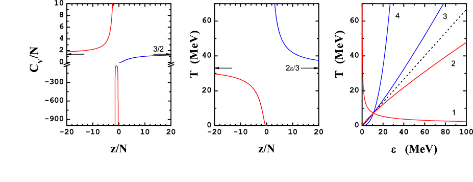
Figure 1: The dependence of the heat capacity (left) and the temperature (center) on the specific $\tilde{z}=z/N$ for the classical ideal gas of $N$ nucleons at the values of the specific energy $\varepsilon=50$ MeV and the specific volume $v=3/\rho_{0}$. The temperature as a function of the specific energy (right) for the different values of $\tilde{z}=-1$, $-10$, $10$ and $1$ (the curves $1,2,3$ and $4$, respectively) at $v=3/\rho_{0}$. The dashed line corresponds to the Gibbs statistics.

VI Conclusions

In this paper, we have explored the microscopic foundation of the generalized equilibrium statistical mechanics based on the Tsallis statistical entropy. The viewpoint utilized here considers that the microcanonical ensemble is most convenient to analyze the fundamental questions of the statistical mechanics. We summarize our main principles.

Here, the Gibbs idea of the statistical ensembles defined within the framework of the quantum and classical mechanics was used. In this approach, the equilibrium phase distribution function and the statistical operator do not depend on time, and they are functions of the additive first integrals of motion of the system by virtue of performance of Liouville and von Neumann equations. Additionally, these main quantities are functions of the macroscopic variables of state of the system. To derive the distribution functions, in contrast with the Jaynes principle, the new thermodynamic method based on the fundamental equation of thermodynamics and statistical definition of the functions of the state of the system was given.

In this paper, we have made the following claim. The index $\xi$ of the Tsallis entropy should be an extensive variable of the state of the system. As a result of this assumption, we obtain that in the microcanonical ensemble the Tsallis entropy represents the homogeneous function of the variables $E,V,z,N$ of the first order. The temperature of the system is an intensive variable, and, consequently, the zero law of thermodynamics is satisfied. Other functions of state of the system are either extensive or intensive. Thus, in the thermodynamic limit, $\tilde{z}=1/(q-1)N=\mathrm{const}$, in the Tsallis statistics the thermodynamic principle of additivity is carried out. Note that the Tsallis information entropy is nonextensive because the parameter $\xi$ is a certain intensive constant. Also it is necessary to note that the Tsallis statistical entropy as well as the Gibbs one has an essential lack. Both the entropies do not depend on time while the thermodynamic entropy grows up to achieve its maximal value in the state of thermal equilibrium. The extensive property of the Tsallis entropy in the microcanonical ensemble yields the Euler theorem which permits one to find the fundamental equation of thermodynamics and the Gibbs-Duhem relation. Thus, the first and the second principles of thermodynamics are fulfilled. Note that in the limit, $\tilde{z}\rightarrow\pm\infty$, all expressions of the Tsallis statistics take the form of the conventional Gibbs statistical mechanics. So the Tsallis statistical mechanics in the microcanonical ensemble satisfies all postulates of the equilibrium thermodynamics.

Finally, the classical nonrelativistic ideal gas of $N$ identical nucleons in the microcanonical ensemble was considered to illustrate the principles which were elucidated in the general theory. It has been shown that in the thermodynamic limit the statistical weight, the entropy, the temperature, and other quantities are the homogeneous functions of the first and zero order of the variables of state, respectively. Note that for ideal gas the Euler theorem was accomplished and in the limit, $\tilde{z}\rightarrow\pm\infty$, all expressions resembled ones of the Gibbs statistics.

Acknowledgments: This work has been supported by the Moldavian-US Bilateral Grants Program (CRDF project MP2-3045). We acknowledge valuable remarks and fruitful discussions with T.S. Biró, R. Botet, K.K. Gudima, M. Płoszajczak, and V.D. Toneev.

References

- (1) J.W. Gibbs, Elementary Principles in Statistical Mechanics, Developed with Especial Reference to the Rational Foundation of Thermodynamics, Yale Univ. Press, New Haven, 1902.
- (2) R. Balescu, Equilibrium and Nonequilibrium Statistical Mechanics, Wiley, New York, 1975.
- (3) I.A. Kvasnikov, Thermodynamics and Statistical Mechanics: The Equilibrium Theory [in russian], Moscow State Univ. Publ., Moscow, 1991.
- (4) C. Tsallis, J. Stat. Phys. 52 (1988) 479.
- (5) C. Tsallis, Braz. J. Phys. 29 (1999) 1, [arXiv:cond-mat/9903356].
- (6) K.K. Gudima, A.S. Parvan, M. Płoszajczak and V.D. Toneev, Phys. Rev. Lett. 85 (2000) 4691.
- (7) S. Abe, S. Martínez, F. Pennini, A. Plastino, Phys. Lett. A 281 (2001) 126.
- (8) A.S. Parvan and T.S. Biró, Phys. Lett. A 340 (2005) 375.
- (9) C. Tsallis, R.S. Mendes, A.R. Plastino, Physica A 261 (1998) 534.
- (10) D. Zubarev, V. Morozov and G. Röpke, Statistical Mechanics of Nonequilibrium Processes, Vol.1, Basic Concepts, Kinetic Theory, Akademie Verlag, Berlin, 1996.
- (11) E.T. Jaynes, Phys. Rev. 106 (1957) 620.
- (12) I. Prigogine, D. Kondepudi, Modern Thermodynamics: From Heat Engines to Dissipative Structures, John Wiley & Sons, Chichester, 1998.
- (13) G.A. Raggio, [arXiv:cond-mat/9909161].
- (14) D.H.E. Gross, Physica A 305 (2002) 99.
- (15) R. Botet, M. Płoszajczak and J.A. González, Phys. Rev. E 65 (2002) 015103(R).
- (16) R. Botet, M. Płoszajczak, K.K. Gudima, A.S. Parvan and V.D. Toneev, Physica A 344 (2004) 403.
-
(17)
S. Abe, Phys. Lett. A 263 (1999) 424;
S. Abe, Phys. Lett. A 267 (2000) 456, Erratum. - (18) E. Vives, A. Planes, Phys. Rev. Lett. 88 (2002) 020601.
- (19) C.B. Das and S.Das Gupta, Phys. Rev. C 64 (2001) 041601(R).
- (20) Ph. Chomaz, F. Gulminelli, Physica A 330 (2003) 451.
-
(21)
D.H.E. Gross, [arXiv:cond-mat/0508455];
D.H.E. Gross, Microcanonical thermodynamics: Phase transitions in ”Small” systems, volume 66 of Lecture Notes in Physics. World Scientific, Singapore, 2001. - (22) S. Abe, Physica A 269 (1999) 403.