Accurate polarization within a unified Wannier function formalism

Abstract

We present an alternative formalism for calculating the maximally localized Wannier functions in crystalline solids, obtaining an expression which is extremely simple and general. In particular, our scheme is exactly invariant under Brillouin zone folding, and therefore it extends trivially to the $\Gamma$-point case. We study the convergence properties of the Wannier functions, their quadratic spread and centers as obtained by our simplified technique. We show how this convergence can be drastically improved by a simple and inexpensive “refinement” step, which allows for very efficient and accurate calculations of the polarization in zero external field.

I Introduction

The representation of the one-particle electronic structure of molecules and solids in terms of localized Wannier wannier orbitals is nowadays “enjoying a revival” rmmartin as a useful tool for many applications mv ; hydrogen ; sharma ; cangiani ; fernandez ; posternak ; dovesi ; pavarini ; fabris ; feliciano ; danish . The main impetus for this renewal of interest was given by the establishment, by King-Smith and Vanderbilt (KSV), of a formally exact relationship between the sum of the Wannier function (WF) centers and a gauge-invariant Berry phase, in the context of the modern theory of polarization kingsmith . However, the intrinsic nonuniqueness in the Wannier function definition, and the difficulty in defining their centers within a periodic cell calculation, limited their practical use, until a particularly elegant method due to Marzari and Vanderbilt mv (MV) became available some years ago. Their scheme allows one to obtain, in a given isolated or extended system, a unique set of maximally localized Wannier functions that minimizes a well-defined spread functional. Moreover, the MV formalism provides as an important byproduct the positions of the WF centers, whose sum gives direct access to the macroscopic polarization of the physical system. The MV scheme, which became instantly popular, presents nevertheless an inconvenience, in that crystalline solids are treated on a different footing with respect to the case of, e.g., large disordered systems simulated at the $\Gamma$ point only. The two prescriptions are indeed equivalent in the thermodynamic limit, but they formally differ when discrete Brillouin zone (BZ) samplings (or finite supercells for isolated objects) are used, which is necessarily the case in any practical calculation. In the first part of this work we show that there is nothing fundamental in this discrimination, i.e. that a given choice for a spread functional in $\Gamma$-sampled cells dictates unambiguously the mathematical expression in discrete $k$-point space, and that invariance under “BZ folding” is the guideline which estabilishes the link. The resulting formalism is completely general and, while being similar in spirit to the original (MV) one, presents a much simpler algebra.

A more relevant issue affects more directly the modern theory of polarization, and concerns the asymptotic convergence with respect to BZ sampling. It was already shown formally and numerically mv ; puma that both methods (KSV and MV) for calculating the polarization of a molecule or a crystal in periodic boundary conditions (PBC) are plagued by a slow $\mathcal{O}(L^{-2})$ convergence, where $L$ is the linear dimension of the supercell containing the isolated molecule, or alternatively the resolution of the $k$-point mesh. The problem is usually addressed, in the context of the Berry-phase KSV approach, by refining the $k$-point grid along “stripes” in the Brillouin zone within a separate, non-selfconsistent calculation kingsmith . For finite systems, an extrapolation technique was recently proposed sagui , in which the $\mathcal{O}(L^{-2})$ error is removed from the Wannier multipoles by performing a series of calculations in cubic supercells of increasing size . Both solutions are somewhat unsatisfactory, in that they require many calculations to be performed on the same system, with a cost that is higher than what is normally needed to converge total energies and densities. In the second part of this work we propose a simple “refining” procedure, which is able to provide an extremely accurate value for the center and spread once a well-localized set of maximally localized Wannier functions is available. We show first formally and then by numerical examples that this technique, while requiring a very minor computational effort, is able to outperform in terms of accuracy both the standard KSV Berry-phase approach and the alternative formula based on “unrefined” WF centers . Finally, our derivation also provides a novel, intuitive interpretation of the position/localization operator in periodic boundary conditions and of its relationship to the corresponding well-known free-space operators.

II Method

The theoretical basis for the MV approach rests on a continuum formulation, in which the space is infinitely extended in all directions; this translates to an infinitely dense Brillouin zone sampling in the case of crystalline solids. For practical calculations a finite sampling (or finite simulation supercell) is necessary, and MV give detailed prescriptions for the “discretization” of the relevant mathematical objects (gradients and Laplacians in $k$-space). We start here our alternative derivation from a slightly different viewpoint, i.e. we “discretize” the problem from the very beginning by choosing an appropriate spread functional in the $\Gamma$-point case, and then work out the formulas in $k$-space without making any further approximation. This approach leads automatically to a general and size-consistent formalism, that is invariant under BZ unfolding.

We assume a Born-von Kármán (BvK) supercell of volume $V_{BvK}$, which is a multiple of the primitive (P) unit cell of the crystal (of volume $V_{P}$) under study. In this system with periodic boundary conditions (PBC) there are $N$ allowed Bloch vectors, where $N$ is given by the ratio between the volumes:

$$N=\frac{V_{BvK}}{V_{P}}.$$

The generalized Bloch orbitals (which are not necessarily eigenstates of the Hamiltonian) are orthonormal on the primitive cell:

$$\int_{P}\psi_{m\mathbf{k}}^{*}(\mathbf{r})\psi_{n\mathbf{k}}(\mathbf{r})d\mathbf{r}=\delta_{mn},$$

and can be written as usual:

$$\psi_{n\mathbf{k}}(\mathbf{r})=e^{i\mathbf{k}.\mathbf{r}}u_{n\mathbf{k}}(\mathbf{r}),$$

where the $u_{n\mathbf{k}}$ are periodic functions, and can be represented on the reciprocal lattice of the P cell:

$$u_{n\mathbf{k}}(\mathbf{r})=\frac{1}{\sqrt{V_{P}}}\sum_{|\mathbf{G+k}|^{2}<E_{cut}}e^{i\mathbf{G.r}}\tilde{u}_{n\mathbf{k}}(\mathbf{G}).$$

$E_{cut}$ represents the plane-wave cutoff, while $\tilde{u}_{n\mathbf{k}}(\mathbf{G})$ is the Fourier coefficient of the lattice-periodic part of the Bloch function:

$$\tilde{u}_{n\mathbf{k}}(\mathbf{G})=\frac{1}{\sqrt{V_{P}}}\int_{P}e^{-i\mathbf{G.r}}u_{n\mathbf{k}}(\mathbf{r})d\mathbf{r}.$$

We will use the BvK supercell for representing our Wannier functions:

$$w_{n}(\mathbf{r})=\frac{1}{N}\sum_{\mathbf{k}}\psi_{n\mathbf{k}}(\mathbf{r}),$$

where the normalization constant is chosen so that these $w_{n}$ are orthonormal on the BvK supercell. A particularly simple relationship holds in reciprocal space:

$$\tilde{w}_{n}(\mathbf{G+k})=\frac{1}{\sqrt{N}}\tilde{u}_{n\mathbf{k}}(\mathbf{G}).$$ (1)

We remind the reader that the reciprocal lattice of the BvK cell is spanned by all vectors of type $\mathbf{b}=\mathbf{G+k}$, which we will call $\mathbf{b}$ in the following, to distinguish them from the $\mathbf{G}$ vectors of the primitive reciprocal lattice.

Eq. 1 does not define a unique set of Wannier functions, because of the gauge arbitrariness in the choice of the unitary representation of the Bloch vectors. This indeterminacy can be solved by defining a spread functional $\Omega$ which depends explicitly on the gauge, so that the minimization of $\Omega$ leads to a well defined set of localized orbitals with the desired properties. Berghold and coworkers berghold proposed a particularly simple and appealing expression for $\Omega$ and the related Wannier centers $\bar{\mathbf{r}}_{n}$, which is valid for $\Gamma$-only BZ sampling in a lattice of general symmetry. Since our BvK supercell is sampled at $\Gamma$ by construction, we can use the same expressions as Berghold, that in our notations read:

$$\mathbf{\bar{r}_{n}} = \sum_{i}\bar{\mathrm{w}}_{i}\mathbf{b}_{i}\mathrm{Im}\ln z_{n}^{(i)}$$ (2a)

$$\Omega = \sum_{n}\sum_{i}\bar{\mathrm{w}}_{i}\,2\,\big{(}1-|z_{n}^{(i)}|\big{)}.$$ (2b)

Here $z_{n}^{(i)}$ are dimensionless complex numbers given by:

$$z_{n}^{(i)}=\langle w_{n}|e^{i\mathbf{b}_{i}.\mathbf{r}}|w_{n}\rangle=|z_{n}^{(i)}|e^{i\phi_{n}^{(i)}},$$

and {$\mathbf{b}_{i},\bar{\mathrm{w}}_{i}$} represents a small set of reciprocal lattice vectors $\mathbf{b}_{i}$ with weights $\bar{\mathrm{w}}_{i}$. In the case of a cubic BvK supercell of edge $L$ these quantities reduce to the $i=1,...3$ primitive reciprocal-space vectors of the BvK cell and the weights are all equal:

$$\mathbf{b}_{i}=\frac{2\pi}{L}\mathbf{\hat{i}},\qquad\bar{\mathrm{w}}_{i}=\Big{(}\frac{L}{2\pi}\Big{)}^{2},$$

while in the most general case of a triclinic cell a maximum number of six independent vectors and weights must be used, according to the prescriptions given in Ref. mv, and  silvestrelli, .

With these notations and conventions in hand, we are now ready to write down a $k$-space expression for $\mathbf{\bar{r}}_{n}$ and $\Omega$. Both quantities depend directly on $z_{n}^{(i)}$, and the key of the derivation is then the “Brillouin-zone unfolding” of this latter quantity. Using the same notation as MV:

$$M^{(\mathbf{k,b_{i}})}_{mn}=\langle u_{m\mathbf{k}}|u_{n\mathbf{k+b}_{i}}\rangle,$$

it is straightforward to derive a very simple expression for $z_{n}^{(i)}$:

$$z_{n}^{(i)}=\frac{1}{N}\sum_{\mathbf{k}}M^{(\mathbf{k,-b}_{i})}_{nn}.$$

With this formula we can write our operational definitions of position and quadratic spread in $k$-space:

$$\mathbf{\bar{r}_{n}} = -\sum_{i}\bar{\mathrm{w}}_{i}\mathbf{b}_{i}\mathrm{Im}\ln\Big{[}\frac{1}{N}\sum_{\mathbf{k}}M^{(\mathbf{k,b}_{i})}_{nn}\Big{]},$$ (3a)

$$\Omega = \sum_{n}\sum_{i}\bar{\mathrm{w}}_{i}\,2\,\big{(}1-\Big{|}\frac{1}{N}\sum_{\mathbf{k}}M^{(\mathbf{k,b}_{i})}_{nn}\Big{|}\big{)}$$ (3b)

It is interesting to notice the strikingly close similarity between our expression for the centers (Eq. 3a) and Eq. 31 of MV, the only difference being the order in which the complex logarithm and the average over $k$-points is taken . We argue that the one proposed here is a more natural choice, since it retains the correct translational properties of their formula, while strictly enforcing size consistency. Size consistency means that the formalism gives mathematically identical answers for the $k$-point representation and for the equivalent BvK real-space $\Gamma$-point representation. Our formula is correct by construction, and extends exactly to the case of isolated systems with $\Gamma$-point sampling without any further algebra.

Another advantage of our scheme is its simplicity, which becomes evident when taking the gradient of the spread functional with respect to an infinitesimal unitary rotation in a given $\mathbf{k}$ subspace. Thus, we consider the transformation:

$$u_{n\mathbf{k}}^{\prime}(\mathbf{r})=\sum_{m}u_{m\mathbf{k}}(\mathbf{r})U^{(\mathbf{k})}_{mn},$$

where the rotation matrices $U^{(\mathbf{k})}$ are obtained by adding an infinitesimal antiHermitian matrix $dW$ to the identity:

$$U^{(\mathbf{k})}\sim 1+dW^{(\mathbf{k})}.$$

The variation of the total spread with respect to this transformation is readily obtained in terms of the $M^{(\mathbf{k,b}_{i})}$ matrices and the phases of the $z_{n}^{(i)}$ complex numbers:

$$\Big{(}\frac{d\Omega}{dW^{(\mathbf{k})}}\Big{)}_{mn}=\frac{1}{N}\sum_{i}\bar{\mathrm{w}}_{i}\Big{(}M^{(\mathbf{k,b}_{i})}_{mn}C_{n}^{(i)*}+$$

$$+M^{(\mathbf{k-b}_{i},\mathbf{b}_{i})*}_{nm}C_{n}^{(i)}\Big{)}-H.c.,$$ (4)

where $H.c.$ stays for Hermitian-conjugate, and $C_{n}^{(i)}$ is the phase:

$$C_{n}^{(i)}=e^{i\phi_{n}^{(i)}}=\frac{z_{n}^{(i)}}{|z_{n}^{(i)}|}.$$

This expression for the gradient can easily be obtained by observing that, in Eq. 2b, one can write $|z|=ze^{-i\phi}$.

We note that the for the spread functional (Eq. 2b) several possibilities exist, which are all equivalent in the thermodynamic limit berghold . In the Appendix we briefly consider these alternatives, and we provide a formal derivation of the gauge-invariant part of the spread mv , which further evidences the close relationship of our formulation to the original MV scheme. Because of the exact mapping between the BvK supercell and the primitive one, we find it particularly natural to choose our Wannier functions to be real. Even if there is no formal proof that at the global minimum of $\Omega$ the Wannier functions are real, this is nevertheless a very reasonable assumption mv , and allows one to fully take advantage of the time-reversal symmetry, with significant gain in computational efficiency.

For the minimization of $\Omega$ with respect to the $U^{(\mathbf{k})}_{mn}$ degrees of freedom many efficient schemes are available berghold . We decided in this work to implement a damped dynamics algorithm, which allows for good control over the process, at the expense of requiring more human input for the optimal tuning of the two independent parameters (time step and friction). In antiferromagnetic MnO, a case that is known posternak to be difficult to converge, we were able to obtain this way a very accurate and symmetrical minimum (to machine precision) in a couple of thousand time steps, which required only a few minutes on a modern workstation. An even more appealing feature of the dynamical scheme is the availability of a mathematically conserved constant of motion, which provides a very stringent test on the accuracy of the implementation.

III Convergence properties

Since the Wannier functions in an insulator are known to be exponentially localized in space vanderbiltprl , similar convergence properties can be expected for any physical quantity that is extracted from this particular representation of the electronic structure. Instead, as we pointed out at the beginning, both the sum of Wannier centers and the Berry phase (which is formally related to the Wannier centers by the derivation in KSV) converge only as $\mathcal{O}(L^{-2})$, and need special treatment whenever accurate values are needed.

We will show in this section that this slow convergence is indeed not a intrinsic feature of the ground state electronic structure of an extended system, and can be dramatically improved by a simple, inexpensive and very general procedure. Before explaining our correction in detail, we will first provide an intuitive picture of the position operator in PBC, which, as Resta showed restaprl , is the “kernel” of both Berry phase and maximally localized Wannier function calculations.

Let’s consider a one-dimensional system of one single electronic state $|\psi\rangle$, which we will assume to be well localized within a periodic cell of length $L$. The expression for the fundamental, dimensionless complex number $z$ is very similar to the 3D expression:

$$z=\langle\psi|e^{i\frac{2\pi}{L}x}|\psi\rangle=|z|e^{i\phi}.$$ (5)

The average value of the position operator (Eq. 2a) becomes:

$$\bar{x}=\frac{L}{2\pi}\mathrm{Im}\ln z=\frac{L}{2\pi}\phi,$$ (6)

while the quadratic spread (Eq. 2b) reduces to:

$$\Omega=\Big{(}\frac{L}{2\pi}\Big{)}^{2}2(1-|z|).$$

By defining the charge density $\rho(x)=|\psi(x)|^{2}$, it is easy to see that the following is true :

$$\int_{0}^{L}\rho(x)\sin[\frac{2\pi}{L}(x-\bar{x})]dx=0$$ (7a)

$$\Omega=\Big{(}\frac{L}{2\pi}\Big{)}^{2}\int_{0}^{L}\rho(x)\big{\{}2-2\cos[\frac{2\pi}{L}(x-\bar{x})]\big{\}}dx$$ (7b)

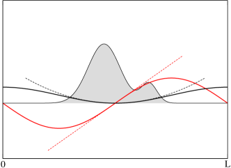
Figure 1: Pictorial representation of the position (red) and spread (black) operators as they are approximated by the Berry-phase formalism when working in periodic poundary conditions.

These equations can be directly compared to the elementary textbook definitions of the position and quadratic spread for a square-integrable electronic state in one dimension (i.e. without PBC, the superscript $F$ stays for “free-space”):

$$\int_{-\infty}^{\infty}\rho(x)(x-\bar{x}^{F})dx=0$$ (8a)

$$\Omega^{F}=\int_{-\infty}^{\infty}\rho(x)(x-\bar{x}^{F})^{2}dx$$ (8b)

The resemblance is indeed striking, the only difference being the replacement of the $x$ and $x^{2}$ operators with trigonometric functions that are periodic on the cell. This relationship between the (polynomial) free-space operators and the (trigonometric) PBC ones is made evident in Fig. 1, where they are plotted together in order to show their close matching in a region surrounding the localized state. Indeed, by a Taylor expansion one obtains:

$$\Big{(}\frac{L}{2\pi}\Big{)}\sin(\frac{2\pi}{L}x)\sim x-\Big{(}\frac{2\pi}{L}\Big{)}^{2}\frac{x^{3}}{3!}+...$$

$$\Big{(}\frac{L}{2\pi}\Big{)}^{2}\big{[}2-2\cos(\frac{2\pi}{L}x)\big{]}\sim x^{2}-2\Big{(}\frac{2\pi}{L}\Big{)}^{2}\frac{x^{4}}{4!}+...$$

Thus, we arrived from a different starting point at the same $\mathcal{O}(L^{-2})$ convergence of the position and spread, which has already been discussed in the literature mv ; puma . It is particularly clear from this derivation that the intrinsic property of the periodic lattice and the localized state are by no means responsible for the slow convergence, which is instead determined exclusively by the mathematical form of the PBC position operator.

To end this section, we note that Eq. 7a alone is not sufficient to define the center $\bar{x}$, since also $\bar{x}+\frac{L}{2}$ satisfies the same requirement. In the context of Equations 7a and 7b, a correct definition of $\bar{x}$ can be given as the points in the lattice which minimize Eq. 7b (it is easy to show that this definition is identical to the standard one in Eq. 6). Interestingly, from this point of view the position $\bar{x}$ can be thought of as an internal parameter of the formalism, which is implicit in the definition of the spread.

IV Correction scheme

Since we are working with Wannier functions which are expected to be well localized in space (as the 1D state depicted in Fig. 1), there is actually no need to insist on using the PBC formulas for calculating Wannier centers. One could argue here that our “Wannier functions” are formally still periodic (although represented on a large BvK supercell), and since their Hilbert space is defined within PBC, only the action of PBC-allowed operators is justified on them. Actually, another point of view can be used. We recall that true Wannier functions are continuous functions in the full 3D (reciprocal) $q$-space. The mean value of a local operator $V(\mathbf{r})$ in real space can be written

$$\langle w_{n}|V|w_{n}\rangle=\int_{All-space}|w_{n}(\mathbf{r})|^{2}V(\mathbf{r})d\mathbf{r}$$ (9)

or, equivalently in $q$-space ($\tilde{\rho}_{n}(\mathbf{q})$ is the continuous Fourier transform of the Wannier density $\rho_{n}(\mathbf{r})=|w_{n}(\mathbf{r})|^{2}$):

$$\langle w_{n}|V|w_{n}\rangle=\int_{|\mathbf{q}|<E_{cut}}\tilde{V}(\mathbf{q})^{*}\tilde{\rho}_{n}(\mathbf{q})d\mathbf{q}$$ (10)

If the Wannier function is localized (i.e. zero beyond a given distance from its center), the integral in Eq. 9 can be limited to a finite region of space, for example a cubic box centered around the region where the Wannier density is nonzero. The $q$-space integral in Eq. 10 can then be recast to a sum over a discrete set of reciprocal space vectors, which is also finite because of the plane-wave cut off, and the result is still exact.

If the integration box is chosen to be smaller than the region where the Wannier density is nonzero, then the reciprocal-space sum carries an error which is due to the overlap between the tails of the Wannier functions and their (artificially) repeated images. This overlap depends on the decay properties of the localized state, and in particular it goes exponentially to zero for increasing integration box size whenever $|w_{n}\rangle$ is exponentially localized.

In a standard DFT simulation of a periodic crystal, the discrete set of reciprocal-space Wannier function coefficients are defined by Eq. 1, and converge to their thermodynamic limit as soon as the total charge density is converged. Then, the only effect of a further refinement of the $k$-points mesh is an increase in the BvK cell volume, which leads to the progressive reduction of the overlap term discussed above. Therefore, assuming exponential decay for the Wannier functions, our technique allows for an exponential convergence of the calculated expectation value of any free-space operator. The natural “bounding box” for the integration domain in real space is, for a general lattice, a Wigner-Seitz BvK cell aligned on the Wannier center. With this choice, the discrete Fourier representation of a given local free-space operator (we use here again the standard conventions for normalizations and Fourier transforms) is:

$$\tilde{V}(\mathbf{b})=\frac{1}{V_{BvK}}\int_{Wigner-Seitz}e^{-i\mathbf{b.r}}V(\mathbf{r})d\mathbf{r},$$

and the expectation value is simply given as

$$\langle w_{n}|V|w_{n}\rangle=V_{BvK}\sum_{\mathbf{b}}\tilde{V}^{*}(\mathbf{b})\tilde{\rho}_{n}(\mathbf{b})$$

Starting from a well-localized set of Wannier functions we can now define a “refined” spread operator $\Omega^{\prime}=\sum_{n}\Omega_{n}^{\prime}$, where the contribution from the individual WF is:

$$\Omega_{n}^{\prime}=\int_{Wigner-Seitz}|\mathbf{r}-\bar{\mathbf{r}}_{n}^{\prime}|^{2}\rho_{n}(\mathbf{r})d\mathbf{r}.$$

The $b$-space expression for this formula can be derived starting from the Fourier series of a parabola in a one dimensional box:

$$\frac{1}{L}\int_{-\frac{L}{2}}^{\frac{L}{2}}\cos(\frac{2\pi k}{L}x)x^{2}dx=\Big{(}\frac{L}{2\pi}\Big{)}^{2}\,\frac{2(-1)^{k}}{k^{2}}\qquad(k>0)$$

$$\frac{1}{L}\int_{-\frac{L}{2}}^{\frac{L}{2}}x^{2}dx=\frac{L^{2}}{4},$$

and is readily generalized to three dimensions using the same set of vectors and weights {$\mathbf{b}_{i},\bar{\mathrm{w}}_{i}$} introduced in Section 2:

$$\Omega_{n}^{\prime}=2V_{BvK}\sum_{i,k>0}\bar{\mathrm{w}}_{i}\mathrm{Re}\Big{[}\frac{2(-1)^{k}}{k^{2}}\,e^{ik\mathbf{b}_{i}.\bar{\mathbf{r}}_{n}^{\prime}}\,\tilde{\rho}_{n}(k\mathbf{b}_{i})\Big{]}+$$

$$+\frac{\pi^{2}}{3}\sum_{i}\bar{\mathrm{w}}_{i}$$ (11)

The “refined” position $\bar{\mathbf{r}}_{n}^{\prime}$ which appears in Eq. 11 is then again an internal parameter, which is defined by the minimum of $\Omega_{n}^{\prime}$ for a given $\tilde{\rho}_{n}$ (see the discussion at the end of Section 3). By taking the gradient of $\Omega_{n}^{\prime}$ with respect to $\bar{\mathbf{r}}_{n}^{\prime}$ one obtains that, at the minimum, the integral:

$$\Delta\mathbf{r}_{n}=\int_{Wigner-Seitz}(\mathbf{r}-\bar{\mathbf{r}}_{n}^{\prime})\rho_{n}(\mathbf{r})d\mathbf{r}$$

vanishes. Consistently with the definition of the spread, this condition has to be enforced in reciprocal space, where this integral becomes:

$$\Delta\mathbf{r}_{n}=-2V_{BvK}\sum_{i,k>0}\bar{\mathrm{w}}_{i}\mathbf{b}_{i}\mathrm{Re}\,\Big{[}i\frac{(-1)^{k}}{k}e^{ik\mathbf{b}_{i}.\bar{\mathbf{r}}_{n}^{\prime}}\tilde{\rho}_{n}(k\mathbf{b}_{i})\Big{]},$$ (12)

The stationary point can be obtained iteratively starting from a set of maximally localized Wannier functions and unrefined centers, by updating at every iteration $\bar{\mathbf{r}}_{n}^{\prime}$ through the addition of $\Delta\mathbf{r}_{n}$ as calculated in Eq. 12 until convergence is reached. If the Wannier function is exactly zero in a region surrounding the boundary of the Wigner-Seitz cell, one iteration is sufficient to provide the exact value of the center, while for less converged cases up to ten iterations may be necessary to achieve machine precision. These iterations have anyway negligible cost, since the Fourier transform of the Wannier function on the BvK cell has to be evaluated only at the beginning (twice for each Wannier function to get the density in reciprocal space).

Both expressions $\Omega$ and $\Omega^{\prime}$ are in fact particular cases of a class of localization criteria which rely on individual Wannier densities only, through some generalized spread functional $S$:

$$\Omega=\sum_{n}S[\rho_{n}]$$

A similar generalised, density-dependent spread can be used in practice to explore alternative localization criteria, like e.g. the maximal Coulomb self-repulsion of Edmiston and Ruedenberg edmiston , or the orbital self-interaction as defined by Perdew and Zunger perdew . An article comparing such alternatives is under preparation inprep .

Since the present free-space-like expressions for position and spread are more accurate than those derived in the first part of this work, one could wonder why we did not use them from the beginning. The reason is exclusively related to computational efficiency. In Eqns. 3 the localization algorithm involves operations on small $J\times J$ matrices only, where $J$ is the number of bands in the primitive cell (the computationally intensive calculation of the $M^{(\mathbf{k},\mathbf{b}_{i})}$ matrices has to be performed only once at the beginning of the iterative minimization). If, instead, the refined spread (or one of the alternative localization criteria discussed above) is used directly for localizing the Wannier functions, several Fourier transforms on the full Wannier (BvK) grid are required for each iteration, at a substantially higher cost. This expensive procedure is anyway not necessary for the scope of the present work, since the actual set of Wannier wavefunctions obtained from one localization method or the other coincide in practice to a high degree of accuracy hydrogen (in particular, the decay properties are expected to be very similar). Therefore, we find it most convenient to use this refinement step in a one-shot fashion once a set of maximally localized Wannier functions is obtained within the more efficient localization functional (Eqns. 3).

V Numerical tests

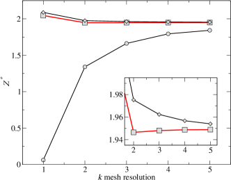
Figure 2: Convergence of the Born effective charge $Z^{*}$ of oxygen in MgO as computed using the sum of unrefined Wannier centers (Eq. 3a, circles), the Berry-phase approach (Eq. 13, diamonds) and our new scheme (Eq. 11, squares). The blow-up in the inset shows the improvement of our method with respect to the Berry-phase approach.

To demonstrate the effectiveness of our method we have chosen two examples which have been extensively studied in the literature: (i) the dynamical Born effective charge of oxygen atoms in rocksalt MgO, and (ii) the spontaneous polarization of the ferroelectric, tetragonally distorted phase of KNbO₃. Our calculations were performed within the local density approximation perdew , by using norm-conserving Troullier and Martins tm pseudopotentials in the Kleinman and Bylander kb form. A non-linear core correction louie was adopted for the Mg pseudopotential, while the K pseudopotential was generated in the $4s^{0}$ ionized configuration with the semicore $3s,3p$ orbitals included in the valence. We used the experimental lattice constants and atomic positions ($a_{0}$=7.96 a.u. for MgO mgoexp , and the structural data for KNbO₃ from Ref. baldoknbo3, ). We expanded the electronic ground state on a plane-wave basis up to a cutoff of 70 Ry. The BZ sampling was performed with $\Gamma$-centered simple cubic (orthorombic) grids in reciprocal space for MgO (KNbO₃), by taking into account the time-reversal symmetry only.

We will compare the results as a function of $k$-mesh resolution for three different methods for calculating the polarization: (i) the sum of Wannier centers as obtained by Eq. 3a; (ii) the sum of refined Wannier centers as described in the previous section; (iii) the Berry-phase approach. We note that the Berry-phase result can be readily obtained from the quantities that are already available in the localization formalism:

$$\mathbf{r}_{Berry}=-\frac{1}{N}\sum_{i}\bar{\mathrm{w}}_{i}\mathbf{b}_{i}\sum_{\mathbf{k}}\mathrm{Im}\ln\det M^{(\mathbf{k,b}_{i})}.$$ (13)

V.1 MgO

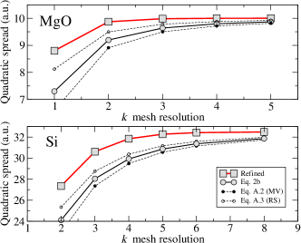
Figure 3: Convergence of the total spread in the case of MgO and Si. The improvement provided by the refined value (Eq. 11, red line and squares) with respect to the standard “trigonometric” spread (Eq. 3b, black line and circles) is apparent. We provide for comparison the alternative spreads discussed in the Appendix, which are also based on the same trigonometric kernel and show similar, slow convergence properties.

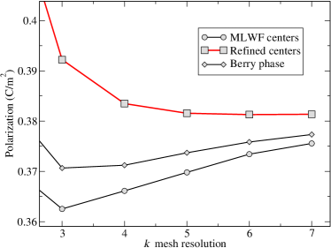
Figure 4: Convergence of the spontaneous polarization of the (tetragonal) ferroelectric phase of KNbO₃, as computed using the sum of unrefined Wannier centers (Eq. 3a, circles), the Berry-phase approach (Eq. 13, diamonds) and our new scheme (Eq. 11, squares).

The dynamical Born effective charge ($Z^{*}$) of oxygen was calculated by the finite-difference method, i.e. by considering the difference in total polarization between the ideal centrosymmetric ground state and an atomic configuration where the oxygen sublattice was displaced by 1% of the cubic lattice constant along the $x$ direction. The atomic coordinates were prepared in such a way that, in the ideal lattice, the O atom sits at the origin, and in this case the electronic contribution to the polarization is exactly zero modulo a polarization quantum (all four Wannier functions are symmetrical about the O in this case). We compare in Fig. 2 the resulting value for $Z^{*}$ as calculated by the three different methods (i-iii). The results clearly show that the sum of the unrefined Wannier centers can be very inaccurate, and even for the finest mesh the error is still large. MgO is probably a very unfortunate case in that each $sp^{3}$-like Wannier function has a strongly asymmetric shape, and the errors in the individual centers do not cancel out efficiently in the strained configuration, so that the total polarization carries an important deviation from the exact value. The Berry-phase calculation is a much better estimate, but in the inset it can be seen that the convergence is still relatively slow. As we explained in the preceding sections, it was already shown that the Berry-phase result converges only as $\mathcal{O}(L^{-2})$, i.e. it shares the same asymptotic behaviour as the sum of the unrefined Wannier centers (albeit with a quite different prefactor in this particular case). The sum of the refined Wannier centers instead shows an extremely fast convergence, and gives a very accurate result already for a $2\times 2\times 2$ mesh. The value of $Z^{*}$ we obtain is -1.95, which is in excellent agreement with previous experimental and theoretical investigations pumaprl .

To complement our methodological test, we calculated also the refined value for the total quadratic spread as a function of $k$-mesh resolution, and the results are reported in Fig. 3. It is clear that this quantity shares the same, excellent, convergence properties as the position operator (upper panel). In the lower panel of the same figure we report for comparison the results of an analogous calculation of the total spread in bulk silicon. The convergence is slower than in MgO, as can be expected from the very different character of this covalent compound as compared to the highly ionic magnesium oxide, but the benefit that can be obtained through the use of the more accurate free-space definition of the spread is still very clear. The “unrefined” value of the spread is also compared to the alternative, very similar prescriptions discussed in the Appendix.

V.2 KNbO₃

We present in Fig. 4 our results for the spontaneous polarization of KNbO₃. The sum of the unrefined Wannier centers is less inaccurate in this case, and is fairly close to the values obtained within the Berry phase formalism. The sum of the refined centers has, again, much better convergence properties than the two traditional methods. By increasing the mesh from $6\times 6\times 6$ to $7\times 7\times 7$ the value of the spontaneous polarization increases by 0.02 %, while within the same $7\times 7\times 7$ mesh the traditional techniques carry an error which is two orders of magnitude higher. Extrapolating the $\mathcal{O}(L^{-2})$ trend one can guess that $\sim 70$ $k$-points along the reciprocal space stripes kingsmith would be needed to achieve similar accuracy within the Berry-phase formalism. The final value we obtain, 0.38 C/m², compares very well with experimental data and previous theoretical investigations baldoknbo3 ; dovesiknbo3 ; restaknbo3 ; vanknbo3 .

VI Conclusions

In conclusion, we have derived a simple and general formalism for the computation of maximally localized Wannier functions. We provide an intuitive picture of the convergence properties of this scheme and similar ones, relating them to the Taylor expansion of elementary trigonometric functions. We show that the convergence can be dramatically improved by a simple strategy based on the exponential localization of the Wannier functions in insulating materials. We expect our scheme to open the way to both accurate and efficient calculations of polarization properties in a wide range of physical systems, making the expensive linear-response approach or the relatively cumbersome non-self consistent calculation of “stripes” in reciprocal space unnecessary.

As a final remark, we note that the Wannier function-based theory of polarization is becoming increasingly important especially in disordered systems, where not only the global polarization but also the local bonding properties and dipole moments may be interesting to follow during, e.g. a molecular dynamics simulation sharma . In these applications the improved accuracy provided by our method could be an extremely valuable tool.

We wish to thank David Vanderbilt for insightful comments on the manuscript. This work was supported by the National Science Foundation’s Division of Materials Research through the Information Technology Research program, grant number DMR-0312407, and made use of MRL Central Facilities supported by the National Science Foundation under award No. DMR-0080034

*

Appendix A Decomposition into invariant, off-diagonal and diagonal parts

The form 2b for the spread functional was chosen mainly because of its simplicity, and because it allows for a direct interpretation as the integral of the Wannier density multiplied by a real function on the BvK cell (see the discussion in Sec. 3). Unfortunately this expression does not lead to an elegant separation into invariant and non-invariant parts. However, this issue is readily solved by choosing an alternative definition of the spread:

$$\Omega_{MV}=\Big{(}\frac{L}{2\pi}\Big{)}^{2}(1-|z|^{2}),$$ (14)

which coincides with the $\Gamma$-point prescription of MV and which does allow for an exact separation of the invariant part. This choice still allows for the simple interpretation based on cosine-like functions. If we define a function of $x_{0}$:

$$f(x_{0})=\int_{0}^{L}\rho(x)\cos[\frac{2\pi}{L}(x-x_{0})]dx$$ (15)

it is clear that when $x_{0}$ maximizes $f$, $x_{0}$ is automatically the Wannier center of Eq. 2a. Both expressions for the spread ($\Omega$ as in Eq. 2b and $\Omega_{MV}$ discussed here) are consistent with the same value of $x_{0}$ at the minimum:

$$\Omega=\Big{(}\frac{L}{2\pi}\Big{)}^{2}\min_{x_{0}}2[1-f(x_{0})]$$

$$\Omega_{MV}=\Big{(}\frac{L}{2\pi}\Big{)}^{2}\min_{x_{0}}[1-f^{2}(x_{0})]$$

Moving on to 3D, the operational definition of the spread becomes:

$$\Omega_{MV}=\sum_{n}\sum_{i}\bar{\mathrm{w}}_{i}\,\big{(}1-|z_{n}^{(i)}|^{2}\big{)},$$

where it is easy to see that $z_{n}^{(i)}$ are nothing other than the matrix elements indicated as $X_{nn}$, $Y_{nn}$, $Z_{nn}$ in MV.

Now, “folding” this expression in $k$-space leads to a formula which is similar to Eq. 3b:

$$\Omega=\sum_{n}\sum_{i}\bar{\mathrm{w}}_{i}\,\big{(}1-\Big{|}\frac{1}{N}\sum_{\mathbf{k}}M^{(\mathbf{k,b}_{i})}_{nn}\Big{|}^{2}\big{)}$$

Thinking in terms of the big BvK cell, this can be written equivalently as:

$$\Omega=\frac{1}{N}\sum_{i}\bar{\mathrm{w}}_{i}(NJ-\sum_{\mathbf{R},n}|\langle\mathbf{R}n|e^{-i\mathbf{b}_{i}.\mathbf{r}}|\mathbf{R}n\rangle|^{2}),$$

where the leading factor $1/N$ gives the spread per primitive cell, and the same notations as MV for the $n$-th Wannier function at the $\mathbf{R}$ site, $|\mathbf{R}n\rangle$ are used. From this expression it is clear how to construct an obvious invariant quantity, $\Omega_{I}$ ($J$ is the number of bands in the primitive cell):

$$\Omega_{I}=\frac{1}{N}\sum_{i}\bar{\mathrm{w}}_{i}(NJ-\sum_{\mathbf{R}\mathbf{R}^{\prime},nm}|\langle\mathbf{R}n|e^{-i\mathbf{b}_{i}.\mathbf{r}}|\mathbf{R}^{\prime}m\rangle|^{2}),$$

and what remains to do is to “unfold” this formula in $k$-space. A first simplification is trivial:

$$\Omega_{I}=\sum_{i}\bar{\mathrm{w}}_{i}(J-\sum_{\mathbf{R},nm}|\langle\mathbf{R}n|e^{-i\mathbf{b}_{i}.\mathbf{r}}|\mathbf{0}m\rangle|^{2}).$$

A second simplification is obtained by reversing the formula between Eq. 5 and 6 of MV, leading to:

$$\Omega_{I}=\sum_{i}\bar{\mathrm{w}}_{i}(J-\sum_{\mathbf{R},nm}\Big{|}\frac{1}{N}\sum_{\mathbf{k}}e^{i\mathbf{k.R}}\langle u_{n\mathbf{k}}|e^{-i\mathbf{b}_{i}.\mathbf{r}}|u_{m\mathbf{k+b}}\rangle\Big{|}^{2}).$$

By writing explicitly $|z|^{2}=z^{*}z$ and noticing that

$$\sum_{\mathbf{R}}e^{i\mathbf{(k-k^{\prime}).R}}=N\delta_{\mathbf{k,k^{\prime}}},$$

we obtain the final expression in $k$-space:

$$\Omega_{I}=\sum_{i}\bar{\mathrm{w}}_{i}(J-\sum_{mn}\frac{1}{N}\sum_{\mathbf{k}}\Big{|}M^{(\mathbf{k,b}_{i})}_{nm}\Big{|}^{2}),$$ (16)

which is exactly Eq. 34 of the MV paper.

It is interesting to work out the remaining terms, $\Omega_{D}$ and $\Omega_{OD}$, which are indicated as “diagonal” and “off-diagonal” parts in MV (we recall that $\Omega_{D}$ vanishes for a centrosymmetric system mv ). The easiest way is to first solve the expression for

$$\Omega_{MV}-\Omega_{D}=\sum_{i}\bar{\mathrm{w}}_{i}(J-\sum_{\mathbf{R},n}|\langle\mathbf{R}n|e^{-i\mathbf{b}_{i}.\mathbf{r}}|\mathbf{0}n\rangle|^{2}).$$

By using an analogous algebra we readily arrive at the formula in $k$-space:

$$\Omega_{MV}-\Omega_{D}=\sum_{i}\bar{\mathrm{w}}_{i}(J-\sum_{n}\frac{1}{N}\sum_{\mathbf{k}}\Big{|}M^{(\mathbf{k,b}_{i})}_{nn}\Big{|}^{2}),$$

from which it is very easy to evaluate $\Omega_{OD}$:

$$\Omega_{OD}=\sum_{i}\bar{\mathrm{w}}_{i}\sum_{m\neq n}\frac{1}{N}\sum_{\mathbf{k}}\Big{|}M^{(\mathbf{k,b}_{i})}_{mn}\Big{|}^{2}.$$

This means that $\Omega_{D}$ is given by the following difference:

$$\Omega_{D}=\sum_{i,n}\bar{\mathrm{w}}_{i}\big{(}\Big{|}\frac{1}{N}\sum_{\mathbf{k}}M^{(\mathbf{k,b}_{i})}_{nn}\Big{|}^{2}-\frac{1}{N}\sum_{\mathbf{k}}\Big{|}M^{(\mathbf{k,b}_{i})}_{nn}\Big{|}^{2}\big{)}.$$

Comparing this formalism with the MV one, it is clear that $\Omega_{I}$ and $\Omega_{OD}$ are identical, while the terms $\Omega$ and $\Omega_{D}$ differ. This derivation provide in a certain sense a “unification” of the two, formerly distinct, MV prescriptions for the $\Gamma$-point case and in $k$-space. The gradients with respect to unitary rotations of the Bloch orbitals are simply given by setting $C=z$ (instead of $C=z/|z|$) in Eq. 4.

To complete our discussion, we note that a third form of the one-particle quadratic spread was proposed by Resta and Sorella rs , which leads to yet another operational definition for the localization criterion:

$$\Omega_{RS}=-\sum_{n}\sum_{i}\bar{\mathrm{w}}_{i}\,\ln\,|z_{n}^{(i)}|^{2}.$$

The $k$-space folding of this formula is straightforward, while the gradient is again given by Eq. 4, with $C=z/|z|^{2}$. All functionals $\Omega$, $\Omega_{MV}$ and $\Omega_{RS}$ are identical in the thermodynamic limit. For finite BvK cells they all share the same definition of the Wannier center. The resulting maximally localized Wannier functions themselves are identical in cases where $|z_{n}|$ are equal for all $n=1,...,J$ bands (e.g. bulk Si, centrosymmetric MgO crystal). The numerical value of the spread can differ slightly, because the higher orders in the Taylor expansion are different. Some examples concerning this discrepancy are reported in the main text (see, e.g., Fig. 3).

References

- (1) G. H. Wannier, Phys. Rev. 52, 191 (1937).
- (2) R. M. Martin, Electronic structure: Basic Theory and Practical Methods, Cambridge University Press (2004).
- (3) N. Marzari and D. Vanderbilt, Phys. Rev. B 56, 12847 (1997).
- (4) I. Souza et al., Phys. Rev. B 62, 15505 (2000).
- (5) M. Sharma, Y. Wu and R. Car, Int. J. Quant. Chem. 95, 821 (2003).
- (6) G. Cangiani, A. Baldereschi, M. Posternak and H. Krakauer, Phys. Rev. B 69, 121101(R) (2004).
- (7) P. Fernández, A. Dal Corso and A. Baldereschi, Phys. Rev. B 58, R7480 (1998).
- (8) M. Posternak et al., Phys. Rev. B 65, 184422 (2002).
- (9) Y. Noel et al., Phys. Rev. B 65, 014111 (2001).
- (10) E. Pavarini et al. Phys. Rev. Lett. 92, 176403 (2004).
- (11) S. Fabris et al., Phys. Rev. B 71, 041102 (2005).
- (12) F. Giustino, P. Umari and A. Pasquarello, Phys. Rev. Lett. 91, 267601 (2003).
- (13) K. S. Thygesen, L. B. Hansen and K. W. Jacobsen, Phys. Rev. Lett. 94, 026405 (2005).
- (14) R. D. King-Smith and D. Vanderbilt, Phys. Rev. B 47, 1651 (1993).
- (15) P. Umari and A. Pasquarello Phys. Rev. B 68, 085114 (2003).
- (16) C. Sagui et al., J. Chem. Phys. 120, 4530 (2004).
- (17) J. Bennetto and D. Vanderbilt, Phys. Rev. B 53, 15417 (1996).
- (18) C. M. Zicovich-Wilson et al., J. Chem. Phys. 115, 9708 (2001).
- (19) Ph. Baranek et al., Phys. Rev. B 64, 125102 (2001).
- (20) R. Resta, J. Phys.: Condens. Matter 14, R625 (2002).
- (21) G. Berghold et al., Phys. Rev. B 61, 10040 (2000).
- (22) P. L. Silvestrelli, Phys. Rev. B 59, 9703 (1999).
- (23) L. He and D. Vanderbilt, Phys. Rev. Lett. 86, 5341 (2001).
- (24) R. Resta, Phys. Rev. Lett. 80, 1800 (1998).
- (25) C. Edmiston and K. Ruedenberg, Rev. Mod. Phys. 35, 457 (1963).
- (26) J. P. Perdew and A. Zunger, Phys. Rev. B 23, 5048 (1981).
- (27) M. Stengel and N. A. Spaldin, in preparation.
- (28) N. Troullier and J. L. Martins, Phys. Rev. B 43, 1993 (1991).
- (29) L. Kleinman and D. M. Bylander, Phys. Rev. Lett. 48, 1425 (1982).
- (30) S. G. Louie, S. Froyen and M. L. Cohen, Phys. Rev. B 26, 1738 (1982).
- (31) G. Cappellini et al., J. Phys.: Condens. Matter 12, 3671 (2000).
- (32) R. Resta, M. Posternak and A. Baldereschi, Phys. Rev. Lett. 70, 1010 (1993).
- (33) P. Umari and A. Pasquarello, Phys. Rev. Lett. 89, 157602 (2002).
- (34) S. Dall’Olio, R. Dovesi and R. Resta, Phys. Rev. B 56, 10105 (1997).
- (35) W. Zhong, R. D. King-Smith and D. Vanderbilt, Phys. Rev. Lett. 72, 3618 (1994).
- (36) R. Resta and S. Sorella, Phys. Rev. Lett. 82, 370 (1999).