[

Enhancement of superconducting transition temperature by the additional second neighbor hopping $t^{\prime}$ in the $t$-$J$ model

Abstract

Within the kinetic energy driven superconducting mechanism, the effect of the additional second neighbor hopping $t^{\prime}$ on the superconducting state of the $t$-$J$ model is discussed. It is shown that $t^{\prime}$ plays an important role in enhancing the superconducting transition temperature of the $t$-$J$ model. It is also shown that the superconducting-state of cuprate superconductors is the conventional Bardeen-Cooper-Schrieffer like, so that the basic Bardeen-Cooper-Schrieffer formalism is still valid in quantitatively reproducing the doping dependence of the superconducting gap parameter and superconducting transition temperature, and electron spectral function at ($\pi$,0) point, although the pairing mechanism is driven by the kinetic energy by exchanging dressed spin excitations.

]

After intensive investigations over more than a decade, it has now become clear that although the physical properties of cuprate superconductors in the normal-state are fundamentally different from these of the conventional metals [1], the superconducting (SC)-state of cuprate superconductors is still associated with the formation of the electron Cooper pairs [2] as in the conventional superconductors. In the conventional metals, superconductivity results when electrons pair up into Cooper pairs, which is mediated by the interaction of electrons with phonons [3]. As a result, the pairing in the conventional superconductors is always related with an increase in kinetic energy which is overcompensated by the lowering of potential energy [4]. However, it has been argued that the form of the electron Cooper pairs is determined by the need to reduce the frustrated kinetic energy in doped cuprates [5, 6], i.e., the strong frustration of the kinetic energy in the normal-state is partially relieved upon entering the SC-state. By virtue of systematic studies using the nuclear magnetic resonance, and muon spin rotation techniques, particularly the inelastic neutron scattering, it has been well established that the antiferromagnetic (AF) short-range correlation (AFSRC) coexists with the SC-state in the whole SC regime [7, 8], which provide a clear link between the SC pairing mechanism and magnetic excitations. Moreover, it has been shown [9] that although the SC pairing mechanism of cuprate superconductors is beyond the conventional electron-phonon mechanism, the SC-state is the conventional Bardeen-Cooper-Schrieffer (BCS) like [3], so that the basic BCS formalism is still valid in discussions of the electron spectral properties [9].

Very soon after the discovery of superconductivity in doped cuprates, Anderson [10] suggested that the essential physics of doped cuprates is contained in the $t$-$J$ model on a square lattice. This followed from the experiments that cuprate superconductors are doped antiferromagnets, where the common features are the presence of the square lattice CuO₂ planes [1] and a similar phase diagram as a function of the doping concentration [11]. Since then much effort has concentrated on the unusual normal-state and SC mechanism within the $t$-$J$ model [5, 12]. Based on the charge-spin separation (CSS) fermion-spin theory [13], we [14] have developed a kinetic energy driven SC mechanism within the $t$-$J$ model. It is shown [14] that the dressed holons interact occurring directly through the kinetic energy by exchanging the spin excitations, leading to a net attractive force between the dressed holons, then the electron Cooper pairs originating from the dressed holon pairing state are due to the charge-spin recombination, and their condensation reveals the SC ground-state. This SC-state is controlled by both SC gap function and quasiparticle coherence, and the maximal SC transition temperature occurs around the optimal doping, then decreases in both underdoped and overdoped regimes [15]. However, the simple $t$-$J$ model can not be regarded as a comprehensive model for the quantitative comparison with cuprate superconductors. It has been shown [16] from the angle resolved photoemission spectroscopy (ARPES) experiments that although the highest energy filled electron band is well described by the $t$-$J$ model in the direction between the $[0,0]$ point and the $[\pi,\pi]$ point in the momentum space, but both experimental data near $[\pi,0]$ point and overall dispersion may be properly accounted by generalizing the $t$-$J$ model to include the second- and third-nearest neighbors hopping terms $t^{\prime}$ and $t^{\prime\prime}$. Moreover, the experimental analysis [17] shows that the SC transition temperature for different families of cuprate superconductors is strongly correlated with $t^{\prime}$. In this Letter, we discuss the effect of the additional second neighbor hopping $t^{\prime}$ on the SC-state of the $t$-$J$ model within the framework of the kinetic energy driven SC mechanism [14]. Our result shows that the SC-state of cuprate superconductors is the conventional BCS like [3], so that the basic BCS formalism is still valid in quantitatively reproducing the doping dependence of the effective SC gap parameter and SC transition temperature, and electron spectral function at $[\pi,0]$ point, although the pairing mechanism is driven by the kinetic energy by exchanging dressed spin excitations, and other exotic magnetic properties [15] are beyond the BCS theory. Our result also shows that the additional second neighbor hopping $t^{\prime}$ plays an important role in enhancing the SC transition temperature of the $t$-$J$ model and in determining the correct position of the SC quasiparticle peak of the electron spectral function at $[\pi,0]$ point.

We start from the $t$-$t^{\prime}$-$J$ model on a square lattice [10, 16],

$$H = -t\sum_{i\hat{\eta}\sigma}C^{\dagger}_{i\sigma}C_{i+\hat{\eta}\sigma}+t^{\prime}\sum_{i\hat{\tau}\sigma}C^{\dagger}_{i\sigma}C_{i+\hat{\tau}\sigma}+\mu\sum_{i\sigma}C^{\dagger}_{i\sigma}C_{i\sigma}$$ (1)

$$+ J\sum_{i\hat{\eta}}{\bf S}_{i}\cdot{\bf S}_{i+\hat{\eta}},$$ (2)

supplemented by the local constraint $\sum_{\sigma}C^{\dagger}_{i\sigma}C_{i\sigma}\leq 1$ to avoid the double occupancy, where $\hat{\eta}=\pm\hat{x},\pm\hat{y}$, $\hat{\tau}=\pm\hat{x}\pm\hat{y}$, $C^{\dagger}_{i\sigma}$ ($C_{i\sigma}$) is the electron creation (annihilation) operator, ${\bf S}_{i}=C^{\dagger}_{i}{\vec{\sigma}}C_{i}/2$ is spin operator with ${\vec{\sigma}}=(\sigma_{x},\sigma_{y},\sigma_{z})$ as Pauli matrices, and $\mu$ is the chemical potential. The strong electron correlation in the $t$-$t^{\prime}$-$J$ model manifests itself by the electron single occupancy local constraint [10], which can be treated properly in analytical calculations within the CSS fermion-spin theory [13], where the constrained electron operators are decoupled as $C_{i\uparrow}=h^{\dagger}_{i\uparrow}S^{-}_{i}$ and $C_{i\downarrow}=h^{\dagger}_{i\downarrow}S^{+}_{i}$, with the spinful fermion operator $h_{i\sigma}=e^{-i\Phi_{i\sigma}}h_{i}$ describes the charge degree of freedom together with some effects of the spin configuration rearrangements due to the presence of the doped hole itself (dressed holon), while the spin operator $S_{i}$ describes the spin degree of freedom (dressed spin), then the electron local constraint for the single occupancy, $\sum_{\sigma}C^{\dagger}_{i\sigma}C_{i\sigma}=S^{+}_{i}h_{i\uparrow}h^{\dagger}_{i\uparrow}S^{-}_{i}+S^{-}_{i}h_{i\downarrow}h^{\dagger}_{i\downarrow}S^{+}_{i}=h_{i}h^{\dagger}_{i}(S^{+}_{i}S^{-}_{i}+S^{-}_{i}S^{+}_{i})=1-h^{\dagger}_{i}h_{i}\leq 1$, is satisfied in analytical calculations. It has been shown that these dressed holon and spin are gauge invariant [13], and in this sense, they are real and can be interpreted as the physical excitations [12]. Although in common sense $h_{i\sigma}$ is not a real spinful fermion, it behaves like a spinful fermion. In this CSS fermion-spin representation, the low-energy behavior of the $t$-$t^{\prime}$-$J$ model (1) can be expressed as,

$$H = -t\sum_{i\hat{\eta}}(h_{i\uparrow}S^{+}_{i}h^{\dagger}_{i+\hat{\eta}\uparrow}S^{-}_{i+\hat{\eta}}+h_{i\downarrow}S^{-}_{i}h^{\dagger}_{i+\hat{\eta}\downarrow}S^{+}_{i+\hat{\eta}})$$ (3)

$$+ t^{\prime}\sum_{i\hat{\tau}}(h_{i\uparrow}S^{+}_{i}h^{\dagger}_{i+\hat{\tau}\uparrow}S^{-}_{i+\hat{\tau}}+h_{i\downarrow}S^{-}_{i}h^{\dagger}_{i+\hat{\tau}\downarrow}S^{+}_{i+\hat{\tau}})$$ (4)

$$- \mu\sum_{i\sigma}h^{\dagger}_{i\sigma}h_{i\sigma}+J_{{\rm eff}}\sum_{i\hat{\eta}}{\bf S}_{i}\cdot{\bf S}_{i+\hat{\eta}},$$ (5)

with $J_{{\rm eff}}=(1-x)^{2}J$, and $x=\langle h^{\dagger}_{i\sigma}h_{i\sigma}\rangle=\langle h^{\dagger}_{i}h_{i}\rangle$ is the hole doping concentration. As a consequence, the kinetic energy terms in the $t$-$t^{\prime}$-$J$ model have been expressed as the dressed holon-spin interactions, which reflects that even the kinetic energy terms in the $t$-$t^{\prime}$-$J$ Hamiltonian have strong Coulombic contributions due to the restriction of no doubly occupancy of a given site, and therefore dominate the essential physics of doped cuprates.

ARPES measurements [18] show that in the real space the gap function and pairing force have a range of one lattice spacing, which indicates that the order parameter for the electron Cooper pair can be expressed as,

$$\Delta = \langle C^{\dagger}_{i\uparrow}C^{\dagger}_{i+\hat{\eta}\downarrow}-C^{\dagger}_{i\downarrow}C^{\dagger}_{i+\hat{\eta}\uparrow}\rangle$$ (6)

$$= \langle h_{i\uparrow}h_{i+\hat{\eta}\downarrow}S^{+}_{i}S^{-}_{i+\hat{\eta}}-h_{i\downarrow}h_{i+\hat{\eta}\uparrow}S^{-}_{i}S^{+}_{i+\hat{\eta}}\rangle.$$ (7)

In the doped regime without the AF long-range order (AFLRO), the dressed spins form a disordered spin liquid state, where the dressed spin correlation function $\langle S^{+}_{i}S^{-}_{i+\hat{\eta}}\rangle=\langle S^{-}_{i}S^{+}_{i+\hat{\eta}}\rangle$, then the order parameter for the electron Cooper pair in Eq. (3) can be written as $\Delta=-\langle S^{+}_{i}S^{-}_{i+\hat{\eta}}\rangle\Delta_{h}$, with the dressed holon pairing order parameter $\Delta_{h}=\langle h_{i+\hat{\eta}\downarrow}h_{i\uparrow}-h_{i+\hat{\eta}\uparrow}h_{i\downarrow}\rangle$, which shows that the SC order parameter of the electron Cooper pair is related to the dressed holon pairing amplitude, and is proportional to the number of doped holes, and not to the number of electrons. However, in the extreme low doped regime with AFLRO, where the dressed spin correlation function $\langle S^{+}_{i}S^{-}_{i+\hat{\eta}}\rangle\neq\langle S^{-}_{i}S^{+}_{i+\hat{\eta}}\rangle$, then the conduct is disrupted by AFLRO, and therefore there is no mixing of superconductivity and AFLRO [19]. In the case without AFLRO, we [14, 15] have shown within the Eliashberg’s strong coupling theory [20] that the dressed holon-spin interaction can induce the dressed holon pairing state (then the electron Cooper pairing state) by exchanging dressed spin excitations in the higher power of the hole doping concentration. Following our previous discussions based on the $t$-$J$ model [14, 15], the self-consistent equations that satisfied by the full dressed holon diagonal and off-diagonal Green’s functions in the present $t$-$t^{\prime}$-$J$ model are obtained as,

$$g(k) = g^{(0)}(k)$$ (9)

$$+ g^{(0)}(k)[\Sigma^{(h)}_{1}(k)g(k)-\Sigma^{(h)}_{2}(-k)\Im^{\dagger}(k)],$$ (10)

$$\Im^{\dagger}(k) = g^{(0)}(-k)[\Sigma^{(h)}_{1}(-k)\Im^{\dagger}(-k)+\Sigma^{(h)}_{2}(-k)g(k)],$$ (11)

respectively, where the four-vector notation $k=({\bf k},i\omega_{n})$, and the mean-field (MF) dressed holon diagonal Green’s function [13] $g^{(0)-1}(k)=i\omega_{n}-\xi_{{\bf k}}$, with the MF dressed holon excitation spectrum $\xi_{{\bf k}}=Zt\chi_{1}\gamma_{{\bf k}}-Zt^{\prime}\chi_{2}\gamma_{{\bf k}}^{\prime}-\mu$, where $\gamma_{{\bf k}}=(1/Z)\sum_{\hat{\eta}}e^{i{\bf k}\cdot\hat{\eta}}$, $\gamma_{{\bf k}}^{\prime}=(1/Z)\sum_{\hat{\tau}}e^{i{\bf k}\cdot\hat{\tau}}$, $Z$ is the number of the nearest neighbor or second-nearest neighbor sites, the spin correlation functions $\chi_{1}=\langle S_{i}^{+}S_{i+\hat{\eta}}^{-}\rangle$ and $\chi_{2}=\langle S_{i}^{+}S_{i+\hat{\tau}}^{-}\rangle$, while the dressed holon self-energies are obtained from the dressed spin bubble as,

$$\Sigma^{(h)}_{1}(k) = {1\over N^{2}}\sum_{{\bf p,p^{\prime}}}(Zt\gamma_{{\bf p+p^{\prime}+k}}-Zt^{\prime}\gamma_{{\bf p+p^{\prime}+k}}^{\prime})^{2}$$ (13)

$$\times {1\over\beta}\sum_{ip_{m}}g(p+k){1\over\beta}\sum_{ip^{\prime}_{m}}D^{(0)}(p^{\prime})D^{(0)}(p^{\prime}+p),$$ (14)

$$\Sigma^{(h)}_{2}(k) = {1\over N^{2}}\sum_{{\bf p,p^{\prime}}}(Zt\gamma_{{\bf p+p^{\prime}+k}}-Zt^{\prime}\gamma_{{\bf p+p^{\prime}+k}}^{\prime})^{2}$$ (15)

$$\times {1\over\beta}\sum_{ip_{m}}\Im(-p-k){1\over\beta}\sum_{ip^{\prime}_{m}}D^{(0)}(p^{\prime})D^{(0)}(p^{\prime}+p),$$ (16)

where $p=({\bf p},ip_{m})$, $p^{\prime}=({\bf p^{\prime}},ip_{m}^{\prime})$, $N$ is the number of sites, and the MF dressed spin Green’s function [13], $D^{(0)-1}(p)=[(ip_{m})^{2}-\omega_{{\bf p}}^{2}]/B_{{\bf p}}$, with $B_{{\bf p}}=2\lambda_{1}(A_{1}\gamma_{{\bf p}}-A_{2})-\lambda_{2}(2\chi^{z}_{2}\gamma_{{\bf p}}^{\prime}-\chi_{2})$, $\lambda_{1}=2ZJ_{eff}$, $\lambda_{2}=4Z\phi_{2}t^{\prime}$, $A_{1}=\epsilon\chi^{z}_{1}+\chi_{1}/2$, $A_{2}=\chi^{z}_{1}+\epsilon\chi_{1}/2$, $\epsilon=1+2t\phi_{1}/J_{{\rm eff}}$, the dressed holon’s particle-hole parameters $\phi_{1}=\langle h^{\dagger}_{i\sigma}h_{i+\hat{\eta}\sigma}\rangle$ and $\phi_{2}=\langle h^{\dagger}_{i\sigma}h_{i+\hat{\tau}\sigma}\rangle$, the spin correlation functions $\chi^{z}_{1}=\langle S_{i}^{z}S_{i+\hat{\eta}}^{z}\rangle$ and $\chi^{z}_{2}=\langle S_{i}^{z}S_{i+\hat{\tau}}^{z}\rangle$, and the MF dressed spin excitation spectrum,

$$\omega^{2}_{{\bf p}} = \lambda_{1}^{2}[(A_{4}-\alpha\epsilon\chi^{z}_{1}\gamma_{{\bf p}}-{1\over 2Z}\alpha\epsilon\chi_{1})(1-\epsilon\gamma_{{\bf p}})$$ (17)

$$+ {1\over 2}\epsilon(A_{3}-{1\over 2}\alpha\chi^{z}_{1}-\alpha\chi_{1}\gamma_{{\bf p}})(\epsilon-\gamma_{{\bf p}})]$$ (18)

$$+ \lambda_{2}^{2}[\alpha(\chi^{z}_{2}\gamma_{{\bf p}}^{\prime}-{3\over 2Z}\chi_{2})\gamma_{{\bf p}}^{\prime}+{1\over 2}(A_{5}-{1\over 2}\alpha\chi^{z}_{2})]$$ (19)

$$+ \lambda_{1}\lambda_{2}[\alpha\chi^{z}_{1}(1-\epsilon\gamma_{{\bf p}})\gamma_{{\bf p}}^{\prime}+{1\over 2}\alpha(\chi_{1}\gamma_{{\bf p}}^{\prime}-C_{3})(\epsilon-\gamma_{{\bf p}})$$ (20)

$$+ \alpha\gamma_{{\bf p}}^{\prime}(C^{z}_{3}-\epsilon\chi^{z}_{2}\gamma_{{\bf p}})-{1\over 2}\alpha\epsilon(C_{3}-\chi_{2}\gamma_{{\bf p}})],$$ (21)

with $A_{3}=\alpha C_{1}+(1-\alpha)/(2Z)$, $A_{4}=\alpha C^{z}_{1}+(1-\alpha)/(4Z)$, $A_{5}=\alpha C_{2}+(1-\alpha)/(2Z)$, and the spin correlation functions $C_{1}=(1/Z^{2})\sum_{\hat{\eta},\hat{\eta^{\prime}}}\langle S_{i+\hat{\eta}}^{+}S_{i+\hat{\eta^{\prime}}}^{-}\rangle$, $C^{z}_{1}=(1/Z^{2})\sum_{\hat{\eta},\hat{\eta^{\prime}}}\langle S_{i+\hat{\eta}}^{z}S_{i+\hat{\eta^{\prime}}}^{z}\rangle$, $C_{2}=(1/Z^{2})\sum_{\hat{\tau},\hat{\tau^{\prime}}}\langle S_{i+\hat{\tau}}^{+}S_{i+\hat{\tau^{\prime}}}^{-}\rangle$, $C_{3}=(1/Z)\sum_{\hat{\tau}}\langle S_{i+\hat{\eta}}^{+}S_{i+\hat{\tau}}^{-}\rangle$, and $C^{z}_{3}=(1/Z)\sum_{\hat{\tau}}\langle S_{i+\hat{\eta}}^{z}S_{i+\hat{\tau}}^{z}\rangle$. In order to satisfy the sum rule of the correlation function $\langle S^{+}_{i}S^{-}_{i}\rangle=1/2$ in the case without AFLRO, the important decoupling parameter $\alpha$ has been introduced in the MF calculation [14, 21], which can be regarded as the vertex correction.

The self-energy function $\Sigma^{(h)}_{2}(k)$ describes the effective dressed holon gap function, since both doping and temperature dependence of the pairing force and dressed holon gap function have been incorporated into $\Sigma^{(h)}_{2}(k)$, while the self-energy function $\Sigma^{(h)}_{1}(k)$ renormalizes the MF dressed holon spectrum, and therefore it describes the quasiparticle coherence. Moreover, $\Sigma^{(h)}_{2}(k)$ is an even function of $i\omega_{n}$, while $\Sigma^{(h)}_{1}(k)$ is not. For the convenience, $\Sigma^{(h)}_{1}(k)$ can be broken up into its symmetric and antisymmetric parts as, $\Sigma^{(h)}_{1}(k)=\Sigma^{(h)}_{1e}(k)+i\omega_{n}\Sigma^{(h)}_{1o}(k)$, then both $\Sigma^{(h)}_{1e}(k)$ and $\Sigma^{(h)}_{1o}(k)$ are even functions of $i\omega_{n}$. In this case, the quasiparticle coherent weight can be defined as $Z^{-1}_{F}(k)=1-\Sigma^{(h)}_{1o}(k)$. As in the conventional superconductor [20], the retarded function ${\rm Re}\Sigma^{(h)}_{1e}(k)$ is a constant, independent of (${\bf k},\omega$), and it just renormalizes the chemical potential, therefore it can be dropped. Furthermore, we only study the static limit of the effective dressed holon gap function and quasiparticle coherent weight, i.e., $\Sigma^{(h)}_{2}(k)=\bar{\Delta}_{h}({\bf k})$, and $Z^{-1}_{F}({\bf k})=1-\Sigma^{(h)}_{1o}({\bf k})$. Although $Z_{F}({\bf k})$ still is a function of ${\bf k}$, the wave vector dependence is unimportant, since everything happens at the electron Fermi surface. As in the previous discussions within the $t$-$J$ model [15], the special wave vector can be estimated qualitatively from the electron momentum distribution as ${\bf k}_{0}={\bf k_{A}}-{\bf k_{F}}$ with ${\bf k_{A}}=[\pi,\pi]$ and ${\bf k_{F}}\approx[(1-x)\pi/2,(1-x)\pi/2]$, which guarantees $Z_{F}=Z_{F}({\bf k}_{0})$ near the electron Fermi surface. In this case, the dressed holon diagonal and off-diagonal Green’s functions in Eqs. (4a) and (4b) can be expressed explicitly as,

$$g(k) = Z_{F}{U^{2}_{h{\bf k}}\over i\omega_{n}-E_{h{\bf k}}}+Z_{F}{V^{2}_{h{\bf k}}\over i\omega_{n}+E_{h{\bf k}}},$$ (23)

$$\Im^{\dagger}(k) = -Z_{F}{\bar{\Delta}_{hZ}({\bf k})\over 2E_{h{\bf k}}}\left({1\over i\omega_{n}-E_{h{\bf k}}}-{1\over i\omega_{n}+E_{h{\bf k}}}\right),$$ (24)

with the dressed holon quasiparticle coherence factors $U^{2}_{h{\bf k}}=(1+\bar{\xi_{{\bf k}}}/E_{h{\bf k}})/2$ and $V^{2}_{h{\bf k}}=(1-\bar{\xi_{{\bf k}}}/E_{h{\bf k}})/2$, $\bar{\xi_{{\bf k}}}=Z_{F}\xi_{{\bf k}}$, $\bar{\Delta}_{hZ}({\bf k})=Z_{F}\bar{\Delta}_{h}({\bf k})$, and the dressed holon quasiparticle spectrum $E_{h{\bf k}}=\sqrt{\bar{\xi^{2}_{{\bf k}}}+\mid\bar{\Delta}_{hZ}({\bf k})\mid^{2}}$.

Experimentally, some results seem consistent with an s-wave pairing [22], while other measurements gave the evidence in favor of the d-wave pairing [23, 2]. These experiments reflect a fact that the d-wave gap function $\propto{\rm k}^{2}_{x}-{\rm k}^{2}_{y}$ belongs to the same representation $\Gamma_{1}$ of the orthorhombic crystal group as does s-wave gap function $\propto{\rm k}^{2}_{x}+{\rm k}^{2}_{y}$. Within the $t$-$J$ model, we [15] have shown that the electron Cooper pairs have a dominated d-wave symmetry over a wide range of the doping concentration, around the optimal doping. To make the discussion simpler, we only consider the d-wave case, i.e., $\bar{\Delta}_{hZ}({\bf k})=\bar{\Delta}_{hZ}\gamma^{(d)}_{{\bf k}}$, with $\gamma^{(d)}_{{\bf k}}=({\rm cos}k_{x}-{\rm cos}k_{y})/2$. In this case, the dressed holon effective gap parameter and quasiparticle coherent weight in Eqs. (5a) and (5b) satisfy following two equations,

$$1 ={1\over N^{3}}\sum_{{\bf k,q,p}}(Zt\gamma_{{\bf k+q}}-Zt^{\prime}\gamma_{{\bf k+q}}^{\prime})^{2}\gamma^{(d)}_{{\bf k-p+q}}\gamma^{(d)}_{{\bf k}}{Z^{2}_{F}\over E_{h{\bf k}}}{B_{{\bf q}}B_{{\bf p}}\over\omega_{{\bf q}}\omega_{{\bf p}}}$$ (26)

$$\times \left({F^{(1)}_{1}({\bf k,q,p})\over(\omega_{{\bf p}}-\omega_{{\bf q}})^{2}-E^{2}_{h{\bf k}}}-{F^{(2)}_{1}({\bf k,q,p})\over(\omega_{{\bf p}}+\omega_{{\bf q}})^{2}-E^{2}_{h{\bf k}}}\right),$$ (27)

$$Z^{-1}_{F} =1+{1\over N^{2}}\sum_{{\bf q,p}}(Zt\gamma_{{\bf p+k_{0}}}-Zt^{\prime}\gamma_{{\bf p+k_{0}}}^{\prime})^{2}Z_{F}{B_{{\bf q}}B_{{\bf p}}\over 4\omega_{{\bf q}}\omega_{{\bf p}}}$$ (28)

$$\times \left({F^{(1)}_{2}({\bf q,p})\over(\omega_{{\bf p}}-\omega_{{\bf q}}-E_{h{\bf p-q+k_{0}}})^{2}}+{F^{(2)}_{2}({\bf q,p})\over(\omega_{{\bf p}}-\omega_{{\bf q}}+E_{h{\bf p-q+k_{0}}})^{2}}\right.$$ (29)

$$+ \left.{F^{(3)}_{2}({\bf q,p})\over(\omega_{{\bf p}}+\omega_{{\bf q}}-E_{h{\bf p-q+k_{0}}})^{2}}+{F^{(4)}_{2}({\bf q,p})\over(\omega_{{\bf p}}+\omega_{{\bf q}}+E_{h{\bf p-q+k_{0}}})^{2}}\right),$$ (30)

respectively, where $F^{(1)}_{1}({\bf k,q,p})=(\omega_{{\bf p}}-\omega_{{\bf q}})[n_{B}(\omega_{{\bf q}})-n_{B}(\omega_{{\bf p}})][1-2n_{F}(E_{h{\bf k}})]+E_{h{\bf k}}[n_{B}(\omega_{{\bf p}})n_{B}(-\omega_{{\bf q}})+n_{B}(\omega_{{\bf q}})n_{B}(-\omega_{{\bf p}})]$, $F^{(2)}_{1}({\bf k,q,p})=(\omega_{{\bf p}}+\omega_{{\bf q}})[n_{B}(-\omega_{{\bf p}})-n_{B}(\omega_{{\bf q}})][1-2n_{F}(E_{h{\bf k}})]+E_{h{\bf k}}[n_{B}(\omega_{{\bf p}})n_{B}(\omega_{{\bf q}})+n_{B}(-\omega_{{\bf p}})n_{B}(-\omega_{{\bf q}})]$, $F^{(1)}_{2}({\bf q,p})=n_{F}(E_{h{\bf p-q+k_{0}}})[n_{B}(\omega_{{\bf q}})-n_{B}(\omega_{{\bf p}})]-n_{B}(\omega_{{\bf p}})n_{B}(-\omega_{{\bf q}})$, $F^{(2)}_{2}({\bf q,p})=n_{F}(E_{h{\bf p-q+k_{0}}})[n_{B}(\omega_{{\bf p}})-n_{B}(\omega_{{\bf q}})]-n_{B}(\omega_{{\bf q}})n_{B}(-\omega_{{\bf p}})$, $F^{(3)}_{2}({\bf q,p})=n_{F}(E_{h{\bf p-q+k_{0}}})[n_{B}(\omega_{{\bf q}})-n_{B}(-\omega_{{\bf p}})]+n_{B}(\omega_{{\bf p}})n_{B}(\omega_{{\bf q}})$, and $F^{(4)}_{2}({\bf q,p})=n_{F}(E_{h{\bf p-q+k_{0}}})[n_{B}(-\omega_{{\bf q}})-n_{B}(\omega_{{\bf p}})]+n_{B}(-\omega_{{\bf p}})n_{B}(-\omega_{{\bf q}})$. These two equations must be solved simultaneously with other self-consistent equations [14], then all order parameters, decoupling parameter $\alpha$, and chemical potential $\mu$ are determined by the self-consistent calculation. With the above discussions, we now can obtain the dressed holon pair gap function in terms of the off-diagonal Green’s function (7b) as $\Delta_{h}({\bf k})=-(1/\beta)\sum_{i\omega_{n}}\Im^{\dagger}({\bf k},i\omega_{n})$, then the dressed holon pair order parameter can be evaluated as,

$$\Delta_{h}={2\over N}\sum_{{\bf k}}[\gamma^{(d)}_{{\bf k}}]^{2}{Z_{F}\bar{\Delta}_{hZ}\over E_{h{\bf k}}}{\rm tanh}[{1\over 2}\beta E_{h{\bf k}}].$$ (31)

This dressed holon pairing state originating from the kinetic energy terms by exchanging dressed spin excitations also leads to form the electron Cooper pairing state [14], and the SC gap function is obtained from the electron off-diagonal Green’s function $\Gamma^{\dagger}(i-j,t-t^{\prime})=\langle\langle C^{\dagger}_{i\uparrow}(t);C^{\dagger}_{j\downarrow}(t^{\prime})\rangle\rangle$, which is a convolution of the dressed spin Green’s function and dressed holon off-diagonal Green’s function and reflects the charge-spin recombination [5]. In the present case, this electron off-diagonal Green’s function can be evaluated in terms of the MF dressed spin Green’s function and dressed holon off-diagonal Green’s function (7b) as,

$$\Gamma^{\dagger}(k) = {1\over N}\sum_{{\bf p}}Z_{F}{\bar{\Delta}^{(a)}_{hZ}({\bf p+k})\over 2E_{h{\bf p+k}}}{B_{{\bf p}}\over 2\omega_{{\bf p}}}\left\{F^{(1)}_{3}({\bf k,p})\right.$$ (32)

$$\times \left({1\over i\omega_{n}-E_{h{\bf p+k}}-\omega_{{\bf p}}}-{1\over i\omega_{n}+E_{h{\bf p+k}}+\omega_{{\bf p}}}\right)$$ (33)

$$- F^{(2)}_{3}({\bf k,p})\left({1\over i\omega_{n}+E_{h{\bf p+k}}-\omega_{{\bf p}}}\right.$$ (34)

$$- \left.\left.{1\over i\omega_{n}-E_{h{\bf p+k}}+\omega_{{\bf p}}}\right)\right\},$$ (35)

with $F^{(1)}_{3}({\bf k,p})=1-n_{F}(E_{h{\bf k+p}})+n_{B}(\omega_{{\bf p}})$ and $F^{(2)}_{3}({\bf k,p})=n_{F}(E_{h{\bf k+p}})+n_{B}(\omega_{{\bf p}})$, then the SC gap function is obtained from the above electron off-diagonal Green’s function as,

$$\Delta({\bf k}) = -{1\over N}\sum_{{\bf p}}{Z_{F}\bar{\Delta}_{Zh}({\bf p-k})\over 2E_{h{\bf p-k}}}{\rm tanh}[{1\over 2}\beta E_{h{\bf p-k}}]$$ (36)

$$\times {B_{{\bf p}}\over 2\omega_{{\bf p}}}{\rm coth}[{1\over 2}\beta\omega_{{\bf p}}].$$ (37)

From this SC gap function, the SC gap parameter in Eq. (3) is obtained as $\Delta=-\chi_{1}\Delta_{h}$. Since both dressed holon (then electron) pairing gap parameter and pairing interaction in cuprate superconductors are doping dependent, therefore the experimental observed SC gap parameter should be an effective SC gap parameter $\bar{\Delta}\sim-\chi_{1}\bar{\Delta}_{h}$, which measures the strength of the binding of electrons into electron Cooper pairs. In Fig. 1, we plot the effective dressed holon pairing (a) and effective SC (b) gap parameters in the d-wave symmetry as a function of the hole doping concentration at $T=0.002J$ for $t/J=2.5$ and $t^{\prime}/J=0.3$ (solid line) and $t/J=2.5$ and $t^{\prime}=0$ (dashed line). For comparison, the experimental result [24] of the upper critical field as a function of the hole doping concentration is also shown in Fig. 1(b). In a given doping concentration, the upper critical field is defined as the critical field that destroys the SC-state at the zero temperature, therefore the upper critical field also measures the strength of the binding of electrons into Cooper pairs like the effective SC gap parameter [24]. In other words, both effective SC gap parameter and upper critical field have a similar doping dependence [24]. In this sense, our result is in good agreement with the experimental data [24]. Our result also shows that the effect of $t^{\prime}$ on the SC-state of the $t$-$J$ model is to enhance the amplitude of the effective dressed holon (then electron) pairing gap parameter, and shift the maximal value of $\bar{\Delta}_{h}$ (then $\bar{\Delta}$) towards to the low doping regime. In particular, the value of $\bar{\Delta}$ in the $t$-$t^{\prime}$-$J$ model increases with increasing doping in the underdoped regime, and reaches a maximum in the optimal doping $x_{{\rm opt}}\approx 0.15$, then decreases in the overdoped regime. Since the effective dressed holon pairing gap parameter measures the strength of the binding of dressed holons into dressed holon pairs, then our results also show that although the superconductivity is driven by the kinetic energy by exchanging dressed spin excitations, the strength of the binding of electrons into electron Cooper pairs is still suppressed by AFSRC. Based on the numerical simulations, it has been shown [25] that the SC correlation of the $t$-$J$ model is enhanced by introducing $t^{\prime}$, where the particular correlation between the SC gap and electron occupation at $[\pi,0]$ point is the main reason for enhancement of pairs, which is consistent with our present result. However, their result also shows [25] that the SC correlation becomes strongest shifts to the overdoped regime by introducing $t^{\prime}$, and therefore the SC correlation is greatly enhanced in the overdoped regime, which is inconsistent with our present result. The reason for this inconsistency is not clear, and the related issue is under investigation now.

FIG. 1.: The effective dressed holon pairing (a) and effective superconducting (b) gap parameters in the d-wave symmetry as a function of the hole doping concentration in $T=0.002J$ for $t/J=2.5$ and $t^{\prime}/t=0.3$ (solid line) and $t/J=2.5$ and $t^{\prime}=0$ (dashed line). Inset: the experimental result of the upper critical field as a function of the hole doping concentration taken from Ref. [24].

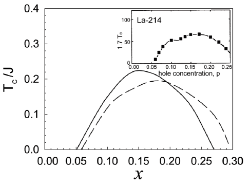
FIG. 2.: The superconducting transition temperature as a function of the hole doping concentration in the d-wave symmetry for $t/J=2.5$ and $t^{\prime}/t=0.3$ (solid line) and $t/J=2.5$ and $t^{\prime}=0$ (dashed line). Inset: the experimental result taken from Ref. [11].

Now we turn to discuss the effect of $t^{\prime}$ on the SC transition temperature. As in the case of the $t$-$J$ model [14], the SC transition temperature $T_{c}$ occurring in the case of the SC gap parameter $\Delta=0$ in Eq. (11) is identical to the dressed holon pair transition temperature occurring in the case of the effective holon pairing gap parameter $\bar{\Delta}_{hZ}=0$. In this case, we have performed a calculation for the doping dependence of the SC transition temperature, and the result of $T_{c}$ as a function of the hole doping concentration in the d-wave symmetry for $t/J=2.5$ and $t^{\prime}/J=0.3$ (solid line) and $t/J=2.5$ and $t^{\prime}=0$ (dashed line) is plotted in Fig. 2 in comparison with the experimental result [11] (inset). Our result shows that the maximal SC transition temperature T_c of the $t$-$t^{\prime}$-$J$ model occurs around the optimal doping $x_{{\rm opt}}\approx 0.15$, and then decreases in both underdoped and overdoped regimes. Furthermore, T_c in the underdoped regime is proportional to the hole doping concentration $x$, and therefore T_c in the underdoped regime is set by the hole doping concentration [26]. This reflects that the density of the dressed holons directly determines the superfluid density in the underdoped regime. Using an reasonably estimative value of $J\sim 800$K to 1200K in doped cuprates, the SC transition temperature in the optimal doping is T${}_{c}\approx 0.22J\approx 176{\rm K}\sim 264{\rm K}$, in qualitative agreement with the experimental data [11]. In comparison with the result of the $t$-$J$ model [15], our present result also shows that $t^{\prime}$ plays an important role in enhancing the SC transition temperature of the $t$-$J$ model and in shifting the maximal value of $T_{c}$ towards to the low doping regime.

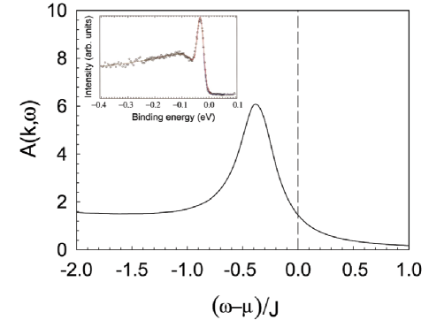
FIG. 3.: The electron spectral function with the d-wave symmetry at $[\pi,0]$ point in $x_{{\rm opt}}=0.15$ and $T=0.002J$ for $t/J=2.5$ and $t^{\prime}/J=0.3$. Inset: the experimental result taken from Ref. [29].

For cuprate superconductors, ARPES experiments have produced some interesting data that introduce important constraints on the SC theory [27]. Since cuprates superconductors are highly anisotropic materials, therefore the electron spectral function $A({\bf k},\omega)$ is dependent on the in-plane momentum [27]. Although the electron spectral function in doped cuprates obtained from ARPES is very broad in the normal-state, indicating that there are no quasiparticles [27]. However, in the SC-state, the full energy dispersion of quasiparticles has been observed [9]. According to a comparison of the density of states as measured by scanning tunnelling microscopy [28] and ARPES spectral function [29, 27] at $[\pi,0]$ point on identical samples, it has been shown that the most contributions of the electron spectral function come from $[\pi,0]$ point. In addition, the d-wave gap, and therefore the electron pairing energy scale, is maximized at $[\pi,0]$ point. Although the sharp SC quasiparticle peak at $[\pi,0]$ point in cuprate superconductors has been widely studied, the orgin and its implications are still under debate [9]. As a test of the kinetic energy driven superconductivity in doped cuprates [14], we now study this issue. For discussions of the electron spectral function, we need to calculate the electron diagonal Green’s function $G(i-j,t-t^{\prime})=\langle\langle C_{i\sigma}(t);C^{\dagger}_{j\sigma}(t^{\prime})\rangle\rangle$, which is a convolution of the dressed spin Green’s function and dressed holon diagonal Green’s function, and can be evaluated in terms of the MF dressed spin Green’s function $D^{(0)}(p)$ and dressed holon diagonal Green’s function $g(k)$ in Eq. (7a) as,

$$G({\bf k},\omega) = {1\over N}\sum_{{\bf p}}Z_{F}{B_{{\bf p}}\over 2\omega_{{\bf p}}}\left\{\left({U^{2}_{h{\bf p+k}}\over\omega+E_{h{\bf p+k}}-\omega_{{\bf p}}}\right.\right.$$ (38)

$$+ \left.{V^{2}_{h{\bf p+k}}\over\omega-E_{h{\bf p+k}}+\omega_{{\bf p}}}\right)[n_{F}(E_{h{\bf p+k}})+n_{B}(\omega_{{\bf p}})]$$ (39)

$$+ [1-n_{F}(E_{h{\bf p+k}})+n_{B}(\omega_{{\bf p}})]$$ (40)

$$\times \left.\left({U^{2}_{h{\bf p+k}}\over\omega+E_{h{\bf p+k}}+\omega_{{\bf p}}}+{V^{2}_{h{\bf p+k}}\over\omega-E_{h{\bf p+k}}-\omega_{{\bf p}}}\right)\right\},$$ (41)

then from this electron diagonal Green’s function, the electron spectral function $A({\bf k},\omega)=-2{\rm Im}G({\bf k},\omega)$ is obtained as,

$$A({\bf k},\omega) = {1\over N}\sum_{{\bf p}}Z_{F}{B_{{\bf p}}\over 2\omega_{{\bf p}}}\left\{[n_{F}(E_{h{\bf p+k}})+n_{B}(\omega_{{\bf p}})]\right.$$ (42)

$$\times [U^{2}_{h{\bf p+k}}\delta(\omega+E_{h{\bf p+k}}-\omega_{{\bf p}})$$ (43)

$$+ V^{2}_{h{\bf p+k}}\delta(\omega-E_{h{\bf p+k}}+\omega_{{\bf p}})]$$ (44)

$$+ [1-n_{F}(E_{h{\bf p+k}})+n_{B}(\omega_{{\bf p}})]$$ (45)

$$\times [U^{2}_{h{\bf p+k}}\delta(\omega+E_{h{\bf p+k}}+\omega_{{\bf p}})$$ (46)

$$+ \left.V^{2}_{h{\bf p+k}}\delta(\omega-E_{h{\bf p+k}}-\omega_{{\bf p}})]\right\}.$$ (47)

We have performed the calculation for this electron spectral function, and the result of $A({\bf k},\omega)$ at $[\pi,0]$ point in the optimal doping $x_{{\rm opt}}=0.15$ with $T=0.002J$ for $t/J=2.5$ and $t^{\prime}/J=0.3$ is plotted in Fig. 3 in comparison with the experimental result [29] (inset). Our result shows that there is a sharp SC quasiparticle peak near the electron Fermi surface at $[\pi,0]$ point, and the position of this SC quasiparticle peak is located at $\omega_{{\rm peak}}\approx 0.4J\approx 0.028$eV$\sim 0.04$eV, which is quantitatively consistent with the $\omega_{{\rm peak}}\approx 0.03$eV observed [29] in the cuprate superconductor Bi₂Sr₂CaCu₂O_8+x. Our result also shows that the dressed holon pairs condense with the d-wave symmetry in a wide range of the doping concentration, then the electron Cooper pairs originating from the dressed holon pairing state are due to the charge-spin recombination, and their condensation automatically gives the electron quasiparticle character. Furthermore, we have discussed the temperature dependence of the electron spectral function and overall quasiparticle dispersion, and these and related theoretical results will be presented elsewhere.

Our present result also indicates that the SC-state of cuprate superconductors is the conventional BCS like [3], this can be understood from the electron diagonal and off-diagonal Green’s functions in Eqs. (12) and (10), which can be rewritten as,

$$G({\bf k},\omega) = {1\over N}\sum_{{\bf p}}Z_{F}{B_{{\bf p}}\over 4\omega_{{\bf p}}}\left\{\left({U^{2}_{h{\bf p+k}}\over\omega+E_{h{\bf p+k}}-\omega_{{\bf p}}}\right.\right.$$ (49)

$$+ {U^{2}_{h{\bf p+k}}\over\omega+E_{h{\bf p+k}}+\omega_{{\bf p}}}+{V^{2}_{h{\bf p+k}}\over\omega-E_{h{\bf p+k}}+\omega_{{\bf p}}}$$ (50)

$$+ \left.{V^{2}_{h{\bf p+k}}\over\omega-E_{h{\bf p+k}}-\omega_{{\bf p}}}\right){\rm coth}[{1\over 2}\beta\omega_{{\bf p}}]$$ (51)

$$+ {\rm tanh}[{1\over 2}\beta E_{h{\bf p+k}}]\left({U^{2}_{h{\bf p+k}}\over\omega+E_{h{\bf p+k}}+\omega_{{\bf p}}}\right.$$ (52)

$$- {U^{2}_{h{\bf p+k}}\over\omega+E_{h{\bf p+k}}-\omega_{{\bf p}}}+{V^{2}_{h{\bf p+k}}\over\omega-E_{h{\bf p+k}}-\omega_{{\bf p}}}$$ (53)

$$- \left.\left.{V^{2}_{h{\bf p+k}}\over\omega-E_{h{\bf p+k}}+\omega_{{\bf p}}}\right)\right\},$$ (54)

$$\Gamma^{\dagger}({\bf k},\omega) = {1\over N}\sum_{{\bf p}}Z_{F}{\bar{\Delta}_{hZ}({\bf p+k})\over 2E_{h{\bf p+k}}}{B_{{\bf p}}\over 4\omega_{{\bf p}}}\left\{{\rm coth}[{1\over 2}\beta\omega_{{\bf p}}]\right.$$ (55)

$$\times \left({1\over\omega-E_{h{\bf p+k}}-\omega_{{\bf p}}}+{1\over\omega-E_{h{\bf p+k}}+\omega_{{\bf p}}}\right.$$ (56)

$$- \left.{1\over\omega+E_{h{\bf p+k}}+\omega_{{\bf p}}}-{1\over\omega+E_{h{\bf p+k}}-\omega_{{\bf p}}}\right)$$ (57)

$$+ {\rm tanh}[{1\over 2}\beta E_{h{\bf p+k}}]\left({1\over\omega-E_{h{\bf p+k}}-\omega_{{\bf p}}}\right.$$ (58)

$$- {1\over\omega-E_{h{\bf p+k}}+\omega_{{\bf p}}}-{1\over\omega+E_{h{\bf p+k}}+\omega_{{\bf p}}}$$ (59)

$$+ \left.\left.{1\over\omega+E_{h{\bf p+k}}-\omega_{{\bf p}}}\right)\right\},$$ (60)

respectively. Since the dressed spins center around $[\pm\pi,\pm\pi]$ in the Brillouin zone in the mean-field level [13, 14, 15], therefore the above electron diagonal and off-diagonal Green’s functions can be approximately reduced in terms of $\omega_{{\bf p}=\pm\pi,\pm\pi}\sim 0$ and the equation [13, 14] $1/2=\langle S_{i}^{z}S_{i}^{z}\rangle=1/N\sum_{{\bf p}}B_{{\bf p}}{\rm coth}(\beta\omega_{{\bf p}}/2)/(2\omega_{{\bf p}})$ as,

$$g({\bf k},\omega) \propto Z_{F}{V^{2}_{{\bf k}}\over\omega-E_{{\bf k}}}+Z_{F}{U^{2}_{{\bf k}}\over\omega+E_{{\bf k}}},$$ (62)

$$\Gamma^{\dagger}({\bf k},\omega) \propto Z_{F}{\bar{\Delta}_{hZ}({\bf k})\over 2E_{{\bf k}}}\left({1\over\omega-E_{{\bf k}}}+{1\over\omega+E_{{\bf k}}}\right),$$ (63)

with the electron quasiparticle coherence factors $U^{2}_{{\bf k}}\propto V^{2}_{{\bf k+k_{A}}}$ and $V^{2}_{{\bf k}}\propto U^{2}_{{\bf k+k_{A}}}$, and electron quasiparticle spectrum $E_{{\bf k}}\propto E_{h{\bf k+k_{A}}}$, with ${\bf k_{A}}=[\pi,\pi]$, i.e., the hole-like dressed holon quasiparticle coherence factors $U_{h{\bf k}}$ and $V_{h{\bf k}}$ have been transferred into the electron quasiparticle coherence factors $U_{{\bf k}}$ and $V_{{\bf k}}$ by the convolution of the dressed spin Green’s function and dressed holon diagonal Green’s function due to the charge-spin recombination, this is why the basic BCS formalism [9] is still valid in discussions of the doping dependence of the effective SC gap parameter and SC transition temperature, and electron spectral function [9], although the pairing mechanism is driven by the kinetic energy by exchanging dressed spin excitations, and other exotic properties are beyond the BCS theory.

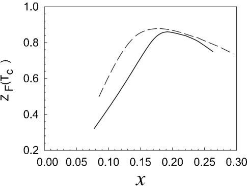
FIG. 4.: The quasiparticle coherent weight $Z_{F}(T_{c})$ as a function of the hole doping concentration for $t/J=2.5$ and $t^{\prime}/t=0.3$ (solid line) and $t/J=2.5$ and $t^{\prime}=0$ (dashed line).

The essential physics of superconductivity in the present $t$-$t^{\prime}$-$J$ model is the same as that in the $t$-$J$ model [14, 15]. The antisymmetric part of the self-energy function $\Sigma^{(h)}_{1o}({\bf k})$ (then $Z_{F}$) describes the dressed holon (then electron) quasiparticle coherence, and therefore $Z_{F}$ is closely related to the SC quasiparticle density, while the self-energy function $\Sigma^{(h)}_{2}({\bf k})$ describes the effective dressed holon (then electron) pairing gap function. In particular, both $Z_{F}$ and $\Sigma^{(h)}_{2}({\bf k})$ are doping and temperature dependent. Since the SC-order is established through an emerging quasiparticle [29, 30], therefore the SC-order is controlled by both gap function and quasiparticle coherence, and is reflected explicitly in the self-consistent equations (8a) and (8b). The dressed holons (then electrons) interact by exchanging the dressed spins and that this interaction is attractive. This attractive interaction leads to form the dressed holon pairs (then electron Cooper pairs). The perovskite parent compound of doped cuprate superconductors is a Mott insulator, when holes are doped into this insulator, there is a gain in the kinetic energy per hole proportional to $t$ due to hopping, but at the same time, the spin correlation is destroyed, costing an energy of approximately $J$ per site, therefore the doped holes into the Mott insulator can be considered as a competition between the kinetic energy ($xt$) and magnetic energy ($J$), and the magnetic energy decreases with increasing doping. In the underdoped and optimally doped regimes, the magnetic energy is rather too large, and the dressed holon (then electron) attractive interaction by exchanging the dressed spin is also rather strong to form the dressed holon pairs (then electron Cooper pairs) for the most dressed holons (then electrons), therefore the number of the dressed holon pairs (then electron Cooper pairs), SC transition temperature [26], and quasiparticle coherent weight [29, 30] are proportional to the hole doping concentration. However, in the overdoped regime, the magnetic energy is relatively small, and the dressed holon (then electron) attractive interaction by exchanging the dressed spin is also relatively weak, in this case, not all dressed holons (then electrons) can be bounden as dressed holon pairs (then electron Cooper pairs) by the weak attractive interaction, and therefore the number of the dressed holon pairs (then electron Cooper pairs), SC transition temperature [11], and quasiparticle coherent weight [30] decrease with increasing doping. To show this point clearly, we plot the quasiparticle coherent weight $Z_{F}(T_{c})$ as a function of the hole doping concentration for $t/J=2.5$ and $t^{\prime}/t=0.3$ (solid line) and $t/J=2.5$ and $t^{\prime}=0$ (dashed line) in Fig. 4. As seen from Fig. 4, the doping dependent behavior of the quasiparticle coherent weight resembles that of the superfluid density in cuprate superconductors, i.e., $Z_{F}(T_{c})$ grows linearly with the hole doping concentration in the underdoped and optimally doped regimes, and then decreases with increasing doping in the overdoped regime, which leads to that the SC transition temperature reaches a maximum in the optimal doping, and then decreases in both underdoped and overdoped regimes. The behavior of the doping dependence of $Z_{F}$ in Fig. 4 is consistent with the experimental result [29, 30], where the quasiparticle coherent weight increases monotonically with increasing doping in the underdoped and optimally doped regimes [29], and then decreases with increasing doping in the overdoped regime [30]. On the other hand, the electronic structure becomes asymmetric and hole doping shifts the Fermi surface to the van Hove singularity when the additional second neighbor hopping $t^{\prime}$ is introduced in the $t$-$J$ model [31], which leads to increase the density of states at the Fermi energy, then the SC correlation is enhanced. Furthermore, the additional second neighbor hopping $t^{\prime}$ in the $t$-$J$ model is equivalent to increase the kinetic energy. These are also why $t^{\prime}$ plays an important role in enhancing the SC transition temperature of the $t$-$J$ model under the kinetic energy driven SC mechanism.

In summary, we have discussed the effect of the additional second neighbor hopping $t^{\prime}$ on the SC-state of the $t$-$J$ model based on the kinetic energy driven SC mechanism. Our result shows that $t^{\prime}$ plays an important role in enhancing the SC transition temperature of the $t$-$J$ model. Within the $t$-$t^{\prime}$-$J$ model, we show that the SC-state of cuprate superconductors is the conventional BCS like, so that the basic BCS formalism is still valid in quantitatively reproducing the doping dependence of the effective SC gap parameter and SC transition temperature, and electron spectral function, although the pairing mechanism is driven by the kinetic energy by exchanging dressed spin excitations, and other exotic magnetic properties are beyond the BCS theory.

Superconductivity in cuprates emerges when charge carriers, holes or electrons, are doped into Mott insulators [1, 32]. Both hole-doped and electron-doped cuprate superconductors have the layered structure of the square lattice of the CuO₂ plane separated by insulating layers [1, 32]. In particular, the symmetry of the SC order parameter is common in both case [2, 33], manifesting that two systems have similar underlying SC mechanism. On the other hand, the strong electron correlation is common for both hole-doped and electron-doped cuprates, then it is possible that superconductivity in electron-doped cuprates is also driven by the kinetic energy as in hole-doped case. Within the $t$-$t^{\prime}$-$J$ model, we [34] have discussed this issue, and found that in analogy to the phase diagram of the hole-doped case, superconductivity appears over a narrow range of the electron doping concentration in the electron-doped side, and the maximum achievable SC transition temperature in the optimal doping in the electron-doped case is much lower than that of the hole-doped side due to the electron-hole asymmetry.

REFERENCES

[1] See, e.g., M.A. Kastner et al., Rev. Mod. Phys.
70, 897 (1998).
[2] See, e.g., C.C. Tsuei and J.R. Kirtley, Rev.
Mod. Phys. 72, 969 (2000).
[3] J. Bardeen, L.N. Cooper, and J.R. Schrieffer,
Phys. Rev. 108, 1175 (1957).
[6] H.J.A. Molegraaf et al., Science 295,
2239 (2002).
[7] K. Yamada et al., Phys. Rev. B57, 6165
(1998); P. Dai et al., Phys. Rev. B63, 54525 (2001); N.B.
Christensen et al., cond-mat/0403439.
[8] S. Wakimoto et al., Phys. Rev. Lett. 92,
217004 (2004); M. Fujita et al., Phys. Rev. B65, 064505
(2002); S. Wakimoto et al., Phys. Rev. B60, R769 (1999).
[9] H. Matsui et al., Phys. Rev. Lett. 90,
217002 (2003).
[10] P.W. Anderson, Science 235, 1196
(1987).
[11] See, e.g., J.L. Tallon et al., Phys. Rev.
B68, 180501
(2003).
[12] R.B Laughlin, Phys. Rev. Lett. 79,
1726 (1997); J. Low. Tem. Phys. 99, 443 (1995).
[13] Shiping Feng et al., J. Phys. Condens. Matter
16, 343 (2004); Shiping Feng et al., Mod. Phys. Lett. B17, 361 (2003); Shiping Feng et al., Phys. Rev. B49, 2368
(1994).
[14] Shiping Feng, Phys. Rev. B68, 184501
(2003).
[15] Tianxing Ma, Huaiming Guo, and Shiping Feng,
Mod. Phys. Lett. B18, 895 (2004); Shiping Feng and Tianxing
Ma, cond-mat/0407310.
[16] B.O. Well et al., Phys. Rev. Lett. 74, 964
(1995); C. King et al., Phys. Rev. Lett. 80, 4245 (1998).
[17] K. Tanaka et al., Phys. Rev. B 70,
092503 (2004).
[18] Z.-X. Shen et al., Phys. Rev. Lett. 70,
1553 (1993); H. Ding et al., Phys. Rev. B54, R9678 (1996).
[22] P. Chaudhari, and S.Y. Lin, Phys. Rev. Lett.
72, 1084 (1994); D.H. Wu et al., Phys. Rev. Lett. 70,
85 (1993); S.M. Anlage et al., Phys. Rev. B44, 9764 (1991).
[23] J.A. Martindale et al., Phys. Rev. B47,
9155 (1993); W.N. Hardy et al., Phys. Rev. Lett. 70, 3999
(1994); D.A. Wollman et al., Phys. Rev. Lett. 71, 2134
(1993).
[24] H.H. Wen et al., Europhys. Lett. 64, 790
(2003).
[25] C.T. Shih et al., Phys. Rev. Lett. 92,
227002 (2004).
[26] Y.J. Uemura et al., Phys. Rev. Lett. 62,
2317 (1989); Y.J. Uemura et al., Phys. Rev. Lett. 66, 2665
(1991).
[27] See, e.g., A. Damascelli, Z. Hussain, and Z.-X.
Shen, Rev. Mod. Phys. 75, 475 (2003).
[28] Y. DeWilde et al., Phys. Rev. Lett. 80, 153 (1998).
[29] H. Ding et al., Phys. Rev. Lett. 87,
227001 (2001).
[30] R.H. He et al., Phys. Rev. B69, 220502
(2004).
[31] D.M. Newns et al., Phys. Rev. B43,
3075 (1991).
[32] Y. Tokura, H. Takagi, and S. Uchida, Nature
337, 345 (1989).
[33] C.C. Tsuei and J.R. Kirtley, Phys. Rev. Lett.
85, 182 (2000).
[34] Tianxing Ma and Shiping Feng, Phys. Lett. A
339, 131 (2005).