On Defect-Mediated Transitions in Bosonic Planar Lattices

Abstract

We discuss the finite-temperature properties of Bose-Einstein condensates loaded on a $2D$ optical lattice. In an experimentally attainable range of parameters the system is described by the $XY$ model, which undergoes a Berezinskii-Kosterlitz-Thouless (BKT) transition driven by the vortex pair unbinding. The interference pattern of the expanding condensates provides the experimental signature of the BKT transition: near the critical temperature, the $\vec{k}=0$ component of the momentum distribution sharply decreases.

Bose-Einstein condensates (BECs) are nowadays routinely stored in $1D$ [1, 2, 3, 4, 5], $2D$ [6] and $3D$ [7] optical lattices. In this paper we review and further discuss the finite-temperature properties of Bose-Einstein condensates loaded on a $2D$ optical lattice [8]: there we showed that at a critical temperature lower than the temperature $T_{BEC}$ at which condensation in each well occurs, $2D$ lattices of BECs may undergo a phase transition to a superfluid regime where the phases of the single-well condensates are coherently aligned allowing for the observation of a Berezinskii-Kosterlitz-Thouless (BKT) transition.

The BKT transition is the paradigmatic example of a defect-mediated transition [9] which is exhibited by the two-dimensional $XY$ model [10, 11], describing $2$-components spins on a two-dimensional lattice. In the low-temperature phase, characterized by the presence of bound vortex-antivortex pairs, the spatial correlations exhibit a power-law decay; above a critical temperature $T_{BKT}$, the decay is exponential and there is a proliferation of free vortices. The BKT transition has been observed in superconducting Josephson arrays [12] and its predictions are well verified in the measurements of the superfluid density in ${}^{4}He$ films [13]. In finite magnetic systems with planar symmetry [14], the BKT transition point is signaled by the drop of a suitably defined magnetization [15]. We shall discuss in the sequel the analogous of this magnetization for atomic systems.

For $2D$ optical lattices, when the polarization vectors of the two standing wave laser fields are orthogonal, the resulting periodic potential for the atoms is $V_{opt}=V_{0}[\sin^{2}{(kx)}+\sin^{2}{(ky)}]$ where $k=2\pi/\lambda$ is the wavevector of the laser beams. The potential maximum of a single standing wave $V_{0}=sE_{R}$ may be controlled by changing the intensity of the optical lattice beams, and it is conveniently measured in units of the recoil energy $E_{R}=\hbar^{2}k^{2}/2m$ ($m$ is the atomic mass), while, typically, $s$ can vary from $0$ up to $30$. Gravity is assumed to act along the $z$-axis. Usually, superimposed to the optical potential there is an harmonic magnetic potential $V_{m}=(m/2)[\omega_{r}^{2}(x^{2}+y^{2})+\omega_{z}^{2}z^{2}]$, where $\omega_{z}$ ($\omega_{r}$) is the axial (radial) trapping frequency. The minima of the lattice are located at the points $\vec{j}=(j_{1},j_{2})\cdot\frac{\lambda}{2}$ with $j_{1}$ and $j_{2}$ integers, and the potential around the minima is $V_{opt}\approx\frac{m}{2}\tilde{\omega}_{r}^{2}[(x-\lambda j_{1}/2)^{2}+(y-\lambda j_{2}/2)^{2}]$ with $\tilde{\omega}_{r}=\sqrt{2V_{0}k^{2}/m}$. When $\tilde{\omega}_{r}\gg\omega_{r},\omega_{z}$, the system realizes a square array of tubes, i.e. an array of harmonic traps elongated along the $z$-axis [6]. In the following we analyze only the situation in which the axial degrees of freedom are frozen out, which is realizable if $\omega_{z}$ is sufficiently large. We also assume that the harmonic oscillator length of the magnetic potential $\sqrt{\hbar/m\omega_{r}}$ is enough larger than the size $L$ (in lattice units) of the optical lattice in order to reduce density inhomogeneity effects and to allow for a safe control of finite size effects.

When all the relevant energy scales are small compared to the excitation energies one can expand the field operator [16] as $\hat{\Psi}(\vec{r},t)=\sum_{\vec{j}}\hat{\psi}_{\vec{j}}(t)\Phi_{\vec{j}}(\vec{r})$ with $\Phi_{\vec{j}}(\vec{r})$ the Wannier wavefunction localized in the $\vec{j}$-th well (normalized to $1$) and $\hat{N}_{\vec{j}}=\hat{\psi}^{{\dagger}}_{\vec{j}}\hat{\psi}_{\vec{j}}$ the bosonic number operator. Substituting the expansion in the full quantum Hamiltonian describing the bosonic system, leads to the Bose-Hubbard model (BHM) [17, 16]

$$\hat{H}=-K\sum_{<\vec{i},\vec{j}>}(\hat{\psi}^{{\dagger}}_{\vec{i}}\hat{\psi}_{\vec{j}}+h.c.)+\sum_{\vec{j}}\Bigg{[}{U\over 2}\hat{N}_{\vec{j}}(\hat{N}_{\vec{j}}-1)\Bigg{]}$$ (1)

where $\sum_{<\vec{i},\vec{j}>}$ denotes a sum over nearest neighbours, $U=(4\pi\hbar^{2}a/m)\int d\vec{r}\,\Phi_{\vec{j}}^{4}$ ($a$ is the $s$-wave scattering length) and $K\simeq-\int d\vec{r}\,\big{[}\frac{\hbar^{2}}{2m}\vec{\nabla}\Phi_{\vec{i}}\cdot\vec{\nabla}\Phi_{{\vec{j}}}+\Phi_{\vec{i}}V_{ext}\Phi_{\vec{j}}\big{]}$.

Upon defining $J\approx 2KN_{0}$ (where $N_{0}$ is the average number of atoms per site), when $N_{0}\gg 1$ and $J/N_{0}^{2}\ll U$, the BHM reduces to $\hat{H}=H_{XY}-{U\over 2}\sum_{\vec{j}}\frac{\partial^{2}}{\partial\theta_{\vec{j}}^{2}}$, which describes the so-called quantum phase model (see e.g. [18, 19]): $\theta_{\vec{j}}$ is the phase of the $j$-th condensate and

$$H_{XY}=-J\sum_{<\vec{i},\vec{j}>}\cos{(\theta_{\vec{i}}-\theta_{\vec{j}})}$$ (2)

stands for the Hamiltonian of the classical $XY$ model. When $J\gg U$ and at temperatures $T\gg U/k_{B}$, the quantum phase Hamiltonian may be well approximated by Eq.(2); therefore, the pertinent partition function describing the thermodynamic behaviour of the BECs stored in an optical lattice can be computed in these limits with the classical $XY$ model.

We remark that the BHM - for $U=0$ - describes harmonic oscillators and thus cannot sustain any BKT transition. However, in the limits above specified ($N_{0}\gg 1$ and $J/N_{0}^{2}\ll U\ll J$) the Bose-Hubbard Hamiltonian reduces in the $XY$ model (2), which displays the BKT transition. We observe that in the chosen range of parameters, the condition $UN_{0}^{2}/J=UN_{0}/2K\gg 1$, satisfies the finite-temperature stability criterion recently derived in [20]. In superconducting networks $N_{0}$ is the average number of excess Cooper pairs and thus, the requirements $N_{0}\gg 1$ and $J/N_{0}^{2}\ll U$ are always satisfied; at variance, in bosonic lattices $N_{0}$ varies usually between $\sim 1$ and $\sim 10^{3}$ and the validity of the mapping in the quantum phase Hamiltonian is not always guaranteed.

A simple estimate of the coefficients $J$ and $U$ may be obtained by approximating the Wannier functions with gaussians, whose widths are determined variationally [8]. For a $2D$ lattice with $V_{0}$ between $20$ and $25E_{R}$ (and $N_{0}\approx 170$ as in [6]), the conditions $J\gg U\gg J/N_{0}^{2}$ are rather well satisfied and the BKT critical temperature, $T_{BKT}\sim J/k_{B}$, is between $10$ and $30nK$.

We observe that, using a coarse-graining approach to determine the finite-temperature phase-boundary line of the Bose-Hubbard model (1) [21], one gets - in $2D$ for $N_{0}\gg 1$ and $J/U\gg 1$ - a critical temperature $T_{BKT}\approx J/k_{B}$. Indeed, within a coarse-graining approach, the phase-boundary line of the Bose-Hubbard model at a temperature $T$ is given by [21]

$$1=Kd\int_{0}^{\beta}d\tau G(\tau)$$ (3)

where $d$ is the lattice dimension and $\beta=1/k_{B}T$. In Eq.(3) $G(\tau)$ is the correlation function, which, for $N_{0}\gg 1$, is given by

$$G(\tau)\approx N_{0}\frac{\vartheta_{3}\bigg{(}\pi(N_{0}+\tau/\beta),q\bigg{)}}{\vartheta_{3}\bigg{(}\pi N_{0},q\bigg{)}}e^{-\tau U(1-\tau/\beta)/2}$$ (4)

with $\vartheta_{3}(z,q)=1+2\sum_{n=1}^{\infty}\cos{(2nz)}\cdot q^{n^{2}}$. Since $d=2$, and $J=2KN_{0}$, from Eq.(3) it follows $1=JG(\omega=0)/N_{0}$ where $G(\omega=0)=\int_{0}^{\beta}d\tau G(\tau)$; one has then

$$\frac{G(\omega=0)}{N_{0}}=\frac{\sum_{m}\exp{(-\beta U\phi_{n}^{2}/2)}\cdot\frac{1-\exp{(-\beta U(\phi_{n}+1/2)}}{U(\phi_{m}+1/2)}}{\sum_{m}\exp{(-\beta U\phi_{n}^{2}/2)}}:$$ (5)

where $\phi_{m}=N_{0}-m$. Eq.(5) yields, for $U\ll k_{B}T$, $G(\omega=0)/N_{0}\approx\beta$, thus implying $\beta J\approx 1$, i.e. $k_{B}T_{BKT}\approx J$, in fair agreement with $XY$ estimates.

We notice that the $XY$ Hamiltonian, in the limits $N_{0}\gg 1$ and $J\gg U\gg J/N_{0}^{2}$, can be retrieved extending the Gross-Pitaevskii (GP) Hamiltonian to finite temperature $T\gg U/k_{B}$. In fact, replacing the tight-binding ansatz $\Psi(\vec{r},t)=\sum_{\vec{j}}\psi_{\vec{j}}(t)\Phi_{\vec{j}}(\vec{r})$ (where $\psi_{\vec{j}}$ are classical fields and not operators) in the GP Hamiltonian one gets the lattice Hamiltonian $H=-K\sum_{<\vec{i},\vec{j}>}(\psi^{\ast}_{\vec{i}}\psi_{\vec{j}}+c.c.)+(U/2)\sum_{\vec{j}}N_{\vec{j}}(N_{\vec{j}}-1)$, which is the classical version of the Bose-Hubbard model ($N_{\vec{j}}\equiv\mid\psi_{\vec{j}}\mid^{2}$). Writing $N_{\vec{j}}=N_{0}+\delta N_{\vec{j}}$, one may neglect the quadratic terms [i.e. $(\delta N_{\vec{j}})^{2}$] in the hopping part of the Hamiltonian $-K\sum_{<\vec{i},\vec{j}>}(\psi^{\ast}_{\vec{i}}\psi_{\vec{j}}+c.c.)$, which then reduces to $H_{XY}$ (2).

Accurate Monte Carlo simulations yield - for the $XY$ model - the BKT critical temperature $T_{BKT}=0.898J/k_{B}$ [22]. When $U\ll J$, a BKT transition still occurs at a slightly lower critical temperature $T_{BKT}(U)$. To evaluate more accurately the effects of the interaction term on the BKT critical temperature one may use a semiclassical approximation to evaluate a renormalized Josephson energy [23, 24]: the renormalization group equations yields then the following equation for ${\cal K}\equiv\beta T_{BKT}(U)$

$$2-\pi{\cal K}\Bigr{[}1-\frac{1}{4{\cal K}}-\frac{1}{X_{u}{\cal K}^{3}}\,g({\cal K},X_{u})\Bigr{]}=0$$ (6)

where $X_{u}=U/\pi J$ and $g({\cal K},X_{u})\equiv\sum_{n=1}^{\infty}[X_{u}{\cal K}^{2}/2-(n^{2}/2)ln(1+X_{u}{\cal K}^{2}/n^{2})]$. One may see [25] that for $U/J<36/\pi$, Eq.(6) has an unique solution; at variance, for $U/J>36/\pi$ Eq.(6) does not have any solution. The value $U/J=36/\pi$ is in reasonable agreement with the known mean-field prediction $2zJ/U\approx 1$ for the $T=0$ phase transition (see, e.g., Eq. (30) of Ref. [26] for $N_{0}\gg 1$). In the inset of Fig.1 we plot the value of $T_{BKT}(U)/T_{BKT}$ (where $T_{BKT}$ is the BKT critical temperature of the XY model with $U=0$) as a function of $U/J$ from the numerical solution of Eq.(6).

The emerging physical picture is the following: There are two relevant temperatures for the system, the temperature $T_{BEC}$, at which in each well there is a condensate, and the temperature $T_{BKT}$ at which the condensates phases start to coherently point in the same direction. Of course, in order to have well defined condensates phases one should have $T_{BKT}<T_{BEC}$. The critical temperature $T_{BEC}\approx 0.94\hbar N_{0}^{1/3}\bar{\omega}/k_{B}$ where $\bar{\omega}=(\tilde{\omega}_{r}^{2}\omega_{z})^{1/3}$. With the numerical values given in [6], $T_{BEC}$ turns out to be $\gtrsim\ 500nK$ for $s\gtrsim 20$. When $T<T_{BEC}$, the atoms in the well $\vec{j}$ of the $2D$ optical lattice may be described by a macroscopic wavefunction $\psi_{\vec{j}}$. Furthermore, when the fluctuations around the average number of atoms per site $N_{0}\gg 1$ are strongly suppressed, one may put, apart from the factor $\sqrt{N_{0}}$ constant across the array, $\psi_{\vec{j}}=e^{i\theta_{\vec{j}}}$. The temperature $T_{BKT}$ is of order of $J/k_{B}$: with the experimental parameters of [6] and $V_{0}$ between $20$ and $25E_{R}$, one has that $T_{BKT}$ is between $10$ and $30nK$, which is sensibly smaller than the condensation temperature $T_{BEC}$ of the single well. A similar picture describes also $2D$ arrays of superconducting Josephson junctions [18, 19]: they exhibit a temperature $T_{BCS}$ at which the metallic grains placed on the sites of the array become (separately) superconducting and the Cooper pairs may be described by macroscopic wavefunctions. At a temperature $T_{BKT}<T_{BCS}$, the array undergo a BKT transition and the system - as a whole - becomes superconducting.

The experimental signature of the BKT transition in bosonic planar lattices is obtained by measuring, as a function of the temperature, the central peak of the interference pattern obtained after turning off the confining potentials [8]. In fact, the peak of the momentum distribution at $\vec{k}=0$ is the direct analog of the magnetization of a finite size $2D$ $XY$ magnet. For the $XY$ magnets, the spins can be written as $\vec{S}_{\vec{j}}=(\cos{\theta_{\vec{j}}},\sin{\theta_{\vec{j}}})$ and the magnetization is defined as $M=(1/N)\cdot\langle\,\mid\sum_{\vec{j}}\vec{S}_{\vec{j}}\mid\,\rangle$ where $\langle\cdots\rangle$ stands for the thermal average. A spin-wave analysis at low temperatures yields $M=(2N)^{-k_{B}T/8\pi J}$ [14, 15]. With discrete BECs at $T=0$, all the phases $\theta_{\vec{j}}$ are equal at the equilibrium and the lattice Fourier transform of $\psi_{j}$, $\tilde{\psi}_{\vec{k}}=\frac{1}{N}\sum_{\vec{j}}\psi_{\vec{j}}\,\,\,e^{-i\vec{k}\cdot{\vec{j}}}$, exhibits a peak at $\vec{k}=0$ ($\vec{k}$ is in the first Brillouin zone of the $2D$ square lattice) and the magnetization is:

$$M=\langle\,\mid\tilde{\psi}_{0}\mid\,\rangle.$$ (7)

The intuitive picture of the BKT transition is then the following: at $T=0$, all the spins point in the same direction. Increasing the temperature, bound vortex pairs are thermally induced. In Fig.2, left inset, a single free vortex is depicted: we plot a configuration of the phases such that $\theta_{\vec{j}}$ equals the polar angle of the site $\vec{j}$ with respect to the core vortex (notice that with $\theta_{\vec{j}}$ equals the polar angle plus $\pi/2$ one would have the usual plot of a vortex). As one can see, a single vortex modifies the phase distribution also much far from its core and the square modulus of its lattice Fourier transform $\mid\tilde{\psi}_{\vec{k}}\mid^{2}$ has a minimum at $\vec{k}=0$. At variance, a vortex-antivortex pair [see Fig.2, right inset] modifies the phase distribution only near the center of the pair (in this sense is a defect) and its lattice Fourier transform has a maximum at $\vec{k}=0$. Increasing the temperature, vortices are thermally induced. For $T<T_{BKT}$ only bound vortex pairs are present, and in average the spins continue to point in the same direction. When the condensates expand, a large peak (i.e., a magnetization) is observed in the central $\vec{k}=0$ momentum component. Rising further the temperature, due to the increasing number of vortex pairs, the central peak density decreases from the $T=0$ value. For $T\approx T_{BKT}$ the pairs starts to unbind and free vortices begin to appear, determining a sharp decrease around $T_{BKT}$ of the magnetization. At high temperatures, only free vortices are present, leading to a randomization of the phases and to a vanishing magnetization. In Fig.1 we plot the intensity of the central peak of the momentum distribution (normalized to the value at $T=0$) in a 2D lattice as a function of the reduced temperature $k_{B}T/J$, evidencing the sharp decrease of the magnetization around the critical temperature [8].

At $t=0$ the amplitude of the $\vec{k}=0$ peak of the momentum distribution is simply given by the thermal average of $\tilde{\psi}_{0}$. By measuring the $\vec{k}=0$ peak (i.e., $\langle\,\mid\tilde{\psi}_{0}\mid^{2}\,\rangle$) at different temperatures, one obtains the results plotted in Fig.1. The figure has been obtained using a Monte Carlo simulation of the $XY$ magnet for a $40\times 40$ array: we find $k_{B}T_{C}\approx 1.07J$. In Fig.1 we also plot the low-temperature spin wave prediction [15] (solid line). At times different from $t=0$, the density profiles are well reproduced by the free expansion of the ideal gas. One obtains $\tilde{\psi}(\vec{p},t)=\chi(p_{z})e^{-i[(p_{z}+mgt)^{3}-p_{z}^{3}]/6m^{2}g\hbar}\tilde{\varphi}(p_{x},p_{y},t)$ [where $\chi(p_{x})\propto e^{-\sigma_{x}^{2}p_{x}^{2}/2\hbar^{2}}$ and similarly for $\chi(p_{y})$ and $\chi(p_{z})$], i.e. a uniformly accelerating motion along $z$ and a free motion in the plan $x-y$, with $\tilde{\varphi}(p_{x},p_{y},t)=\chi(p_{x})\chi(p_{y})\tilde{\psi}_{\vec{k}}e^{-i(p_{x}^{2}+p_{y}^{2})t/2\hbar m}$ giving the central and lateral peaks of the momentum distribution as a function of time for different temperatures.

An intense experimental work is now focusing on the Bose-Einstein condensation in two dimensions: at present a crossover to two-dimensional behaviour has been observed for $Na$ [27] and $Cs$ atoms [28]. Our analysis relies on two basic assumptions; namely, the validity of the tight-binding approximation for the Bose-Hubbard Hamiltonian and the requirement that the condensate in the optical lattice may be regarded as planar [29]. It is easy to see that the first assumption is satisfied if, at $T=0$, $V_{0}\gg\mu$ (where $\mu$ is the chemical potential), and, at finite temperature, $\hbar\tilde{\omega}_{r}\gtrsim k_{B}T$. The second assumption is much more restrictive since it requires freezing the transverse excitations; for this to happen one should require a condition on the transverse trapping frequency $\omega_{z}$. Namely, one should have that, at $T=0$, $\hbar\omega_{z}\gtrsim 8K$ and that, at finite temperature, $\hbar\omega_{z}\gtrsim k_{B}T$ (since $\omega_{z}\ll\tilde{\omega}_{r}$, the latter condition also implies that $\hbar\tilde{\omega}_{r}\gtrsim k_{B}T$). In [6] it is $V_{0}=s\cdot k_{B}\cdot 0.15\mu K$ and for $s\gtrsim 20$ the tight-binding conditions are satisfied since $10Hz\gtrsim 8K/2\pi\hbar$; furthermore, if $\omega_{z}=2\pi\cdot 1kHz$, one may safely regard our finite temperature analysis to be valid at least up to $T\sim 50nK$. We notice that the experimental signature for the BKT transition for a continuous (i.e., without optical lattice) weakly interacting 2D Bose gas [30] is also given by the central peak of the atomic density of the expanding condensates.

Our study evidences the possibility that Bose-Einstein condensates loaded on a $2D$ optical lattice may exhibit - at finite temperature - a new coherent behaviour in which all the phases of the condensates located in each well of the lattice point in the same direction. The finite temperature transition, which is due to the thermal atoms in each well, is mediated by vortex defects and may be experimentally detectable by looking at the interference patterns of the expanding condensates. Our analysis strengthens - and extends at finite temperature - the striking and deep analogy of bosonic planar systems with $2D$ Josephson junction arrays [1].

Acknowledgements This work has been supported by MIUR through grant No. 2001028294 and by the DOE.

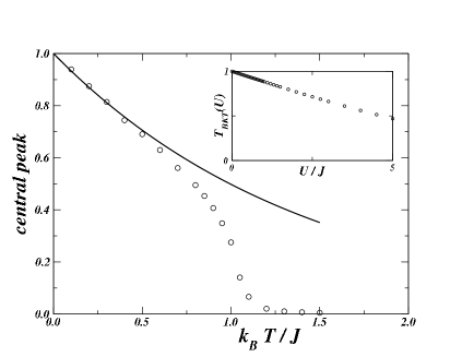
FIG. 1.: Intensity of the central peak of the momentum distribution (normalized to the value at $T=0$) as a function of the reduced temperature $t=k_{B}T/J$; empty circles: Monte Carlo simulations; solid line: low-temperature spin wave prediction [15]. Inset: the BKT critical temperature $T_{BKT}(U)$ (in units of the $XY$ critical temperature) as a function of $U/J$ from Eq.(6).

FIG. 2.: Left: a lattice vortex; right: a vortex-antivortex pair.

REFERENCES

- [1] B. P. Anderson and M. A. Kasevich, Science 282, 1686 (1998).
- [2] F. S. Cataliotti, S. Burger, C. Fort, P. Maddaloni, F. Minardi, A. Trombettoni, A. Smerzi, and M. Inguscio, Science 293, 843 (2001).
- [3] O. Morsch, J. H. Müller, M. Cristiani, D. Ciampini, and E. Arimondo Phys. Rev. Lett. 87, 140402 (2001).
- [4] W. K. Hensinger, H. Haffer, A. Browaeys, N. R. Heckenberg, K. Helmerson, C. McKenzie, G. J. Milburn, W. D. Phillips, S. L. Rolston, H. Rubinsztein-Dunlop, and B. Upcroft, Nature 412, 52 (2001).
- [5] B. Eiermann, P. Treutlein, T. Anker, M. Albiez, M. Taglieber, K.-P. Marzlin, and M. K. Oberthaler Phys. Rev. Lett. 91, 060402 (2003).
- [6] M. Greiner, I. Bloch, O. Mandel, T. W. Hänsch, and T. Esslinger, Phys. Rev. Lett. 87, 160405 (2001); Appl. Phys. B 73, 769 (2001).
- [7] M. Greiner, O. Mandel, T. Esslinger, T. W. Hänsch, and I. Bloch, Nature 415, 39 (2002).
- [8] A. Trombettoni, A. Smerzi, and P. Sodano, New J. Phys. 7, 57 (2005).
- [9] D. R. Nelson, in Phase Transitions and Critical Phenomena, vol. 7, eds. C. Domb and J. L. Lebowitz (New York, Academic Press, 1983) and references therein.
- [10] P. Minnaghen, Rev. Mod. Phys. 59, 1001 (1987).
- [11] L. P. Kadanoff, Statistical Physics: Statics, Dynamics and Renormalization, (Singapore, World Scientific, 2000), Chapt.s 16-17 and reprints therein.
- [12] D. J. Resnick, J. C. Garland, J. T. Boyd, S. Shoemaker, and R. S. Newrock, Phys. Rev. Lett. 47, 1542 (1981).
- [13] D. J. Bishop and J. D. Reppy, Phys. Rev. Lett. 40, 1727 (1978).
- [14] S. T. Bramwell and P. C. W. Holdsworth, J. Phys.: Condensed Matter 5, L53 (1993); Phys. Rev. B 49, 8811 (1994).
- [15] V.L. Berezinskii and A.Ya. Blank, Sov. Phys. JETP 37, 369 (1973).
- [16] D. Jaksch, C. Bruder, J. I. Cirac, C. W. Gardiner, and P. Zoller, Phys. Rev. Lett. 81, 3108 (1998).
- [17] M. P. A. Fisher, P. B. Weichman, G. Grinstein, and D. S. Fisher, Phys. Rev. B 40, 546 (1989).
- [18] E. Simànek, Inhomogeneous Superconductors, Oxford University Press, New York, 1994.
- [19] R. Fazio and H. van der Zant, Phys. Rep. 355, 235 (2001).
- [20] S. Tsuchiya and A. Griffin, Phys. Rev. A 70, 023611 (2004).
- [21] A. P. Kampf and G. T. Zimanyi, Phys. Rev. B 47, 279 (1993).
- [22] R. Gupta, J. DeLapp, G. G. Batrouni, G. C. Fox, C. F. Baillie, and J. Apostolakis, Phys. Rev. Lett. 61, 1996 (1988).
- [23] J.V. José, Phys. Rev. B 29, 2836 (1984).
- [24] C. Rojas and J.V. José, Phys. Rev. B 54, 12361 (1996).
- [25] A. Smerzi, P. Sodano, and A. Trombettoni, J. Phys. B 37, S265 (2004).
- [26] D. van Oosten, P. van der Straten, and H. T. C. Stoof, Phys. Rev. A 63, 053601 (2001).
- [27] A. Görlitz, J. M. Vogels, A. E. Leanhardt, C. Raman, T. L. Gustavson, J. R. Abo-Shaeer, A. P. Chikkatur, S. Gupta, S. Inouye, T. Rosenband, and W. Ketterle, Phys. Rev. Lett. 87, 130402 (2001).
- [28] M. Hammes, D. Rychtarik, B. Engeser, H.-C. Nägerl, and R. Grimm, Phys. Rev. Lett. 90, 173001 (2001).
- [29] D. S. Petrov, M. Holzmann, and G. V. Shlyapnikov, Phys. Rev. Lett. 84, 2551 (2000).
- [30] N. Prokofév, O. Ruebenacker, and B. Svistunov, Phys. Rev. Lett. 87, 270402 (2001).