Rectification in one–dimensional electronic systems

Abstract

Asymmetric current–voltage ($I(V)$) curves, known as the diode or rectification effect, in one–dimensional electronic conductors can have their origin from scattering off a single asymmetric impurity in the system. We investigate this effect in the framework of the Tomonaga–Luttinger model for electrons with spin. We show that electron interactions strongly enhance the diode effect and lead to a pronounced current rectification even if the impurity potential is weak. For strongly interacting electrons and not too small voltages, the rectification current, $I_{r}=[I(V)+I(-V)]/2$, measuring the asymmetry in the current–voltage curve, has a power–law dependence on the voltage with a negative exponent, $I_{r}\sim V^{-|z|}$, leading to a bump in the current–voltage curve.

I Introduction

Current rectification, also known as the diode effect, occurs whenever the transport characteristics in electronic conductors are asymmetric under the application of the driving voltage. This asymmetry can have various origins. Best known perhaps is the mismatch of band structures in macroscopic diodes, which leads to a potential wall that blocks the motion of the particles in one direction, while it is not seen by the particles moving in the opposite direction.

In the last years, rectification in mesoscopic and single–molecule systems has attracted much attention. Even though rectification by single asymmetric molecules has been suggested 30 years agoAviram and Ratner (1974), it has been realized experimentally in the 1990s onlyGeddes et al. (1990); Martin et al. (1993); Joachim et al. (2000). Asymmetric wave guides were constructed in the inversion layer of semiconductor heterostructuresLinke et al. (1999); Löfgren et al. (2003). Transport asymmetries have been observed in carbon nanotubesPostma et al. (2001); Papadopoulos et al. (2004) and in tunneling in quantum Hall edge statesRoddaro et al. (2003). The experimental progress has been accompanied by much theoretical activityChristen and Büttiker (1996); Reimann et al. (1997); Lehmann et al. (2002); Scheidl and Vinokur (2002); Komnik and Gogolin (2003); Sánchez and Büttiker (2004); Spivak and Zyuzin (2004); Feldman et al. (2005) with the main focus on Fermi–liquid systems.

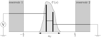
Figure 1: Sketch of system of length $L$ with a simple asymmetric potential $U(x)$, consisting in two point scatterers of different magnitude in a region $a_{U}\ll L$. The horizontal lines qualitatively represent the density profile (averaged over Friedel oscillations) expected in the system. The reservoirs determine the densities of the injected particles at the far left and right sides, and are controlled by the voltage source. The shaded area represents a more general asymmetric impurity potential, which would have a similar asymmetric density profile.

An interesting source for rectification arises when the particle interaction is strong enough that a single–particle description becomes invalid. This naturally occurs in one–dimensional systems, for which a Luttinger liquid behavior is expected. It has been known for some time nowKane and Fisher (1992) that in such systems the current is strongly affected by the presence of impurities, even when they are weak, due to their renormalization by the electron–electron interactions. One can thus expect that asymmetries in the impurity distribution leads to strongly asymmetric current–voltage curves. This issue was addressed very recently in the framework of Luttinger liquids of spinless particlesFeldman et al. (2005). The rectification current $I_{r}(V)=[I(V)+I(-V)]/2$ can be measured as the dc response to a low-frequency square voltage wave of amplitude $V$ and expresses the asymmetry of the $I-V$ curve for forward and reverse bias. It was shown that a single weak asymmetric impurity is sufficient for a pronounced rectification effect (see Fig. 1 for a sketch of the system), leading to a large rectification current, $I_{r}(V)$, at low voltages $V$. Moreover an unusual behavior of the current was revealed for systems with strong repulsive interactions: A power–law dependence of $I_{r}$ on the voltage with a negative exponent, $I_{r}\sim V^{-|z|}$, within a range $V^{*}<V<V^{**}$ [with $V^{*}$ and $V^{**}$ being expressed by some powers of the impurity potential $U$; see also below], i.e. the rectification current increases as the voltage is lowered. At $V<V^{*}$ the increase crosses over into a regular decrease such that the equilibrium condition $I=0$ at $V=0$ is met. The qualitative behavior is shown in Fig. 2.

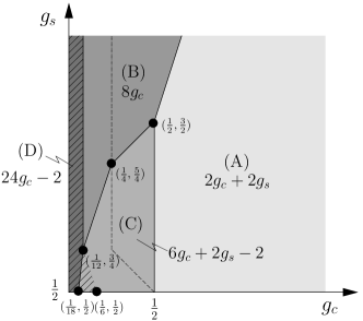
Figure 3: Diagram for the leading power–law contributions to the rectification current, $I_{r}\sim V^{z}$, for voltages $V\gtrsim V^{*}$. The exponents $z$ for the four different phases are given by the formulae in the figure (see also Table 1). The zone boundaries indicate crossover regions. On the left of the dashed line $V^{*}>0$, and on the right $V^{*}=0$ (see Eq. (11)). In the hatched area, $z<0$, and the rectification current shows the behavior sketched in Fig. 2.

In this paper we pursue this work for real electrons carrying a spin. We show that we can provide lower and upper limits for the voltage $V$, within which perturbation theory can be applied and determine the leading power–law behavior of the rectification current, $I_{r}\sim V^{z}$, as a function of the charge and spin interaction strengths, $g_{c}$ and $g_{s}$. This leads to a phase diagram for the leading power–law dependence of $I_{r}$ with a much richer structure than in the spinless case (Fig. 3). We show that, similar to the spinless case, a negative exponent $z$, $I_{r}\sim V^{-|z|}$, appears for strong repulsive electron–electron interactions within a voltage range that is determined by the bare impurity scattering strength. Fig. 3 shows our main result, the leading power–law behavior of the rectification current $I_{r}$. The hatched region in the figure marks the range of $(g_{c},g_{s})$, in which the exponent $z$ becomes negative and in which the rectification current shows the behavior sketched in Fig. 2.

The paper is organized as follows: In the next section, we introduce the model of electrons in a one–dimensional system, and argue how scattering on a single impurity can lead to rectification. We then quantitatively address this problem within the bosonization approach, and show that the most relevant power–law behavior of the rectification current can be obtained within second and third order perturbation theory. The results are listed in Table 1 and in Fig. 3. In the appendix we show that higher order perturbative contributions cannot exceed the leading second and third order expressions.

II Model and Origin of Rectification

Let us consider a one–dimensional conductor of length $L$ with electron–electron interactions that are effectively short–ranged due to screening by gates. Such a system allows a description by the Tomonaga–Luttinger model, given by the Hamiltonian

$$H =\int\mathrm{d}x\sum_{\sigma}\Bigl{\{}-\hbar v_{F}\Bigl{[}\psi_{R\sigma}^{\dagger}(x)i\partial_{x}\psi_{R\sigma}(x)-\psi_{L\sigma}^{\dagger}(x)i\partial_{x}\psi_{L\sigma}(x)\Bigr{]}$$

$$\qquad\qquad\qquad\qquad+U(x)\psi_{\sigma}^{\dagger}(x)\psi_{\sigma}(x)\Bigr{\}}$$

$$+\int\mathrm{d}x\mathrm{d}y\sum_{\sigma\sigma^{\prime}}K_{\sigma\sigma^{\prime}}(x-y)\psi_{\sigma}^{\dagger}(x)\psi_{\sigma^{\prime}}^{\dagger}(y)\psi_{\sigma^{\prime}}(y)\psi_{\sigma}(x),$$ (1)

where $\psi_{R\sigma}$ and $\psi_{L\sigma}$ are the operators for right– and left–moving electrons with spin $\sigma=\uparrow,\downarrow$, and $\psi_{\sigma}=\psi_{R\sigma}+\psi_{L\sigma}$ is the conventional electron operator. $U_{\sigma}(x)$ is the asymmetric potential (i.e. $U(x)\neq U(-x)$) localized in a small region about $x=0$. $K(x-y)$ describes the electron–electron interaction. For the following discussion it is important to assume that the long–ranged Coulomb interaction is screened by the gates, so that $K(x-y)$ becomes a short–ranged, rapidly decreasing function of $(x-y)$.

On its two ends, at $x=\pm L/2$, the system is adiabatically coupled to electrodes that serve as reservoirs of particles, and whose chemical potentials $\mu_{1,2}$ are controlled experimentally: We assume that one electrode is fixed at the ground, $\mu_{2}=\mu$, while the other one is connected to the voltage source, $\mu_{1}=\mu+eV$. For such situations, it is possible to distinguish between two effects, addressed more quantitatively below, that lead to rectificationFeldman et al. (2005):

(1) The “injected-density driven” rectification as the result of the dependence of the charge density on the voltage: For simplicity, let us consider noninteracting particles. For the voltages $\pm V$, only electrons in the energy ranges between $[\mu,\mu+eV]$ and $[\mu-eV,\mu]$ (at zero temperature) can contribute to the transport. The presence of a scatterer $U$ with an energy–dependent transmission coefficient $R(E)$ in the system leads to different transmission coefficients for $\pm V$ and thus to different currents. This is seen as follows: For noninteracting particles, the reflection coefficient $R(E)$ is independent of the propagation directionLandau and Lifshitz (1964), and the current is $I(V)\sim\int_{\mu_{2}}^{\mu_{1}}[1-R(E)]\mathrm{d}E$. If the bandwidth $E_{F}$ is the only relevant scale for the energy dependence of $R(E)$, then, for small $U$ and $V$, we have $R(E)\sim U^{2}/E_{F}^{2}$ and the rectification current $I_{r}\sim\int_{0}^{eV}[R(E_{F}-E)-R(E_{F}+E)]\mathrm{d}E\approx 2R^{\prime}(E_{F})\int_{0}^{eV}E\mathrm{d}E\sim R(E_{F})(eV)^{2}/E_{F}\sim U^{2}(eV)^{2}/E_{F}^{3}$. The rectification current is nonzero. For noninteracting particles it is proportional to $V^{2}$. As shown below, a modified power–law dependence on $V$ is obtained in the presence of electron–electron interactions.

We remark that this argument does not require a spatially asymmetric impurity potential since the asymmetry is introduced through the injected charge densities.

(2) The “asymmetric-impurity driven” rectification effect is independent of injected densities. It results from the renormalization of the asymmetric potential $U(x)$ by the electron–electron interactions, which leads to the asymmetric current–voltage curves. For the Luttinger liquid, this naturally involves multi–particle processes, so that all such possible terms have to be taken into account in the modeling. As shown in Ref. Feldman et al., 2005, this effect is absent in the first two orders in the scattering potential $U$, and we must address it perturbatively at the order $\sim U^{3}$.

The “asymmetry-driven” rectification effect can be qualitatively visualized (in a mean–field picture) as follows: In an interacting system, electrons are backscattered by a combined potential $\tilde{U}(x)=U(x)+W(x)$, where $W(x)$ is the self–consistent electrostatic potential created by the average local (nonuniform) charge density. Depending on the voltage sign, the density decreases or increases as a function of the position $x$ and the magnitude of $U(x)$ (see Fig. 1). Asymmetric impurities create different density profiles for opposite voltages, and lead to different combined backscattering potentials $\tilde{U}(x)$. The rectification effect is a consequence of the modification of the current by the backscattering potential.

III Bosonization

For the quantitative treatment of the rectification effect we use the bosonization technique, which has become a standard tool for one–dimensional problemsGiamarchi (2004). In the bosonization language, the creation of a right– or left–moving electron at the coordinate $x$ is expressed by $\psi_{\nu\sigma}^{\dagger}(x)\sim\eta_{\nu\sigma}^{\dagger}\exp(+i[\pm k_{F\nu}x+\phi_{\nu\sigma}(x)])$, for $\nu=R,L$, where $k_{F\nu}/\pi$ are the densities of right– and left–moving particles, where $\eta_{\nu\sigma}^{\dagger}$, the Klein factors, raise the total number of right– or left–moving electrons with spin $\sigma$ by one, and where $\phi_{\nu\sigma}(x)$ is a boson field that describes the dressing of this particle by a chain of particle–hole excitations. In correlation functions, the Klein factors keep track of particle conservation and can contribute with signs to the expressions, as they anticommute for different $(\nu,\sigma)$. These signs are all equal in the present calculations since we assume conservation of the $S_{z}$ component of the spin by the scattering process. This allows us to drop the Klein factors in the following expressions.

In one dimension, the charge and spin degrees of freedom of the Hamiltonian (1) decouple, and it is convenient to set $\phi_{c}=\sum_{\nu=L,R}[\phi_{\nu\uparrow}+\phi_{\nu\downarrow}]/2$ and $\phi_{s}=\sum_{\nu=L,R}[\phi_{\nu\uparrow}-\phi_{\nu\downarrow}]/2$, which are bosonic fields related to the charge and spin densities as $\rho_{c}=e[\partial_{x}\phi_{c}+2k_{F}]/\pi$ and $\rho_{s}=(\hbar/2)\partial_{x}\phi_{s}/\pi$, where $k_{F}=[k_{FR}+k_{FL}]/2$.

For $U=0$ the bosonization leads to a quadratic action for the fields $\phi_{c,s}$, which can be written in the form

$$\mathcal{S}_{0}=\int\mathrm{d}x\mathrm{d}t\sum_{a=c,s}\frac{1}{8\pi g_{a}}\left[(\partial_{t}\phi_{a})^{2}-(\partial_{x}\phi_{a})^{2}\right].$$ (2)

The quantities $g_{c}$ and $g_{s}$ are the charge and spin interaction strengths resulting from the screened electron–electron interaction $K(x-y)$. A noninteracting system is characterized by $g_{c}=g_{s}=1/2$. Repulsive (attractive) interactions are expressed by $g_{c}<1/2$ ($g_{c}>1/2$). Interactions with conserved $SU(2)$ spin symmetry have $g_{s}=1/2$. For $g_{s}<1/2$, a neglected sine–Gordon term of $\phi_{s}$ in $\mathcal{S}_{0}$, describing spin–flip backscattering, would become relevant. The physics of such systems are considerably different to the conductors described here (see e.g. Ref. Giamarchi, 2004), since the fields $\phi_{s}$ would order and become massive. We exclude such situations explicitly by assuming $g_{s}\geq 1/2$, such that all backscattering terms in $\mathcal{S}_{0}$ are scaled to zero.

If we assume that $U(x)$ is concentrated in a small region $a_{U}\ll L$ about $x=0$, the backscattering can be described by the values of the fields at $x=0$ only, $\Phi_{c,s}(t)\equiv\phi_{c,s}(x=0,t)$. This “single–point” description of $U(x)$, restricts the model to wavelengths longer than $a_{U}$, i.e. to energy scales smaller than $E_{U}\ll\hbar v_{F}/a_{U}$ (with $v_{F}$ the Fermi velocity). Since the characteristic energy scale is set by the voltage, $E_{U}$ provides an upper limit for the applied voltage, $eV\ll E_{U}$, and the validity of the model. Under this assumption, the impurity term has the formKane and Fisher (1992),

$$\mathcal{S}_{\text{imp}}=-\int\mathrm{d}t\,\sideset{}{{}^{\prime}}{\sum}_{n_{c},n_{s}\in\mathbb{Z}}U(n_{c},n_{s})\mathrm{e}^{i\alpha(n_{c},n_{s})}\mathrm{e}^{in_{c}\Phi_{c}+in_{s}\Phi_{s}}.$$ (3)

The integers $n_{c,s}$ physically express the transfer of $n_{c}$ charges and $n_{s}$ spins between the right– and the left–moving electrons (where, for instance, $n_{c}=n_{s}=1$ corresponds to the backscattering of an up–spin electron, and $n_{c}=0,n_{s}=2$ to the backscattering of an up–spin electron and a down–spin electron with opposite incident directions). $U(n_{c},n_{s})$ and $\alpha(n_{c},n_{s})$ are modulus and phase of the effective multi–particle backscattering potential (for symmetric potentials, $U(x)=U(-x)$, the $\alpha(n_{c},n_{s})$ would vanish). Forward scattering can be absorbed in $\mathcal{S}_{0}$ by a shift of $\phi_{c}$. Since charges and spins are bound to physical electrons, the sum (indicated by the ^′ next to it) runs over $n_{c,s}$ such that $n_{c}+n_{s}$ is even. $|n_{c}|=|n_{s}|=1$ corresponds to the usual $2k_{F}$ backscattering of electrons. The most relevant contribution to the currents arises from the backscattering processes with $n_{c}+n_{s}=0,\pm 2$. These terms dominate in the “density-driven” rectification effect, but higher orders in $n_{c}+n_{s}$ are required for the “asymmetry-driven” rectification effect, and the full sum over $n_{c,s}$, therefore, must be kept.

Throughout the following analysis, $U(x)$ is assumed to be weak, $|U|\ll E_{F}$ (with $E_{F}\sim$ bandwidth). Due to the strong renormalization of the impurity strength through the electron–electron interactions, the precise nature of $U$ is of no major importance; $U(n_{c},n_{s})$ is an effective many–particle potential, dressed by short–time electron processes with frequencies well above $E_{U}$. Its magnitude can be roughly estimated asKane and Fisher (1992)

$$U(n_{c},n_{s})\sim k_{F}\int\mathrm{d}x\,\mathrm{e}^{2ik_{F}n_{c}x}U(x),$$ (4)

which means that $U(n_{c},n_{s})\sim U$. Its further renormalization by low–energy processes, leading to a power–law correction in $V$, is considered below. The coefficients $U(n_{c},n_{s})$ depend further on the applied voltage through the densities $k_{FL}$ and $k_{FR}$.

Since the Hamiltonian is Hermitian, $U(n_{c},n_{s})=U(-n_{c},-n_{s})$ and $\alpha(n_{c},n_{s})=-\alpha(-n_{c},-n_{s})$. Because of the spin symmetry, $U(n_{c},n_{s})=U(n_{c},-n_{s})$ and $\alpha(n_{c},n_{s})=\alpha(n_{c},-n_{s})$. For spatially asymmetric potentials, as considered here, $\alpha(n_{c},n_{s})\neq\alpha(-n_{c},n_{s})$.

If $U=0$, the system is characterized by right–moving particles injected from the left reservoir with the chemical potential $\mu_{1}$, and left–moving particles injected from the right reservoir with chemical potential $\mu_{2}$. Due to the absence of backscattering in Eq. (2), the right– and left–movers are in equilibrium with the corresponding reservoirs. In the presence of an impurity $U$, the equilibrium notion of chemical potentials becomes meaningless in the system; the quantities $\mu_{1,2}$ enter only through the voltage dependence of the injected carrier densities in the description and appear in the backscattering term that couples right– and left–moving particles. Explicitly, this can be seen by switching to the interaction representation $H\to\hat{H}=H-\mu_{1}N_{R}-\mu_{2}N_{L}$ for $U=0$. This shifts the single particle energies of the injected particles, and the electron operators become $\psi_{R}(x,t)\to\hat{\psi}_{R}(x,t)=\mathrm{e}^{i\mu_{1}t/\hbar}\psi_{R}(x,t)$ and $\psi_{L}(x,t)\to\hat{\psi}_{L}(x,t)=\mathrm{e}^{i\mu_{2}t/\hbar}\psi_{L}(x,t)$. Hence, for $U\neq 0$, the backscattering of every charge described by $\mathcal{S}_{\text{imp}}$ acquires a time–dependence on the difference of chemical potentials, $\mu_{1}-\mu_{2}=eV$, as $\mathrm{e}^{\pm ieVt/\hbar}$. For the $n_{c}$ backscattered charges, this becomes

$$\mathcal{S}_{\text{imp}}=-\int\mathrm{d}t \sideset{}{{}^{\prime}}{\sum}_{n_{c},n_{s}\in\mathbb{Z}}U(n_{c},n_{s})\mathrm{e}^{i\alpha(n_{c},n_{s})}$$ (5)

$$\times\mathrm{e}^{in_{c}\Phi_{c}+in_{s}\Phi_{s}}\mathrm{e}^{in_{c}eVt/\hbar}.$$

The time–dependence of the backscattering operator reflects the nonequilibrium constraints. In order to calculate expectation values, we have to consider an appropriate nonequilibrium technique, such as provided by the Keldysh methodKeldysh (1965); Rammer and Smith (1986): We assume that in the remote past, $t\to-\infty$, the system is fully described by $\mathcal{S}_{0}$ and the ground state $|0\rangle$ of the shifted Hamiltonian $H-\mu_{1}N_{R}-\mu_{2}N_{L}$. Averages are taken over this well–defined ground state $|0\rangle$ only, while the impurity term $\mathcal{S}_{\text{imp}}$ is taken into account through the time evolution operator $S(-\infty,t)$, given by

$$S(t^{\prime},t^{\prime\prime})=T\exp\left(-\frac{i}{\hbar}\int_{t^{\prime}}^{t^{\prime\prime}}\mathrm{d}tH_{\text{imp}}(t)\right),$$ (6)

with $H_{\text{imp}}$ the impurity Hamiltonian in the interaction representation, and $T$ the time order operator. The expectation value of an operator $O(t)$ is expressed by

$$\langle O(t)\rangle=\langle 0|S(-\infty,t)O(t)S(t,-\infty)|0\rangle,$$ (7)

with $S(t,-\infty)=S(-\infty,t)^{\dagger}$.

IV Currents

In a clean system, the current flow is proportional to the voltage, and is given by the Landauer formulaMaslov and Stone (1995); Ponomarenko (1995); Safi and Schulz (1995), $I_{0}(V)=2Ve^{2}/h$ (the factor 2 accounts for the two spin channels). In the presence of the impurity scatterer $U$, the backscattering corrects the current as $I(V)=I_{0}(V)+I_{bs}(V)$. This shows that the rectification current depends only on the backscattering currents, $I_{r}(V)=[I_{bs}(V)+I_{bs}(-V)]/2$. The backscattering current operator can be obtained, for instance, by the time variation of the number $N_{R}$ of right–moving particles, $I_{bs}=\frac{\mathrm{d}}{\mathrm{d}t}N_{R}=i[H,N_{R}]/\hbar$. If we set $e=\hbar=v_{F}=1$ for the ease of notation, this yields, in the interaction representation,

$$I_{bs}(V,t)=i\sideset{}{{}^{\prime}}{\sum}_{n_{c},n_{s}}n_{c}U(n_{c},n_{s})\mathrm{e}^{i\alpha(n_{c},n_{s})}\mathrm{e}^{in_{c}\Phi_{c}+in_{s}\Phi_{s}}\mathrm{e}^{in_{c}Vt},$$ (8)

and we need to calculate

$$\langle I_{bs}(V)\rangle=\langle 0|S(-\infty,0)I_{bs}(V,0)S(0,-\infty)|0\rangle,$$ (9)

where $S(t,t^{\prime})$ is the time evolution operator, and $|0\rangle$ the ground state of the system described by $\mathcal{S}_{0}$.

V Results from weak coupling theory

For a weak impurity potential, the currents can be calculated within perturbation theory.

As shown by Kane and FisherKane and Fisher (1992), the backscattering potential is renormalized by the electron–electron interactions and scales as a power–law with the characteristic energy (here set by $V$) as $U_{\text{eff}}(n_{c},n_{s})\sim U(n_{c},n_{s})(V/E_{F})^{g_{c}n_{c}^{2}+g_{s}n_{s}^{2}-1}$. Perturbation theory is applicable when $U_{\text{eff}}\ll E_{F}$.

For $n_{c}^{2}g_{c}+n_{s}^{2}g_{s}>1$, this condition is always met for $V,U\ll E_{F}$, while for $n_{c}^{2}g_{c}+n_{s}^{2}g_{s}<1$, we must have

$$V\gg V^{*}_{n_{c},n_{s}}\equiv(U/E_{F})^{1/(1-n_{c}^{2}g_{c}-n_{s}^{2}g_{s})}E_{F},$$ (10)

for any admissible values of $n_{c},n_{s}$. We set $V^{*}_{n_{c},n_{s}}=0$ whenever $n_{c}^{2}g_{c}+n_{s}^{2}g_{s}>1$. Since $g_{s}\geq 1/2$, only $n_{s}=0,1$ have to be considered. We always have $V^{*}_{2n+2,0}<V^{*}_{2n,0}$ and $V^{*}_{2n+1,1}<V^{*}_{2n-1,1}$, so that the only important quantities are $V^{*}_{1,1}$ and $V^{*}_{2,0}$. For $g_{c}+g_{s}<1$ and $g_{c}<1/4$ both $V^{*}_{1,1}$ and $V^{*}_{2,0}$ are nonzero, and we have $V^{*}_{1,1}>V^{*}_{2,0}$ for $g_{s}<3g_{c}$. The lower cutoff energy is given by

$$V^{*}=\max[V^{*}_{1,1},V^{*}_{2,0}].$$ (11)

Interestingly, if $V^{*}>0$, perturbation theory requires a voltage $V$ that is not too small, $V>V^{*}$, which is much in contrast to the usual perturbation theory, in which $V$ would be required to be a small parameter close to $V=0$.

The upper energy limit is set by the energy $E_{U}$, at which the corrections to the model become important. The perturbation theory is valid in the range $eV^{*}\ll eV\ll E_{U}$.

In this case, the rectification current is dominated by the second and third order perturbative expressions from an expansion in powers of $U$. Due to the renormalization of the potentials, and due to the constraints on particle conservation and even sums of $n_{c}+n_{s}$, third order expressions can become larger than the second order ones and have to be taken into account. In the appendix we further show that, for $V>V^{*}$, higher orders cannot exceed the second and third order expressions, and can be safely neglected.

V.1 Second order

As mentioned, the rectification effect arises from the asymmetry of the charge/spin density profiles. The “injected-density-driven” rectification effect is due to the dependence of the density on the voltage, and hence depends on how the coefficients $U(n_{c},n_{s})$ change upon the variation of the density (see Eqs. (3) and (4)). The dominant contribution appears at second order in $U$, which reads after expanding Eq. (9)

$$\langle I_{bs}^{(2)}(V)\rangle=\int_{C_{K}}\mathrm{d}t\sideset{}{{}^{\prime}}{\sum}_{n,m}in_{c}\,U(n)U(m)\\ \times\mathrm{e}^{i\alpha(n)+i\alpha(m)}\mathrm{e}^{im_{c}Vt}\left\langle T_{c}\,\mathrm{e}^{in\Phi(0)}\ \mathrm{e}^{im\Phi(t)}\right\rangle_{0},$$ (12)

where we have used the notations $n=(n_{c},n_{s})$ and $n\Phi(t)=n_{c}\Phi_{c}(t)+n_{s}\Phi_{s}(t)$. $\left\langle...\right\rangle_{0}$ is the average over the ground state of $\mathcal{S}_{0}$, $C_{K}$ is the Keldysh contour $-\infty\to 0\to-\infty$, and $T_{c}$ is the chronological order operator on $C_{K}$. Particle conservation imposes $m=-n$. Since $\alpha(-n)=-\alpha(n)$ the phases $\alpha$ cancel each other. Ignoring the voltage dependence of $U$, this expression, therefore, changes the sign upon $V\to-V$, and would naively not contribute to the rectification effect (which is a consequence of the invariance of the action $\mathcal{S}_{0}$ under the change $\phi_{c,s}\to-\phi_{c,s}$). However, since $U$ depends on the voltage through the density $k_{F}$ (see Eq. (4)), we can expand it in powers of $V$ as $U=U_{0}+VU_{1}+\dots$. At small voltages, $V\ll E_{F}$, the correction is linear, and if the bandwidth $E_{F}$ is the only relevant scale for the energy dependence of $U$, we have $U_{1}\sim\tfrac{\mathrm{d}U_{0}}{\mathrm{d}E}\sim U_{0}/E_{F}$. The rectification current can be written as (choosing $V>0$)

$$I_{r}^{(2)}(V)=2V\int_{C_{K}}\mathrm{d}t\sideset{}{{}^{\prime}}{\sum}_{n}in_{c}\,U_{0}(n)U_{1}(n)\mathrm{e}^{-in_{c}Vt}\\ \times\left\langle T_{c}\,\mathrm{e}^{in\Phi(0)}\ \mathrm{e}^{-in\Phi(t)}\right\rangle_{0}.$$ (13)

The propagators in the latter equation have the usual form known from the Luttinger liquid theoryGiamarchi (2004):

$$\left\langle T_{c}\,\mathrm{e}^{in_{c}\Phi_{c}(0)+in_{s}\Phi_{s}(0)}\ \mathrm{e}^{-in_{c}\Phi_{c}(t)-in_{s}\Phi_{s}(t)}\right\rangle_{0}\\ =\mathrm{e}^{n_{c}^{2}\left\langle T_{c}\Phi_{c}(0)\Phi_{c}(t)\right\rangle_{0}+n_{s}^{2}\left\langle T_{c}\Phi_{s}(0)\Phi_{s}(t)\right\rangle_{0}},$$ (14)

where the free propagators are given by

$$\left\langle\Phi_{c,s}(t_{1})\Phi_{c,s}(t_{2})\right\rangle_{0}=-2g_{c,s}\ln\bigl{(}i(t_{1}-t_{2})+\delta\bigr{)},$$ (15)

with $\delta>0$ an infinitesimal constant. We can now extract the voltage dependence of the current by changing to the time variable $s=Vt$. The propagators become

$$\left\langle T_{c}\,\mathrm{e}^{in_{c}\Phi_{c}(0)+in_{s}\Phi_{s}(0)}\ \mathrm{e}^{-in_{c}\Phi_{c}(t)-in_{s}\Phi_{s}(t)}\right\rangle_{0}\\ \sim V^{2n_{c}^{2}g_{c}+2n_{s}^{2}g_{s}}.$$ (16)

From the integration measure, we obtain another factor $V^{-1}$, which cancels the $V$ from the expansion of the potential. Hence the rectification current has the form

$$I_{r}^{(2)}(V)=\sideset{}{{}^{\prime}}{\sum}_{n_{c},n_{s}}n_{c}C(n)V^{z^{(2)}(n)}$$ (17)

with $C$ constants of the order of $C\sim U_{0}U_{1}\cdot 1$, and

$$z^{(2)}(n)=z^{(2)}(n_{c},n_{s})=2n_{c}^{2}g_{c}+2n_{s}^{2}g_{s}.$$ (18)

The leading order is obtained by minimizing the exponent, which is achieved by one of the processes $(n_{c},n_{s})=(2,0),(0,2),(1,1)$ (and the combinations obtained by changing signs) only, as backscattering of more particles leads to larger $z^{(2)}$. Terms with $n_{c}=0$ do not couple to the voltage ($e^{in_{c}Vt}\equiv 1$) and coincide with the equilibrium value at $V=0$. Therefore, their amplitude vanishes. The comparison of the remaining two processes shows the dominance of $(n_{c},n_{s})=(1,1)$ [labeled as (A) in Fig. 3] for $g_{s}<3g_{c}$ and $(n_{c},n_{s})=(2,0)$ for $g_{s}>3g_{c}$ [(B) in Fig. 3]. The noninteracting system is characterized by $g_{c}=g_{s}=1/2$, leading to $z=2$. This result certainly agrees with the result from the application of the Landauer formalism to a noninteracting problem.

V.2 Third order

The “asymmetry-driven” rectification effect appears at third order. The contribution to the backscattering currents becomes

$$\langle I_{bs}^{(3)}(V)\rangle=\frac{1}{2!}\int_{C_{K}}\mathrm{d}t_{1}\mathrm{d}t_{2}\sideset{}{{}^{\prime}}{\sum}_{n,m,l}in_{c}\,\mathrm{e}^{im_{c}Vt_{1}+il_{c}Vt_{2}}\\ \times U(n)U(m)U(l)\mathrm{e}^{i\alpha(n)+i\alpha(m)+i\alpha(l)}\\ \times\Bigl{\langle}T_{c}\,\mathrm{e}^{in\Phi(0)}\ \mathrm{e}^{im\Phi(t_{1})}\ \mathrm{e}^{il\Phi(t_{2})}\Bigr{\rangle}_{0},$$ (19)

which has to be evaluated with the constraints $n_{c}+m_{c}+l_{c}=n_{s}+m_{s}+l_{s}=0$, together with $n_{c}+n_{s},m_{c}+m_{s}$, and $l_{c}+l_{s}$ being even. Again, diagrams in which $n_{c}=m_{c}=l_{c}=0$, do not couple to the voltage and vanish. The third order term is no longer invariant under the transformation $(V,\Phi_{c})\to(-V,-\Phi_{c})$ because, generally, $\alpha(n)+\alpha(m)+\alpha(l)\neq 0$ (i.e. $\alpha(n_{c},n_{s})+\alpha(m_{c},m_{s})\neq\alpha(n_{c}+m_{c},n_{s}+m_{s})$); the invariance would require the additional transformation $\alpha\to-\alpha$, corresponding to a mirror reflection $x\to-x$ of $U$. Since the sum of the exponents $\alpha$ does not vanish, $I_{r}\neq 0$, and the same analysis as before leads to

$$I_{r}^{(3)}(V)=\sideset{}{{}^{\prime}}{\sum}_{n,m,l}C(n,m,l)V^{z^{(3)}(n,m,l)},$$ (20)

with

$$z^{(3)}(n,m,l)=g_{c}(n_{c}^{2}+m_{c}^{2}+l_{c}^{2})+g_{s}(n_{s}^{2}+m_{s}^{2}+l_{s}^{2})-2,$$ (21)

and the amplitudes $C\sim U^{3}$. Table 1 lists the smallest exponents $z$ at this order, characterized by the letters (C) and (D), for which the rectification current is nonzero. The exponent $z_{D}$ is smaller than $z_{C}$ for $g_{s}>9g_{c}$.

To obtain the leading power–law behavior for given $(g_{c},g_{s})$, we compare the amplitudes from second order, $\sim U^{2}V^{z^{(2)}}$, and third order, $\sim U^{3}V^{z^{(3)}}$, for voltages $V\gtrsim V^{*}$ using Eq. (10). If $V^{*}=0$, the mere comparison of exponents is sufficient. The result of comparison is represented in Fig. 3. The diagram is not a phase diagram in the proper sense because the crossover lines shift with the voltage. Close to the crossover lines, all contributions of the neighboring phases are large, whereas far from the boundaries, a single power–law dominates. Finally, as shown in the appendix, higher order perturbative corrections lead to less relevant power–laws and can be neglected.

VI Conclusions

The above results show that the inclusion of spin degrees of freedom leads to a more diverse behavior of the rectification current for different interaction strengths than in the spinless case of Ref. Feldman et al., 2005. The leading power–laws for the rectification current as a function of the interaction strengths $g_{c}$ and $g_{s}$ are represented in Fig. 3.

The most interesting region is characterized by a negative exponent, $z<0$. It leads to the unusual behavior of a decreasing rectification current as the voltage $V>V^{*}$ is raised. Since negative exponents appear only from the third order contributions, they are a realization of the “asymmetry-driven” rectification effect, and due to the presence of an asymmetric impurity in the system. The decrease stops at the upper voltage $V^{**}\sim U^{1/(|z^{(3)}|+z^{(2)})}$, where the amplitude of the second order contribution exceeds that of the third order. The qualitative behavior is sketched in Fig. 2.

The rectification effect is strong if the magnitude of $I_{r}$ becomes comparable to that of the total current $I(V)\sim V$ and to that of the most relevant contribution to the backscattering currentKane and Fisher (1992), $I_{bs}(V)\sim V^{2n_{c}^{2}g_{c}+2n_{s}^{2}g_{s}-1}$ with $(n_{c},n_{s})=(1,1)$ or $(n_{c},n_{s})=(2,0)$. For interaction strengths $g_{c,s}$ such that $V^{*}=0$, the corrections are weak and generally $I_{r}(V)\ll I_{bs}(V)\ll I(V)$. For $V^{*}>0$, however, $I_{bs}(V)$ becomes comparable to $I(V)$ at $V\gtrsim V^{*}$, i.e. close to the limit of validity of perturbation theory. For such voltages, in regions (C) and (D) the ratio of rectification current to total current can roughly be estimated as $I_{r}(V)/I(V)\sim U^{3}(V^{*})^{z^{(3)}-1}$. In phase (C), when $V^{*}=V^{*}_{1,1}$ (i.e. $3g_{c}-g_{s}>0$), this leads to the ratio $I_{r}(V)/I(V)\sim(V^{*})^{3g_{c}-g_{s}}=U^{(3g_{c}-g_{s})/(1-g_{c}-g_{s})}$. The rectification current, therefore, can become comparable to $I(V)$ (as well as to $I_{bs}(V)$) when $3g_{c}-g_{s}$ is small. The comparison in the region where $V^{*}=V^{*}_{2,0}$ (i.e. $3g_{c}-g_{s}<0$) yields a similar condition for $2g_{s}-6g_{c}$ being small. In phase (D), we find $I_{r}(V)/I(V)\sim(V^{*}_{2,0})^{12g_{c}}$, which may lead to an enhancement of the rectification effect for weak impurities as $g_{c}$ becomes small.

To conclude, we have shown that one–dimensional electronic conductors with screened electron–electron interactions can exhibit a strong rectification effect in the presence of spatially asymmetric impurity scatterers. The rectification current shows a power–law behavior, $I_{r}\sim V^{z}$, with an exponent $z$ that depends on the electron interaction strengths $g_{c}$ and $g_{s}$ only, and which can be determined from second and third order perturbation theory. For small values of $g_{c}$ the exponent becomes negative, leading to the upturn of $I_{r}$ about the voltage $V^{*}$ (Fig. 2). We note that this effect was obtained in the framework of weak coupling theory. For voltages $V<V^{*}$, the effective impurity scattering strength exceeds $E_{F}$, marking a crossover into the strong backscattering regimeKane and Fisher (1992); Feldman et al. (2005). All currents eventually vanish at $V=0$.

Appendix A Estimate of higher perturbative orders

In the preceding study we have shown that third order contributions can exceed the second order ones for small values of $g_{c},g_{s}$. To complete this, we have to give an additional proof that higher perturbative orders $N\geq 4$ cannot exceed these values in the physical range of $g_{c}>0$ and $g_{s}\geq 1/2$.

Since the calculation of the rectification current involves contributions that are lesser relevant than the leading power–laws for the backscattering current, we have also to show that the neglected backscattering term in $\mathcal{S}_{0}$, proportional to $\int\mathrm{d}x\cos(2\phi_{s})$, cannot generate additional important corrections to the rectification current. Under renormalization, this term has to be completed by allowing the general interaction $\sim\int\mathrm{d}x\cos(2\hat{n}_{s}\phi_{s})$ with a summation over integer $\hat{n}_{s}\neq 0$ (the notation $\hat{n}_{s}$ is used to distinguish these indices from those $n_{s}$ appearing in $U(n_{c},n_{s})$). Under the renormalization group, when integrating over high energies down to the characteristic energy $V$, such terms are renormalized asGiamarchi (2004) $(V/E_{F})^{(2\hat{n}_{s})^{2}g_{s}-2}$.

We choose the following strategy: Let us assume to be in the perturbative region with voltages $V>V^{*}$, such that $U,V\ll E_{F}$ and $U(V/E_{F})^{g_{c}n_{c}^{2}+g_{s}n_{s}^{2}-1}\ll E_{F}$. A general higher order correction to the current has the form

$$I^{(N,M)}=V\prod_{\begin{subarray}{c}\{n_{c},n_{s}\}\\ N\ \text{factors}\end{subarray}}\bigl{(}UV^{g_{c}n_{c}^{2}+g_{s}n_{s}^{2}-1}\bigr{)}\prod_{\begin{subarray}{c}\{\hat{n}_{s}\}\\ M\ \text{factors}\end{subarray}}V^{(2\hat{n}_{s})^{2}-2},$$ (22)

where for simplicity we set $E_{F}=1$ and neglect prefactors of order 1. Charge and spin conservation here requires that $\sum n_{c}=0$ and $\sum n_{s}+\sum(2\hat{n}_{s})=0$. Since $g_{s}\geq 1/2$, the product over the $V^{(2\hat{n}_{s})^{2}-2}$ is always $\leq 1$, and if we denote by $I^{(N)}$ the expression obtained from Eq. (22) by suppressing these $M$ factors, we always have $I^{(N,M)}\leq I^{(N)}$. Therefore, the corrections arising from $\int\mathrm{d}x\cos(2\phi_{s})$ are always small.

Let us choose a subset of factors of $I^{(N)}$, and denote this quantity by $J$,

$$J=V\prod_{\begin{subarray}{c}\text{selection of }\{n_{c},n_{s}\}\end{subarray}}\bigl{(}UV^{g_{c}n_{c}^{2}+g_{s}n_{s}^{2}-1}\bigr{)}.$$ (23)

Since all factors are smaller than 1, we have

$$I^{(N,M)}\leq I^{(N)}<J.$$ (24)

We will now show that, for $N\geq 4$, it is always possible to choose a $J$ that is smaller or equal to the dominating second or third order contribution. The larger the $n_{c,s}$, the smaller become the factors in $I^{(N)}$ and $J$. Much in the analysis, therefore, depends on the maximal value of $|n_{c}|$, which we denote by $\bar{n}_{c}$.

This method of comparison does not hold for the comparison between the second and third order expressions themselves. Since these expressions are products of two or three factors only, we cannot choose a suitable subset for $J$ but have to deal with the full expressions. The exponents are therefore largely determined by the constraints of particle conservation plus having even sums of charge and spin numbers. The result of comparison was discussed above. For $N\geq 4$, however, the larger freedom of choice of $J$ allows us to show that these higher order expressions are small compared to the second and third order ones. The following estimates contain the proof of this statement.

For any choice of maximal $\bar{n}_{c}$ we choose a suitable $J$ consisting of two or three factors $UV^{n_{c}^{2}g_{c}+n_{s}^{2}g_{s}-1}$ and the prefactor $V$ or, if required, the prefactor $V^{2}$ with the additional $V$ arising from the expansion of a $U$ (similarly to the second order calculation). We then show that this $J$ is smaller or equal to one of the expressions

$$I_{A} =U^{2}V^{2g_{c}+2g_{s}},$$ (25)

$$I_{B} =U^{2}V^{8g_{c}},$$ (26)

$$I_{C} =U^{3}V^{6g_{c}+2g_{s}-2},$$ (27)

$$I_{D} =U^{3}V^{24g_{c}-2},$$ (28)

for any $g_{c}\geq 0$ and $g_{s}\geq 1/2$. This will prove that $I^{(N)}<J$ cannot exceed the dominant second or third order expression, given by the maximum of $I_{A,B,C,D}$.

Since $\bar{n}_{c}\geq 1$, the particle conservation imposes that another or several numbers $n_{c}$ are different from zero. These are denoted by $\tilde{n}_{c}$ and $\tilde{m}_{c}$ below. If not further specified we only assume that $|\tilde{n}_{c}|,|\tilde{m}_{c}|\geq 1$. If $\bar{n}_{c}$ is odd there is at least another odd $|\tilde{n}_{c}|\geq 1$ and, due to the requirement of even $n_{c}+n_{s}$, there exist at least two odd $|n_{s}|\geq 1$, denoted by $\tilde{n}_{s}$ and $\tilde{m}_{s}$.

We distinguish between the following five cases:

1. $\bar{n}_{c}\geq 2$ is even; all nonzero $|n_{c}|=\bar{n}_{c}$: If in the couples $(n_{c},n_{s})$ all $n_{c}\neq 0$ have $n_{s}=0$, $I^{(N)}$ (and $I^{(N,M)}$) is symmetric under the change of sign $V\to-V$, and the rectification current vanishes (note that the $n_{s}$ for which $n_{c}=0$ and the $\hat{n}_{s}$ can be nonzero though). This situation is similar to the second order case discussed above. A rectification current exists since the potential $U$ depends on the voltage through the density $k_{F}$. An expansion of a $U$ to linear order in $V$ allows us to choose a $J$ of the form

   $$J=V^{2}(UV^{\bar{n}_{c}^{2}g_{c}-1})(UV^{\bar{n}_{c}^{2}g_{c}-1})\leq U^{2}V^{(2^{2}+2^{2})g_{c}}=I_{B}.$$ (29)

   On the other hand, if not all $n_{s}$ are zero, there must be an even $n_{s}=\tilde{n}_{s}$ with $|\tilde{n}_{s}|\geq 2$, and we can choose for $J$

   $$J=V(UV^{\bar{n}_{c}^{2}g_{c}+\tilde{n}_{s}^{2}g_{s}-1})(UV^{\bar{n}_{c}^{2}g_{c}-1})\\ \leq U^{2}V^{(2^{2}+2^{2})g_{c}+2^{2}g_{s}-1}\leq U^{2}V^{8g_{c}+2g_{s}}\leq I_{A,B},$$ (30)

   where we have used $g_{s}\geq 1/2$.

2. $\bar{n}_{c}\geq 2$ is even; all nonzero $|n_{c}|$ are even but are not all equal: This condition excludes $\bar{n}_{c}=2$ as it coincides with the previous case. For $\bar{n}_{c}\geq 4$ there exist two other nonzero and even $|\tilde{n}_{c}|,|\tilde{m}_{c}|\geq 2$ or another $|\tilde{n}_{c}|\geq 4$ and an arbitrary $|\tilde{m}_{c}|\geq 0$. We then choose

   $$J=U^{3}V^{(\bar{n}^{2}+\tilde{n}_{c}^{2}+\tilde{m}_{c}^{2})g_{c}-2}\leq U^{3}V^{(4^{2}+8)g_{c}-2}=I_{D}.$$ (31)

3. $\bar{n}_{c}\geq 2$ is even; there is an odd $|n_{c}|$: Since $\sum n_{c}=0$ there exist at least two odd $|\tilde{n}_{c}|,|\tilde{m}_{c}|\geq 1$, and since $n_{c}+n_{s}$ must be even, there must be two odd $|\tilde{n}_{s}|,|\tilde{m}_{s}|\geq 1$. This leads to the bound

   $$J=U^{3}V^{(\bar{n}_{c}^{2}+\tilde{n}_{c}^{2}+\tilde{m}_{c}^{2})g_{c}+(\tilde{n}_{s}^{2}+\tilde{m}_{s}^{2})g_{s}-2}\\ \leq U^{3}V^{(2^{2}+1+1)g_{c}+(1+1)g_{s}-2}=I_{C}.$$ (32)

4. $\bar{n}_{c}=1$: In this case all $n_{c}$ are $|n_{c}|=1$ or zero. If all nonzero $n_{c}$ have $n_{s}=\pm 1$, $I^{(N,M)}$ is symmetric under $V\to-V$, and we have to expand a $U$ to linear order in $V$. If we choose a $|\tilde{n}_{c}|=1$ and two $|\tilde{n}_{s}|,|\tilde{m}_{s}|=1$, we can set

   $$J=VU^{2}V^{(\bar{n}_{c}^{2}+\tilde{n}_{c}^{2})g_{c}+(\tilde{n}_{s}^{2}+\tilde{m}_{s}^{2})g_{s}-1}\\ \leq U^{2}V^{(1+1)g_{c}+(1+1)g_{s}}=I_{A}.$$ (33)

   On the other hand, if there is a couple $(\tilde{n}_{c},\tilde{n}_{s})$ with $\tilde{n}_{c}\neq 0$ and $|\tilde{n}_{s}|\geq 3$, we have the estimate

   $$J=U^{2}V^{(\bar{n}_{c}^{2}+\tilde{n}_{c}^{2})g_{c}+\tilde{n}_{s}^{2}g_{s}-1}\leq U^{2}V^{(1+1)g_{c}+3^{2}g_{s}-1}\\ \leq U^{2}V^{2g_{c}+7g_{s}}\leq I_{A}.$$ (34)

5. $\bar{n}_{c}\geq 3$ is odd: Since $\bar{n}_{c}$ is odd there must be at least another odd $|\tilde{n}_{c}|\geq 1$, and, to fulfill that $n_{c}+n_{s}$ is even, there must be two odd $|\tilde{n}_{s}|,|\tilde{m}_{s}|\geq 1$, such that

   $$J=U^{2}V^{(\bar{n}_{c}^{2}+\tilde{n}_{c}^{2})g_{c}+(\tilde{n}_{s}^{2}+\tilde{m}_{s}^{2})g_{s}-1}\\ \leq U^{2}V^{(3^{2}+1)g_{c}+(1+1)g_{s}-1}\leq U^{2}V^{10g_{c}}\leq I_{B}.$$ (35)

We conclude that higher order terms cannot exceed the second and third order expressions for $V\gtrsim V^{*}$.

Figure 2: Qualitative behavior of the rectification current, $I_{r}(V)=[I(V)+I(-V)]/2$, in the region, where the leading (third order) exponent is negative, $z<0$. For voltages larger than $V^{*}$, the rectification current decreases until, at $V^{**}$, the leading second order term exceeds the third order amplitude, and leads to a further increase of the current.

2nd order:

phase exponent $z$ $n_{c}$ $n_{s}$ $m_{c}$ $m_{s}$ (A) $2g_{c}+2g_{s}$ $1$ $1$ $-1$ $-1$ (B) $8g_{c}$ $2$ $0$ $-2$ $0$

3rd order:

phase exponent $z$ $n_{c}$ $n_{s}$ $m_{c}$ $m_{s}$ $l_{c}$ $l_{s}$ (C) $6g_{c}+2g_{s}-2$ $1$ $1$ $1$ $-1$ $-2$ $0$ (D) $24g_{c}-2$ $2$ $0$ $2$ $0$ $-4$ $0$

Table 1: Most relevant exponents $z$ for the rectification current (see Eqs. (18) and (21)). Permutations and sign changes of $n,m,l$ leading to the same exponents are not shown.

References

- Aviram and Ratner (1974) A. Aviram and M. A. Ratner, Chem. Phys. Lett. 29, 277 (1974).
- Geddes et al. (1990) N. J. Geddes, J. R. Sambles, D. J. Jarvis, W. G. Parker, and D. J. Sandman, Appl. Phys. Lett. 56, 1916 (1990).
- Martin et al. (1993) A. S. Martin, J. R. Sambles, and G. J. Ashwell, Phys. Rev. Lett. 70, 218 (1993).
- Joachim et al. (2000) C. Joachim, J. K. Gimzewski, and A. Aviram, Nature 408, 541 (2000).
- Linke et al. (1999) H. Linke, T. E. Humphrey, A. Löfgren, A. O. Sushkov, R. Newbury, R. P. Taylor, and P. Omling, Science 286, 2314 (1999).
- Löfgren et al. (2003) A. Löfgren, I. Shorubalko, P. Omling, and A. M. Song, Phys. Rev. B 67, 195309 (2003).
- Postma et al. (2001) H. W. C. Postma, T. Teepen, Z. Yao, M. Grifoni, and C. Dekker, Science 293, 76 (2001).
- Papadopoulos et al. (2004) C. Papadopoulos, A. J. Yin, and J. M. Xu, Appl. Phys. Lett. 85, 1769 (2004).
- Roddaro et al. (2003) S. Roddaro, V. Pellegrini, F. Beltram, G. Biasiol, L. Sorba, R. Raimondi, and G. Vignale, Phys. Rev. Lett. 90, 046805 (2003).
- Christen and Büttiker (1996) T. Christen and M. Büttiker, Europhys. Lett. 35, 523 (1996).
- Reimann et al. (1997) P. Reimann, M. Grifoni, and P. Hänggi, Phys. Rev. Lett. 79, 10 (1997).
- Lehmann et al. (2002) J. Lehmann, S. Kohler, P. Hänggi, and A. Nitzan, Phys. Rev. Lett. 88, 228305 (2002).
- Scheidl and Vinokur (2002) S. Scheidl and V. M. Vinokur, Phys. Rev. B 65, 195305 (2002).
- Komnik and Gogolin (2003) A. Komnik and A. O. Gogolin, Phys. Rev. B 68, 235323 (2003).
- Sánchez and Büttiker (2004) D. Sánchez and M. Büttiker, Phys. Rev. Lett. 93, 106802 (2004).
- Spivak and Zyuzin (2004) B. Spivak and A. Zyuzin, Phys. Rev. Lett. 93, 226801 (2004).
- Feldman et al. (2005) D. E. Feldman, S. Scheidl, and V. M. Vinokur, Phys. Rev. Lett. 94, 186809 (2005).
- Kane and Fisher (1992) C. L. Kane and M. P. A. Fisher, Phys. Rev. B 46, 15233 (1992).
- Landau and Lifshitz (1964) L. D. Landau and E. M. Lifshitz, Quantum Mechanics (Addison-Wesley, Reading, MA, 1964).
- Giamarchi (2004) T. Giamarchi, Quantum Physics in One Dimension (Oxford University Press, 2004).
- Keldysh (1965) L. V. Keldysh, Soviet Phys. JETP 20, 1018 (1965).
- Rammer and Smith (1986) J. Rammer and H. Smith, Rev. Mod. Phys. 58, 323 (1986).
- Maslov and Stone (1995) D. L. Maslov and M. Stone, Phys. Rev. B 52, R5539 (1995).
- Ponomarenko (1995) V. V. Ponomarenko, Phys. Rev. B 52, R8666 (1995).
- Safi and Schulz (1995) I. Safi and H. J. Schulz, Phys. Rev. B 52, R17040 (1995).