Singlet-triplet decoherence due to nuclear spins in a double quantum dot

Abstract

We have evaluated hyperfine-induced electron spin dynamics for two electrons confined to a double quantum dot. Our quantum solution accounts for decay of a singlet-triplet correlator even in the presence of a fully static nuclear spin system, with no ensemble averaging over initial conditions. In contrast to an earlier semiclassical calculation, which neglects the exchange interaction, we find that the singlet-triplet correlator shows a long-time saturation value that differs from $1/2$, even in the presence of a strong magnetic field. Furthermore, we find that the form of the long-time decay undergoes a transition from a rapid Gaussian to a slow power law ($\sim 1/t^{3/2}$) when the exchange interaction becomes nonzero and the singlet-triplet correlator acquires a phase shift given by a universal (parameter independent) value of $3\pi/4$ at long times. The oscillation frequency and time-dependent phase shift of the singlet-triplet correlator can be used to perform a precision measurement of the exchange interaction and Overhauser field fluctuations in an experimentally accessible system. We also address the effect of orbital dephasing on singlet-triplet decoherence, and find that there is an optimal operating point where orbital dephasing becomes negligible.

I Introduction

Decoherence due to the coupling of a qubit to its environment is widely regarded as the major obstacle to quantum computing and quantum information processing in solid-state systems. Electron spins confined in semiconductor quantum dotsLoss and DiVincenzo (1998) couple to their environments primarily through the spin-orbit interaction and hyperfine interaction with nuclear spins in the surrounding lattice.Burkard et al. (1999); Cerletti et al. (2005) To reach the next step in coherent electron spin state manipulation, the strongest decoherence effects in this system must be understood and reduced, if possible.

The effects of spin-orbit interaction are reduced in confined quantum dots at low temperatures.Khaetskii and Nazarov (2000) Indeed, recent experiments give longitudinal relaxation times $T_{1}$ for quantum-dot-confined electrons that reach $T_{1}\approx 20\,\mathrm{ms}$Kroutvar et al. (2004) in self-assembled dots and $T_{1}\approx 0.85\,\mathrm{ms}$ in gated dotsElzerman et al. (2004), in agreement with theory.Golovach et al. (2004) These times suggest that the spin-orbit interaction is a relatively weak source of decoherence in these structures since theory predicts that the transverse spin decay time $T_{2}$ due to spin-orbit interaction alone (neglecting other sources of decoherence) would be given by $T_{2}=2T_{1}$.Golovach et al. (2004) Other strategies for reducing the effects of spin-orbit interaction may include using hole (instead of electron) spin, where a recent study has found that $T_{2}=2T_{1}$ also applies, and the hole spin relaxation time can be made even longer than that for the electron spin.Bulaev and Loss (2005)

Unlike the spin-orbit interaction, the hyperfine interaction of a single electron spin with a random nuclear spin environment can lead to pure dephasing, giving a transverse spin decay time on the order of $5\,\mathrm{ns}$,Khaetskii et al. (2002); Merkulov et al. (2002); Coish and Loss (2004) six orders of magnitude shorter than the measured longitudinal decay times $T_{1}$. To minimize errors during qubit gating operations in these proposed devices, this decay must be fully understood. The hyperfine interaction in a single quantum dot is described by a Hamiltonian $H=\mathbf{h}\cdot\mathbf{S}$, where $\mathbf{S}$ is the electron spin operator and $\mathbf{h}$ is a collective quantum nuclear spin operator, which we will refer to as the “Overhauser operator”. A common assumption in the literature is to replace the Overhauser operator by a classical effective magnetic field $\mathbf{h}\to\mathbf{B}_{N}$.Schulten and Wolynes (1978); Merkulov et al. (2002); Khaetskii et al. (2002); Erlingsson et al. (2003); Erlingsson and Nazarov (2004); Yuzbashyan et al. (2004); Bracker et al. (2005); Braun et al. (2005); Dutt et al. (2005); Taylor et al. (2005); Petta et al. (2005); Koppens et al. (2005); Greilich et al. (2005) Since a classical magnetic field only induces precession (not decoherence), the classical-field picture necessitates an ensemble of nuclear spin configurations to induce decay of the electron spin expectation value.Khaetskii et al. (2002); Merkulov et al. (2002) For experiments performed on a large bulk sample of electron spins, or experiments performed over timescales that are longer than the typical timescale for variation of $\mathbf{B}_{N}$, the source of the ensemble averaging is clear. However, one conclusion of this model is that single-electron-spin experiments performed over a timescale shorter than the nuclear spin correlation time should show no decay. This conclusion is contradicted by numerical Schliemann et al. (2002); Shenvi et al. (2005) and analytical Zurek et al. (2003); Coish and Loss (2004) results, which show that the quantum nature of the Overhauser operator can lead to rapid decay of a single electron spin, even for a fully static nuclear spin system. This rapid decay is, however, reversible with a standard Hahn spin-echo sequence in an applied magnetic field and the timescale of the decay can be increased by squeezing the nuclear spin state.Coish and Loss (2004)

Another potential solution to the hyperfine decoherence problem is to polarize the nuclear spins. Polarizing the nuclear spin system in zero applied magnetic field reduces the longitudinal spin-flip probability by the factor $1/p^{2}N$, where $p$ is the nuclear spin polarization and $N$ is the number of nuclear spins within the quantum dot.Burkard et al. (1999); Coish and Loss (2004) The effect on the transverse components of electron spin is different. Unless the nuclear spin state is squeezed or a spin-echo sequence is performed, the transverse components of electron spin will decay to zero in a time $t_{c}\approx 5\,\mathrm{ns}$ in a typical GaAs quantum dot. Polarizing the nuclear spin system increases $t_{c}$ by reducing the phase-space available for fluctuations in the Overhauser operator, resulting in $t_{c}\approx 5\,\mathrm{ns}/\sqrt{1-p^{2}}$.Coish and Loss (2004) Recent experiments show that the nuclear spin system can be polarized by as much as 60%.Bracker et al. (2005) However, to achieve an order-of-magnitude increase in $t_{c}$, the polarization degree would have to be on the order of 99%,Cerletti et al. (2005) for which more ambitious polarization schemes have been proposed.Imamoglu et al. (2003)

If electron spins in quantum dots are to be used as quantum information processors, the two-electron states of double quantum dots must also be coherent during rapid two-qubit switching times. Measurements of singlet-triplet relaxation times $t_{ST}$ in vertical double dots $(t_{ST}\approx 200\,\mu\mathrm{s})$,Fujisawa et al. (2002) gated lateral double dots $(t_{ST}\approx 70\,\mu\mathrm{s})$,Petta et al. (2004a) and single dots $(t_{ST}\approx 2.58\,\mathrm{ms})$Hanson et al. (2005) suggest that these states may be very long-lived. Recent experiments have now probed the decoherence time of such states, which is believed to be limited by the hyperfine interaction with surrounding nuclear spins.Petta et al. (2005) The dramatic effect of the hyperfine interaction on two-electron states in a double quantum dot has previously been illustrated in experiments that show slow time-dependent current oscillations in transport current through a double dot in the spin blockade regime.Ono and Tarucha (2004)

It may be possible to circumvent some of the complications associated with single-spin decoherence by considering an encoded qubit, composed of the two-dimensional subspace of states with total $z$-projection of spin equal to zero for two electrons in a double quantum dot.Taylor et al. (2005) One potential advantage of such a setup is that it may be possible to reduce the strength of hyperfine coupling to the encoded state space for a symmetric double-dot (see Appendix A). A potential disadvantage of this scheme is that coupling to the orbital (charge) degree of freedom can then lead to additional decoherence, but we find that orbital dephasing can be made negligible under appropriate conditions (see Sec. IV). To achieve control of the singlet-triplet subspace, however, the decoherence process for the two-electron system should be understood in detail.

In this paper we give a fully quantum mechanical solution for the spin dynamics of a two-electron system coupled to a nuclear-spin environment via the hyperfine interaction in a double quantum dot. Although we focus our attention here on quantum dots, decoherence due to a spin bath is also an important problem for, e.g., proposals to use molecular magnets for quantum information processing.Cerletti et al. (2005); Meier et al. (2003a, b); Troiani et al. (2005) In fact, the problem of a pair of electrons interacting with a bath of nuclear spins via the contact hyperfine interaction has been addressed long ago to describe spin-dependent reaction rates in radicals.Schulten and Wolynes (1978); Werner et al. (1977) A semiclassical theory has been developed,Schulten and Wolynes (1978) in which electron spins in radicals experience a randomly oriented effective classical magnetic field due to the contact hyperfine interaction between electron and nuclear spins. In this semiclassical theory, random hopping events of the electrons were envisioned to induce a randomly fluctuating local magnetic field at the site of the electron spin, resulting in decay of a singlet-triplet correlator. Here, we solve a different problem. Ensemble averaging over nuclear spin configurations is natural for a large sample of $\sim 10^{23}$ radicals. In contrast, we consider the coherent dynamics of two-electron spin states within a single double quantum dot. More importantly, the Heisenberg exchange interaction, which was found to be negligible in Ref. Schulten and Wolynes, 1978, can be any value (large or small) in our system of interest. We find that a nonzero exchange interaction can lead to a drastic change in the form and timescale of decoherence. Moreover, this paper is of direct relevance to very recent experiments Johnson et al. (2005); Petta et al. (2005); Koppens et al. (2005) related to such double-dot systems.

The rest of this paper is organized as follows. In Sec. II we solve the problem for electron spin dynamics in the subspace of total spin $z$-component $S^{z}=0$ with an exact solution for the projected effective Hamiltonian. In Sec. III we show that a perturbative solution is possible for electron spin dynamics in the subspace of singlet and $S^{z}=+1$ triplet states. Sec. IV contains a discussion of the contributions to singlet-triplet decoherence from orbital dephasing. In Sec. V we review our most important results. Technical details are given in Appendixes A to C.

II Dynamics in the $S^{z}=0$ subspace

We consider two electrons confined to a double quantum dot, of the type considered, for example, in Refs. Johnson et al., 2005; Petta et al., 2005; Koppens et al., 2005. Each electron spin experiences a Zeeman splitting $\epsilon_{z}=g\mu_{B}B$ due to an applied magnetic field $\mathbf{B}=(0,0,B)$, $B>0$, defining the spin quantization axis $z$, which can be along or perpendicular to the quantum dot axis. In addition, each electron interacts with an independent quantum nuclear field $\mathbf{h}_{l},\,l=1,2$, due to the contact hyperfine interaction with surrounding nuclear spins. The nuclear field experienced by an electron in orbital state $l$ is $\mathbf{h}_{l}=\sum_{k}A_{k}^{l}\mathbf{I}_{k}$, where $\mathbf{I}_{k}$ is the nuclear spin operator for a nucleus of total spin $I$ at lattice site $k$, and the hyperfine coupling constants are given by $A_{k}^{l}=vA\left|\psi_{0}^{l}(\mathbf{r}_{k})\right|^{2}$, with $v$ the volume of a unit cell containing one nuclear spin, $A$ characterizes the hyperfine coupling strength, and $\psi_{0}^{l}(\mathbf{r}_{k})$ is the single-particle envelope wavefunction for orbital state $l$, evaluated at site $k$. This problem simplifies considerably in a moderately large magnetic field ($B\gg\mathrm{max\{\left\langle\delta\mathbf{h}\right\rangle_{\mathrm{rms}}/g\mu_{B},\left\langle\mathbf{h}\right\rangle_{\mathrm{rms}}/g\mu_{B}\}}$, where $\left\langle\mathcal{O}\right\rangle_{\mathrm{rms}}=\left\langle\psi_{I}\right|\mathcal{O}^{2}\left|\psi_{I}\right\rangle^{1/2}$ is the root-mean-square expectation value of the operator $\mathcal{O}$ with respect to the nuclear spin state $\left|\psi_{I}\right\rangle$, $\delta\mathbf{h}=\frac{1}{2}\left(\mathbf{h}_{1}-\mathbf{h}_{2}\right)$, and $\mathbf{h}=\frac{1}{2}\left(\mathbf{h}_{1}+\mathbf{h}_{2}\right)$). In a typical unpolarized GaAs quantum dot, this condition is $B\gg IA/\sqrt{N}g\mu_{B}\approx 10\,\mathrm{mT}$ (see Appendix A). For this estimate, we have used $IA/g\mu_{\mathrm{B}}\approx 5\,\mathrm{T}$, based on a sum over all three nuclear spin isotopes (all three hyperfine coupling constants) present in GaAsPaget et al. (1977) and $N\approx 10^{5}$ nuclei within each quantum dot. In this section, we also require $B\gg J/g\mu_{B}$, where $J$ is the Heisenberg exchange coupling between the two electron spins. For definiteness we take $J>0$, but all results are valid for either sign of $J$, with $J$ replaced by its absolute value. In the above limits, the electron Zeeman energy dominates all other energy scales and the relevant spin Hamiltonian becomes block-diagonal, with blocks labeled by the total spin projection along the magnetic field $S^{z}$ (see Appendix B). In the subspace of $S^{z}=0$ we write the projected two-electron spin Hamiltonian in the subspace of singlet and $S^{z}=0$ triplet states $(\left|S\right\rangle,\left|T_{0}\right\rangle)$ to zeroth order in the inverse Zeeman splitting $1/\epsilon_{z}$ as $H_{0}=\frac{J}{2}\mathbf{S}\cdot\mathbf{S}+\delta h^{z}\delta S^{z}$, where $\mathbf{S}=\mathbf{S}_{1}+\mathbf{S}_{2}$ is the total spin operator in the double dot and $\delta\mathbf{S}=\mathbf{S}_{1}-\mathbf{S}_{2}$ is the spin difference operator. In terms of the vector of Pauli matrices $\boldsymbol{\tau}=(\tau^{x},\tau^{y},\tau^{z})$:$\,\,\,\left|S\right\rangle\to\left|\tau^{z}=-1\right\rangle,\,\left|T_{0}\right\rangle\to\left|\tau^{z}=+1\right\rangle$ $H_{0}$ can be rewritten as:

$$H_{0}=\frac{J}{2}\left(1+\tau^{z}\right)+\delta h^{z}\tau^{x}.$$ (1)

Diagonalizing this two-dimensional Hamiltonian gives eigenvalues and eigenvectors

$$E_{n}^{\pm} = \frac{J}{2}\pm\frac{1}{2}\sqrt{J^{2}+4\left(\delta h_{n}^{z}\right)^{2}},$$ (2)

$$\left|E_{n}^{\pm}\right\rangle = \frac{\delta h_{n}^{z}\left|S\right\rangle+E_{n}^{\pm}\left|T_{0}\right\rangle}{\sqrt{\left(E_{n}^{\pm}\right)^{2}+\left(\delta h_{n}^{z}\right)^{2}}}\otimes\left|n\right\rangle,$$ (3)

where $\left|n\right\rangle$ is an eigenstate of the operator $\delta h^{z}$ with eigenvalue $\delta h_{n}^{z}$. Since the eigenstates $\left|E_{n}^{\pm}\right\rangle$ are simultaneous eigenstates of the operator $\delta h^{z}$, we note that there will be no dynamics induced in the nuclear system under the Hamiltonian $H_{0}$. In other words, the nuclear system remains static under the influence of $H_{0}$ alone, and there is consequently no back action on the electron spin due to nuclear dynamics.

We fix the electron system in the singlet state $\left|S\right\rangle$ at time $t=0$:

$$\left|\psi(t=0)\right\rangle=\left|S\right\rangle\otimes\left|\psi_{I}\right\rangle;\,\,\,\,\,\left|\psi_{I}\right\rangle=\sum_{n}a_{n}\left|n\right\rangle,$$ (4)

where $a_{n}$ is an arbitrary set of (normalized) coefficients $(\sum_{n}\left|a_{n}\right|^{2}=1)$. The initial nuclear spin state $\left|\psi_{I}\right\rangle$ is, in general, not an eigenstate $\left|n\right\rangle$. The probability to find the electron spins in the state $\left|T_{0}\right\rangle$ at $t>0$ is then given by the correlation function (setting $\hbar=1$):

$$C_{T_{0}}(t)=\sum_{n}\rho_{I}(n)\left|\left\langle n\right|\otimes\left\langle T_{0}\right|e^{-iH_{0}t}\left|S\right\rangle\otimes\left|n\right\rangle\right|^{2},$$ (5)

where $\rho_{I}(n)=|a_{n}|^{2}$ gives the diagonal matrix elements of the nuclear-spin density operator, which describes a pure (not mixed) state of the nuclear system: $\rho_{I}=\left|\psi_{I}\right\rangle\left\langle\psi_{I}\right|=\sum_{n}\rho_{I}(n)\left|n\right\rangle\left\langle n\right|+\sum_{n\neq n^{\prime}}a_{n}^{*}a_{n^{\prime}}\left|n^{\prime}\right\rangle\left\langle n\right|$. $C_{T_{0}}(t)$ is the sum of a time-independent piece $\overline{C_{n}}$ and an interference term $C_{T_{0}}^{\mathrm{int}}(t)$:

$$C_{T_{0}}(t) = \overline{C_{n}}+C_{T_{0}}^{\mathrm{int}}(t),$$ (6)

$$C_{n} = \frac{2\left(\delta h_{n}^{z}\right)^{2}}{J^{2}+4\left(\delta h_{n}^{z}\right)^{2}},$$ (7)

$$C_{T_{0}}^{\mathrm{int}}(t) = -\overline{C_{n}\cos\left(\left[E_{n}^{+}-E_{n}^{-}\right]t\right)}.$$ (8)

Here, the overbar is defined by $\overline{f(n)}=\sum_{n}\rho_{I}(n)f(n)$. Note that $C_{n}$ depends only on the exchange and Overhauser field inhomogeneity $\delta h_{n}^{z}$ through the ratio $\delta h_{n}^{z}/J$.

For a large number of nuclear spins $N\gg 1$ in a superposition of $\delta h^{z}$-eigenstates $\left|n\right\rangle$, we assume that $\rho_{I}(n)$ describes a continuous Gaussian distribution of $\delta h_{n}^{z}$ values, with mean $\overline{\delta h_{n}^{z}}=0$ (for the case $\overline{\delta h_{n}^{z}}\neq 0$, see Sec. II.1) and variance $\sigma_{0}^{2}=\overline{\left(\delta h_{n}^{z}-\overline{\delta h_{n}^{z}}\right)^{2}}=\overline{\left(\delta h_{n}^{z}\right)^{2}}$ (i.e. $\sigma_{0}=\left\langle\delta h^{z}\right\rangle_{\mathrm{rms}}$). The approach to a Gaussian distribution in the limit of large $N$ for a sufficiently randomized nuclear system is guaranteed by the central limit theorem.Coish and Loss (2004) The assumption of a continuous distribution of $\delta h_{n}^{z}$ precludes any possibility of recurrence in the correlator we calculate. A lower-bound for the Poincaré recurrence time in this system is given by the inverse mean level spacing for the fully-polarized problemKhaetskii et al. (2002): $t_{\mathrm{p}}\gtrsim N^{2}/A$. In a GaAs double quantum dot containing $N\simeq 10^{5}$ nuclear spins, this estimate gives $t_{\mathrm{rec}}\gtrsim 0.1\,\mathrm{s}$. Moreover, by performing the continuum limit, we restrict ourselves to the free-induction signal (without spin-echo). In fact, we remark that all decay in the correlator given by (8) can be recovered with a suitable $\pi$-pulse, defined by the unitary operation $U_{\pi}\left|E_{n}^{\pm}\right\rangle=\left|E_{n}^{\mp}\right\rangle$. This statement follows directly from the sequence

$$e^{-iJt}\left|E_{n}^{\pm}\right\rangle=U_{\pi}e^{-iH_{0}t}U_{\pi}e^{-iH_{0}t}\left|E_{n}^{\pm}\right\rangle.$$ (9)

Thus, under the above sequence of echoes and free induction, all eigenstates are recovered up to a common phase factor. Only higher-order corrections to the effective Hamiltonian $H_{0}$ may induce completely irreversible decay. This irreversible decay could be due, for example, to the variation in hyperfine coupling constants, leading to decay on a timescale $t\sim N/A$, as in the case of a single electron spin in Refs. Khaetskii et al., 2002; Coish and Loss, 2004. Another source of decay is orbital dephasing (see Sec. IV).

We perform the continuum limit for the average of an arbitrary function $f(n)$ according to the prescription

$$\sum_{n}\rho_{I}(n)f(n) \to \int dxP_{\sigma;\overline{x}}(x)f(n(x)),$$ (10)

$$P_{\sigma;\overline{x}}(x) = \frac{1}{\sqrt{2\pi}\sigma}\exp\left(-\frac{\left(x-\overline{x}\right)^{2}}{2\sigma^{2}}\right),$$ (11)

with $\overline{x}=0$, $\sigma^{2}=\overline{x^{2}}$, and here we take $x=\delta h_{n}^{z},\,\sigma=\sigma_{0}$. Using

$$C_{n}=C(\delta h_{n}^{z})=C(x)=\frac{2x^{2}}{J^{2}+4x^{2}},$$ (12)

we evaluate $C_{T_{0}}^{\mathrm{int}}(t)=\mathrm{Re}\left[\tilde{C}_{T_{0}}^{\mathrm{int}}(t)\right]$, where the complex interference term is given by the integral

$$\tilde{C}_{T_{0}}^{\mathrm{int}}(t) = -\int_{-\infty}^{\infty}dxC(x)P_{\sigma_{0};0}(x)e^{it\sqrt{J^{2}+4x^{2}}}.$$ (13)

In general, the interference term given by Eq. (13) will decay to zero after the singlet-triplet decoherence time. We note that the interference term decays even for a purely static nuclear spin configuration with no ensemble averaging performed over initial conditions, as is the case for an isolated electron spin.Schliemann et al. (2002); Zurek et al. (2003); Coish and Loss (2004) The total $z$-component of the nuclear spins will be essentially static in any experiment performed over a timescale less than the nuclear spin diffusion time (the diffusion time is several seconds for nuclei surrounding donors in GaAsPaget (1982)). We stress that the relevant timescale in the present case is the spin diffusion time, and not the dipolar correlation time, since nonsecular corrections to the dipole-dipole interaction are strongly suppressed by the nuclear Zeeman energy in an applied magnetic field of a few GaussSlichter (1980) (as assumed here). Without preparation of the initial nuclear state or implementation of a spin-echo technique, this decoherence process therefore cannot be eliminated with fast measurement, and in general cannot be modeled by a classical nuclear field moving due to slow internal dynamics; a classical nuclear field that does not move cannot induce decay.

At times longer than the singlet-triplet decoherence time the interference term vanishes, leaving $C_{T_{0}}(\infty)=\overline{C_{n}}$, which depends only on the ratio $\delta h_{n}^{z}/J$, and could therefore be used to trace-out the slow adiabatic dynamics $\delta h_{n}^{z}(t)$ of the nuclear spins, or to measure the exchange coupling $J$ when the size of the hyperfine field fluctuations is known. We evaluate $C_{T_{0}}(\infty)$ from

$$C_{T_{0}}(\infty)=\overline{C_{n}}=\int_{-\infty}^{\infty}dxC(x)P_{\sigma_{0};0}(x).$$ (14)

In two limiting cases, we find the saturation value is given by (see Appendix C)

$$C_{T_{0}}(\infty)\sim\left\{\begin{array}[]{c}\frac{1}{2}-\sqrt{\frac{\pi}{2}}\frac{J}{4\sigma_{0}},\,\,\,\,\,\sigma_{0}\gg J,\\ 2\left(\frac{\sigma_{0}}{J}\right)^{2},\,\,\,\,\,\sigma_{0}\ll J.\end{array}\right.$$ (15)

We recover the semiclassical high-magnetic-field limitSchulten and Wolynes (1978) $(C_{T_{0}}(\infty)=1/2)$ only when the exchange $J$ is much smaller than $\sigma_{0}$. Furthermore, due to the average over $\delta h_{n}^{z}$ eigenstates, the approach to the semiclassical value of $\frac{1}{2}$ is a slowly-varying (linear) function of the ratio $J/\sigma_{0}$, in spite of the fact that $C_{n}\propto\left(J/\delta h_{n}^{z}\right)^{2}$ as $J\to 0$. In Figure 1 we plot the correlator saturation value $C_{T_{0}}(\infty)$ as a function of the ratio $\left\langle\delta h^{z}\right\rangle_{\mathrm{rms}}/J$ for a nuclear spin system described by a fixed eigenstate of $\delta h^{z}$ (i.e. $\rho_{I}=\left|n\right\rangle\left\langle n\right|$), and for a nuclear spin system that describes a Gaussian distribution of $\delta h^{z}$ eigenstates with variance $\sigma_{0}^{2}=\overline{\left(\delta h_{n}^{z}\right)^{2}}=\left\langle\delta h^{z}\right\rangle_{\mathrm{rms}}^{2}$. We also show the asymptotic expression for $\sigma_{0}\gg J$, as given in Eq. (15).

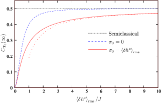
Figure 1: Saturation value of the triplet occupation probability $C_{T_{0}}(\infty)=\overline{C_{n}}$ vs. $\left\langle\delta h^{z}\right\rangle_{\mathrm{rms}}/J$ when the nuclear spin system has been squeezed into an eigenstate of $\delta h^{z}$ (dashed line) and when the state of the nuclear spin system describes a Gaussian distribution of eigenvalues $\delta h_{n}^{z}$, with mean $\overline{\delta h_{n}^{z}}=0$ and variance $\sigma_{0}^{2}=\overline{\left(\delta h_{n}^{z}\right)^{2}}$ (solid line). We also show the analytical asymptotics for $\sigma_{0}\gg J$, given by Eq. (15) (dotted line) and the semiclassical value ($C_{T_{0}}(\infty)=1/2$) (dash-dotted line).

Now we turn to the interference term $C_{T_{0}}^{\mathrm{int}}(t)$ given by Eq. (13), which can be evaluated explicitly in several interesting limits. First, in the limiting case of vanishing exchange $(J=0)$, we have $C(x)=\frac{1}{2}$ from (12). Direct integration of Eq. (13) then gives

$$C_{T_{0}}^{\mathrm{int}}(t)=-\frac{1}{2}\exp\left(-\frac{t^{2}}{2t_{0}^{2}}\right),\,t_{0}=\frac{1}{2\sigma_{0}},\,J=0.$$ (16)

For zero exchange interaction, the correlator decays purely as a Gaussian, with decoherence time $t_{0}=\frac{1}{2\sigma_{0}}\approx\frac{\sqrt{N}}{IA}$ for a typical asymmetric double quantum dot (see Appendix A). However, for arbitrary nonzero exchange interaction $J\neq 0$, we find the asymptotic form of the correlator at long times is given by (see Appendix C):

$$C_{T_{0}}^{\mathrm{int}}\left(t\right) \sim -\frac{\cos\left(Jt+\frac{3\pi}{4}\right)}{4\sigma_{0}\sqrt{J}t^{3/2}},$$ (18)

$$t\gg\max\left(\frac{1}{J},\frac{1}{2\sigma_{0}},\frac{J}{4\sigma_{0}^{2}}\right).$$

Thus, for arbitrarily small exchange interaction $J$, the asymptotic decay law of the correlator is modified from the Gaussian behavior of Eq. (16) to a (much slower) power law ($\sim 1/t^{3/2}$). We also note that the long-time correlator has a universal phase shift of $\frac{3\pi}{4}$, which is independent of any microscopic parameters. Our calculation therefore provides an example of interesting non-Markovian decay in an experimentally accessible system. Furthermore, the slow-down of the asymptotic decay suggests that the exchange interaction can be used to modify the form of decay, in addition to the decoherence time, through a narrowing of the distribution of eigenstates (see the discussion following Eq. (20) below). We have evaluated the full correlator $C_{T_{0}}(t)$ by numerical integration of Eq. (13) and plotted the results in Figure 2 along with the analytical asymptotic forms from (18).

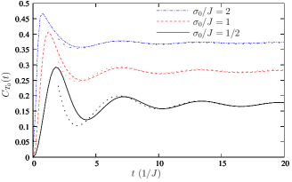
Figure 2: Decay of the correlator $C_{T_{0}}(t)$ evaluated by numerical integration of Eq. (13) for three ratios of $\sigma_{0}/J$: $\sigma_{0}/J=2$ (dashed-dotted line), $\sigma_{0}/J=1$ (dashed line), and $\sigma_{0}/J=1/2$ (solid line). The analytical long-time asymptotic expressions from Eq. (18) are shown as dotted lines.

We now investigate the relevant singlet-triplet correlator $C_{T_{0}}(t)$ in the limit of large exchange $J$. In this case, we have $x\lesssim\sigma_{0}\ll J$ for the typical $x$ contributing to the integral in Eq. (13). Thus, we can expand the prefactor $C(x)$ and frequency term in the integrand:

$$C(x) \approx 2\frac{x^{2}}{J^{2}},$$ (19)

$$\sqrt{J^{2}+4x^{2}} \approx J+2\frac{x^{2}}{J}.$$ (20)

From Eq. (20) it is evident that the range of frequencies that contribute to the correlator is suppressed by $\sigma_{0}/J$ (increasing the exchange narrows the distribution of eigenenergies that can contribute to decay). This narrowing of the linewidth will increase the decoherence time. Moreover, the leading-order $x^{2}$-dependence in (20) collaborates with the Gaussian distribution of $\delta h^{z}$ eigenstates to induce a power-law decay. With the approximations in Eqs. (19) and (20), we find an expression for the correlator that is valid for all times in the limit of large exchange $J$ by direct evaluation of the integral in Eq. (13):

$$C_{T_{0}}^{\mathrm{int}}(t) = -2\left(\frac{\sigma_{0}}{J}\right)^{2}\frac{\cos\left(Jt+\frac{3}{2}\arctan\left(\frac{t}{t_{0}^{\prime}}\right)\right)}{\left(1+\left(\frac{t}{t_{0}^{\prime}}\right)^{2}\right)^{3/4}},$$ (22)

$$t_{0}^{\prime}=\frac{J}{4\sigma_{0}^{2}},\,\,J\gg\sigma_{0}.$$

There is a new timescale ($t_{0}^{\prime}=J/4\sigma_{0}^{2}$) that appears for large $J$ due to dynamical narrowing; increasing the exchange $J$ results in rapid precession of the pseudospin $\boldsymbol{\tau}$ about the $z$-axis, which makes transverse fluctuations along $\tau^{x}$ due to $\delta h^{z}$ progressively unimportant. Explicitly, we have $t_{0}^{\prime}\approx JN/4A^{2}\gg\sqrt{N}/A$ for $J\gg\sigma_{0}\approx A/\sqrt{N}$.

Eq. (22) provides a potentially useful means of extracting the relevant microscopic parameters from an experiment. $J$ and $\sigma_{0}$ can be determined independent of each other exclusively from a measurement of the oscillation frequency and phase shift of $C_{T_{0}}^{\mathrm{int}}(t)$. In particular, any loss of oscillation amplitude (visibility) due to systematic error in the experiment can be ignored for the purposes of finding $\sigma_{0}$ and $J$. The loss in visibility can then be quantified by comparison with the amplitude expected from Eq. (22). We illustrate the two types of decay that occur for large and small $J$ in Figure 3.

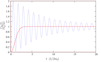
Figure 3: The correlator $C_{T_{0}}(t)/C_{T_{0}}(\infty)$ shows a rapid Gaussian decay when $J=0$ (solid line, from Eq. (16)), but has a much slower power-law decay $\sim 1/t^{3/2}$ for large exchange $J=10\sigma_{0}\gg\sigma_{0}$ (dotted line, from Eq. (22)).

II.1 Inhomogeneous polarization, $\overline{\delta h_{n}^{z}}\neq 0$

It is possible that a nonequilibrium inhomogeneous average polarization could be generated in the nuclear spin system, in which case $\overline{\delta h_{n}^{z}}\neq 0$. Pumping of nuclear spin polarization occurs naturally, for example, at donor impurities in GaAs during electron spin resonance (ESR), resulting in a shift of the ESR resonance condition.Seck et al. (1997) It is therefore important to investigate the effects of a nonzero average Overhauser field inhomogeneity on the decay law and timescale of the singlet-triplet correlator. In this subsection we generalize our previous results for the case $\overline{\delta h_{n}^{z}}\neq 0$.

We set the mean Overhauser field inhomogeneity to $\overline{\delta h_{n}^{z}}=x_{0}$, in which case the complex singlet-triplet interference term is given by

$$\tilde{C}_{T_{0}}^{\mathrm{int}}(t) = -\int_{-\infty}^{\infty}dxC(x)P_{\sigma_{0};x_{0}}(x)e^{it\sqrt{J^{2}+4x^{2}}}.$$ (23)

When the mean value of the Overhauser field inhomogeneity $x_{0}$ is much larger than the fluctuations $\sigma_{0}$ ($x_{0}\gg\sigma_{0}$), we approximate $C(x)\approx C(x_{0})$ and expand the frequency term $\sqrt{J^{2}+4x^{2}}=\omega_{0}+\frac{4x_{0}}{\omega_{0}}(x-x_{0})+\frac{2J^{2}}{\omega_{0}^{3}}(x-x_{0})^{2}+\cdots$, where $\omega_{0}=\sqrt{J^{2}+4x_{0}^{2}}$. We retain only linear order in $x-x_{0}$ for the frequency term, which is strictly valid for times $t\ll(J^{2}+4x_{0}^{2})^{3/2}/2J^{2}\sigma_{0}^{2}$. This time estimate is found by replacing $\left(x-x_{0}\right)^{2}\approx\sigma_{0}^{2}$ in the quadratic term and demanding that the quadratic term multiplied by time be much less than one. In this limit, the correlator and range of validity are then

$$C_{T_{0}}^{\mathrm{int}}(t) = -\frac{2x_{0}^{2}}{\omega_{0}^{2}}e^{-\frac{1}{2}\left(\frac{t}{t_{0}^{\prime\prime}}\right)^{2}}\cos\left(\omega_{0}t\right),$$ (26)

$$t_{0}^{\prime\prime}=\frac{\omega_{0}}{4x_{0}\sigma_{0}},\,\,\,\,\,\omega_{0}=\sqrt{J^{2}+4x_{0}^{2}},$$

$$x_{0}\gg\sigma_{0},\,\,\,\,\,t\ll\frac{\left(J^{2}+4x_{0}^{2}\right)^{3/2}}{2J^{2}\sigma_{0}^{2}}.$$

This expression is valid for any value of the exchange $J$, up to the timescale indicated.

In contrast with the previous result for $x_{0}=0$, from Eq. (26) we find that the long-time saturation value of the correlator deviates from the semiclassical result ($C_{T_{0}}(\infty)=-C_{T_{0}}^{\mathrm{int}}(0)=1/2$) by an amount that is quadratic in the exchange $J$ for $J\ll x_{0}$:

$$C_{T_{0}}(\infty)=C_{T_{0}}^{\mathrm{int}}(0)\sim\left\{\begin{array}[]{c}\frac{1}{2}-\frac{1}{8}\left(\frac{J}{x_{0}}\right)^{2},\,\,J\ll x_{0},\\ 2\left(\frac{x_{0}}{J}\right)^{2},\,\,J\gg x_{0}.\end{array}\right.,\,\,\,\,\,x_{0}\gg\sigma_{0}.$$ (27)

In the limit of large exchange, $J\gg\max\left(\sigma_{0},x_{0}\right)$, we can once again apply the approximations given in Eqs. (19) and (20). Using these approximations in Eq. (23) and integrating then gives

$$\tilde{C}_{T_{0}}^{\mathrm{int}}(t) = -2\left(\frac{\sigma_{0}}{J}\right)^{2}\xi^{3}(t)\left(1+\left(\frac{x_{0}}{\sigma_{0}}\right)^{2}\xi^{2}(t)\right)\exp\left\{iJt-\frac{x_{0}^{2}}{2\sigma_{0}^{2}}\left(1-\xi^{2}(t)\right)\right\},$$ (29)

$$\xi(t)=\left(1-i\frac{t}{t_{0}^{\prime}}\right)^{-1/2},\,\,t_{0}^{\prime}=\frac{J}{4\sigma_{0}^{2}},\,\,\,\,\,J\gg\max(x_{0},\sigma_{0}),\,\,t\ll\frac{J^{3}}{2\max\left(x_{0}^{4},\sigma_{0}^{4}\right)}.$$

We have found the limit on the time range of validity in Eq. (29) using the same estimate that was used for Eqs. (26-26). At short times, $t\ll t_{0}^{\prime}=J/4\sigma_{0}^{2}$, we expand $\xi^{2}(t)\approx 1+i\frac{t}{t_{0}^{\prime}}-\left(\frac{t}{t_{0}^{\prime}}\right)^{2}$ and find that this function decays initially as a Gaussian with timescale $t_{0}^{\prime\prime}\approx J/4x_{0}\sigma_{0}$:

$$C_{T_{0}}^{\mathrm{int}}(t) \sim -2\frac{\sigma_{0}^{2}+x_{0}^{2}}{J^{2}}e^{-\frac{1}{2}\left(\frac{t}{t_{0}^{\prime\prime}}\right)^{2}}\cos\left(\omega_{0}^{\prime}t\right),$$ (32)

$$t_{0}^{\prime\prime}\approx\frac{J}{4x_{0}\sigma_{0}},\,\,\,\,\,\omega_{0}^{\prime}=J+\frac{2x_{0}^{2}}{J},$$

$$t\ll t_{0}^{\prime}=\frac{J}{4\sigma_{0}^{2}},\,\,\,\,\,J\gg\max(x_{0},\sigma_{0}).$$

This agrees with the result in Eq. (26) when $J\gg x_{0}\gg\sigma_{0}$.

For sufficiently large exchange $J$, the expression given by Eq. (29) is valid for times longer than the previous expression, given by Eq. (26). We perform an asymptotic expansion of Eq. (29) for long times using $\xi(t\gg t_{0}^{\prime})\sim e^{i\pi/4}\sqrt{t_{0}^{\prime}/t}$. This gives

$$C_{T_{0}}^{\mathrm{int}}(t) \sim -\frac{e^{-x_{0}^{2}/2\sigma_{0}^{2}}\cos(Jt+\frac{3\pi}{4})}{4\sigma_{0}\sqrt{J}t^{3/2}},$$ (34)

$$t\gg t_{0}^{\prime}=\frac{J}{4\sigma_{0}^{2}},\,\,\,\,\,J\gg\max(x_{0},\sigma_{0}).$$

As in the case of $x_{0}=0$, the long-time asymptotics of Eq. (29) once again give a power law $\sim 1/t^{3/2}$, although the amplitude of the long-time decay is exponentially suppressed in the ratio $x_{0}^{2}/\sigma_{0}^{2}$. When $x_{0}=0$, Eq. (34) recovers the previous result, given in Eq. (18).

II.2 Reducing decoherence

The results of this section suggest a general strategy for increasing the amplitude of coherent oscillations between the singlet $\left|S\right\rangle$ and triplet $\left|T_{0}\right\rangle$ states, and for weakening the form of decay. To avoid a rapid Gaussian decay with a timescale $t_{0}^{\prime\prime}=J/4x_{0}\sigma_{0}$, the mean Overhauser field inhomogeneity should be made smaller than the fluctuations ($\overline{\delta h_{n}^{z}}=x_{0}\lesssim\sigma_{0}$) and the exchange $J$ should be made larger than $x_{0}$ and $\sigma_{0}$ ($J\gg\max(x_{0},\sigma_{0})$). Explicitly, the ideal condition for slow and weak (power-law) decay can be written as

$$J\gg\sigma_{0}\gtrsim x_{0}.$$ (35)

The condition in Eq. (35) can be achieved equally well by increasing the exchange coupling $J$ for fixed hyperfine fluctuations $\sigma_{0}$ or by reducing the fluctuations $\sigma_{0}$ through state squeezing or by making the double-dot confining potential more symmetric (see Appendix A).

III Dynamics in the subspace of $\left|S\right\rangle$ and $\left|T_{+}\right\rangle$

We now consider the case when the Zeeman energy of the $S^{z}=1$ triplet state approximately compensates the exchange ($\left|\Delta\right|\ll J$, where $\Delta=\epsilon_{z}+J$). In addition, we assume the exchange is much larger than the nuclear field energy scales $J\gg\mathrm{max}\left\{\left\langle\mathbf{\delta h}\right\rangle_{\mathrm{rms}},\left\langle\mathbf{h}\right\rangle_{\mathrm{rms}}\right\}$. Under these conditions, we consider the dynamics in a subspace formed by the singlet $\left|S\right\rangle\to\left|\tau^{z}=-1\right\rangle$ and the $S^{z}=1$ triplet state $\left|T_{+}\right\rangle\to\left|\tau^{z}=+1\right\rangle$, governed by the Hamiltonian (to zeroth order in $1/J$, see Appendix B):

$$H_{+}=\frac{1}{2}\left(\Delta+h^{z}\right)\left(1+\tau^{z}\right)-\frac{1}{\sqrt{2}}\left(\delta h^{-}\tau^{+}+\mathrm{H.c.}\right).$$ (36)

Here, $\delta h^{\pm}=\delta h^{x}\pm i\delta h^{y}$ and $\tau^{\pm}=\frac{1}{2}\left(\tau^{x}\pm i\tau^{y}\right)$. The $\left|T_{+}\right\rangle$ probability at time $t>0$ is

$$C_{T_{+}}(t)=\sum_{n,n^{\prime}}\rho_{I}(n)\left|\left\langle n^{\prime}\right|\otimes\left\langle T_{+}\right|e^{-iH_{+}t}\left|S\right\rangle\otimes\left|n\right\rangle\right|^{2}.$$ (37)

This case is essentially different from the previous one, since the eigenstates of $H_{+}$ are no longer simply product states of electron and nuclear spin, implying a back-action of the electron on the nuclear system. Nevertheless, when $\left\langle h^{z}+\Delta\right\rangle_{\mathrm{rms}}\gg\left\langle\mathbf{\delta h^{\pm}}\right\rangle_{\mathrm{rms}}$, we can evaluate the correlator in standard time-dependent perturbation theory to leading order in the term $V=-\frac{1}{\sqrt{2}}\left(\tau^{+}\delta h^{-}+\tau^{-}\delta h^{+}\right)$. Neglecting corrections of order $h_{n}^{z}/\Delta\ll 1$, this gives

$$C_{T_{+}}^{(2)}(t)\approx\overline{\frac{\alpha_{n}^{2}}{\Delta^{2}}\left(1-\cos\left(\left[\left[h^{z}\right]_{n}+\Delta\right]t\right)\right)},$$ (38)

where $\alpha_{n}=\sum_{n^{\prime}}\left|\left\langle n^{\prime}\right|\delta h^{-}\left|n\right\rangle\right|^{2}$, and $\left|n\right\rangle$ is now an eigenstate of the operator $h^{z}$ with eigenvalue $\left[h^{z}\right]_{n}$. To estimate the size of $\alpha_{n}$, we assume identical completely decoupled dots and nuclear polarization $p\ll 1$, which gives $\alpha_{n}^{2}\approx\frac{1}{2}I(I+1)\sum_{k}A_{k}^{2}$, where $A_{k}$ is the hyperfine coupling constant to the nuclear spin at lattice site $k$ (with total nuclear spin $I$) and the sum $\sum_{k}$ runs over all lattice sites in one of the dots. We estimate the typical size of $\alpha_{n}$ with the replacements $A_{k}\to\frac{A}{N},\,\sum_{k}\to N$, which gives $\alpha_{n}\approx\alpha/\sqrt{2}=\sqrt{\frac{I(I+1)}{2N}}A$, where $N$ characterizes the number of nuclear spins within the dot envelope wavefunction. If we assume the nuclear spin state is described by a continuous Gaussian distribution of $h^{z}$ eigenstates with mean $\overline{h_{n}^{z}}=0$ and variance $\sigma_{+}^{2}$, we find

$$C_{T_{+}}^{(2)}(t)\approx\frac{1}{2}\left(\frac{\alpha}{\Delta}\right)^{2}\left(1-e^{-t^{2}/2t_{+}^{2}}\cos\left(\Delta t\right)\right),\,\,\,\,t_{+}=\frac{1}{2\sigma_{+}}.$$ (39)

Thus, if we ignore any possibility for recurrence, the distribution of $h^{z}$ eigenstates will lead to Gaussian decay of the two-electron spin state, as is the case for a single electron.Schliemann et al. (2002); Coish and Loss (2004) However, as in the case of a single electron, this decay can be reduced or eliminated altogether by narrowing the distribution of $h^{z}$ eigenstates $\left|n\right\rangle$ through measurement (squeezing the nuclear spin state).Coish and Loss (2004) We show these two cases (with and without squeezing of the nuclear state) in Figure 4.

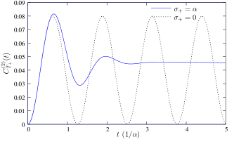
Figure 4: Decay of the correlator $C_{T_{+}}(t)$ in two cases. A typical unprepared initial state, where the nuclear spin system is in a superposition of $h^{z}$ eigenstates, results in a Gaussian decay (solid line, from Eq. (39)). If the nuclear spin state is squeezed into an $h^{z}$ eigenstate, there is no decay, only coherent oscillations (dotted line, from Eq. (38)). For this plot we have used $\Delta=5\alpha$.

IV Singlet-triplet decoherence due to orbital dephasing

To this point we have neglected dephasing of the singlet $\left|S\right\rangle$ and triplet $\left|T_{j}\right\rangle$ $(j=0,+)$ states due to coupling in the orbital sector. The effective Hamiltonian description ignores the different character of the orbital states for singlet and triplet, and so it is tempting to assume that orbital dephasing is unimportant where the effective Hamiltonian is valid. However, the singlet and triplet do have different orbital states which can, in general, couple differently to the environment through the charge degree of freedom, and therefore acquire different phases. Examples of such environmental influences are charge fluctuators or measurement devices, such as quantum point contacts used for charge readout.Engel et al. (2004); Elzerman et al. (2004) Here we briefly step away from the effective Hamiltonians derived in Appendix B to give a physical picture of the effects of orbital dephasing in terms of the true double-dot wavefunctions. We then return to the effective Hamiltonian picture in order to give a more general estimate of the effects of orbital dephasing on singlet-triplet decoherence for a two-electron double dot.

We consider a double quantum dot containing a fixed (quantized) number of electrons $N$. Within the far-field approximation, the double-dot charge distribution couples to the environment first through a monopole, and then a dipole term. Since the charge on the double dot is quantized, the monopole term gives an equal contribution for both the singlet and triplet wavefunctions. The leading interaction that can distinguish singlet from triplet is the electric dipole term:

$$V_{\mathrm{orb}}(t)\approx-\mathbf{p}_{N}\cdot\mathbf{E}(t).$$ (40)

Here, $\mathbf{p}_{N}$ is the electric dipole moment operator for the charge distribution in a double dot containing $N$ electrons and $\mathbf{E}(t)$ is a fluctuating electric field due to the surrounding environment, which we model by a Gaussian random process. For a double quantum dot with well-localized single-particle eigenstates we denote the charge states by $\left|(n,m)\right\rangle$, indicating that the double-dot has $n$ electrons in dot $1$ and $m$ electrons in dot $2$, where $n+m=N$. If the double dot contains only a single electron $(N=1)$, the environment can distinguish the two localized states through the difference in the dipole moment operator, which has the size $\left|\Delta\mathbf{p}_{1}\right|=\left|\left\langle(1,0)\right|\mathbf{p}_{1}\left|(1,0)\right\rangle-\left\langle(0,1)\right|\mathbf{p}_{1}\left|(0,1)\right\rangle\right|\approx 2\left|e\right|a$, where $e$ is the electron charge and $2a$ is the inter-dot spacing. When $N=2$, for highly-localized states, only the states with double-occupancy ($\left|(0,2)\right\rangle$ and $\left|(2,0)\right\rangle$) contribute to the dipole moment. If the typical hyperfine energy scale is much smaller than the detuning from resonance $\delta$ of the $\left|(1,1)\right\rangle$ and $\left|(0,2)\right\rangle$ states ($\max\left(\left\langle\delta\mathbf{h}\right\rangle_{\mathrm{rms}},\left\langle\mathbf{h}\right\rangle_{\mathrm{rms}}\right)\ll\delta$), only the $\left|(1,1)\right\rangle$ singlet state (not the triplets) will mix with the doubly-occupied states, so the singlet and triplet states will be energetically distinguishable through $\left|\Delta\mathbf{p}_{2}\right|=\left|\left\langle S\right|\mathbf{p}_{2}\left|S\right\rangle\right|\approx 2\left|e\right|a\left|P_{(0,2)}-P_{(2,0)}\right|\lesssim 2\left|e\right|aD$, where $P_{(0,2)}$ $\left(P_{(2,0)}\right)$ is the probability to find the singlet $\left|S\right\rangle$ in the $\left|(0,2)\right\rangle$ $(\left|(2,0)\right\rangle)$ state and $D=P_{(0,2)}+P_{(2,0)}$ is the double occupancy. In this discussion, we assume that the exchange is much larger than the hyperfine energy scales, $J\gg\max\left(\left\langle\mathbf{h}\right\rangle_{\mathrm{rms}},\left\langle\delta\mathbf{h}\right\rangle_{\mathrm{rms}}\right)$, so that the singlet and triplet states are good approximates for the true two-electron eigenstates.

For weak coupling to the environment, and assuming the environment correlation time is much less than the orbital dephasing time $t_{\phi}^{(N)}$, we can apply standard techniques to determine the dephasing time for a two-level system described by the Bloch equations.Blum (1981) We find that the fluctuations in $\mathbf{E}(t)$ lead to exponential dephasing with the rate $1/t_{\phi}^{(N)}=\frac{1}{4}\left|\Delta\mathbf{p}_{N}\right|^{2}\int_{-\infty}^{\infty}dtE(t)E(0)$, where the scalar $E(t)$ is the component of $\mathbf{E}(t)$ along $\Delta\mathbf{p}_{N}$ and we assume $\lim_{t\to\infty}\frac{1}{t}\int_{0}^{t}dt^{\prime}E(t^{\prime})=0$. Assuming equivalent environments for the single-particle and two-particle cases, the ratio of the single-particle to two-particle dephasing times is then

$$\frac{t_{\phi}^{(1)}}{t_{\phi}^{(2)}}=\left|\frac{\Delta\mathbf{p}_{2}}{\Delta\mathbf{p}_{1}}\right|^{2}\lesssim D^{2}.$$ (41)

The single-electron orbital dephasing rate has been measured to be $t_{\phi}^{(1)}\approx 1\,\mathrm{ns}$Hayashi et al. (2003) and $t_{\phi}^{(1)}\approx 400\,\mathrm{ps}$Petta et al. (2004b) in different gated double quantum dots. If the hyperfine interaction (which becomes important on the timescale $t\gtrsim 5\,\mathrm{ns}$) is to provide the major source of decoherence in these two-electron structures, we therefore require $t_{\phi}^{(2)}\gg t_{\phi}^{(1)}$. This condition can be achieved by ensuring a small double occupancy $D\ll 1$ of the singlet state. When the inter-dot tunnel coupling $t_{12}$ is much less than the detuning from resonance $\delta$ ($t_{12}\ll\delta\ll U+U^{\prime}$, with on-site and nearest-neighbor charging energies $U$ and $U^{\prime}$, respectively – see Appendix B) we find the double-occupancy of $\left|S\right\rangle$ in perturbation theory is

$$D\approx 2\left(\frac{t_{12}}{\delta}\right)^{2}\ll 1.$$ (42)

Even in this regime, orbital dephasing may become the limiting timescale for singlet-triplet decoherence after the removal of hyperfine-induced decoherence by spin echo. A detailed analysis of the double-occupancy and its relation to the concurrence (an entanglement measure) for a symmetric double dot can be found in Refs. Golovach and Loss, 2003, 2004.

With this physical picture in mind, we can generalize the above results to the case when the electrons experience fluctuations due to any time-dependent classical fields. In particular, if the separation in single-particle energy eigenstates for $N=1$ is $\epsilon+\delta\epsilon(t)$, where $\delta\epsilon(t)$ fluctuates randomly with amplitude $\delta\epsilon$, and similarly, if for $N=2$ the singlet and triplet levels are separated by an exchange $J+\delta J(t)$, where $\delta J(t)$ has amplitude $\delta J$, we find

$$\frac{t_{\phi}^{(1)}}{t_{\phi}^{(2)}}=\left|\frac{\delta J}{\delta\epsilon}\right|^{2}.$$ (43)

From this expression we conclude that the optimal operating point of the double dot is where the slope of $J$ vs. $\epsilon$ vanishes, i.e., $\delta J/\delta\epsilon=0$. At this optimal point, $t_{\phi}^{(2)}\to\infty$, within the approximations we have made. Eq. (43) is valid for weak coupling to the environment (i.e. $\delta J\ll J$ and $\delta\epsilon\ll\epsilon$), and when the environment correlation time is small compared to the dephasing times. If, for example, we take $J\approx 2t_{12}^{2}/\delta$ for $U+U^{\prime}\gg\delta\gg t_{12}$ from Eq. (58) and if $\delta\epsilon$ corresponds to fluctuations in the single-particle charging energy difference ($\epsilon\sim(V_{g1}-V_{g2})\sim\delta$ from Eq. (56)), we find $t_{\phi}^{(1)}/t_{\phi}^{(2)}\approx 4t_{12}^{4}/\delta^{4}$, in agreement with Eqs. (41) and (42). In particular, the hyperfine-dominated singlet-triplet decoherence becomes visible when $t_{\phi}^{(2)}\gg t_{0}^{\prime},\,t_{0}^{\prime\prime}\gg t_{0},\,t_{+}$. This regime is achievable by choosing $\delta\gg t_{12}$, but still $J\approx 2t_{12}^{2}/\delta\gg\sigma_{0}$, since $t_{\phi}^{(2)}$ is a much stronger function of $\delta$ than $t_{0}^{\prime},\,t_{0}^{\prime\prime}$. That is, the two-particle dephasing time scales like $t_{\phi}^{(2)}\sim\delta^{4}$, but the typical hyperfine-induced decay times scale like $t_{0}^{\prime},t_{0}^{\prime\prime}\sim J\sim 1/\delta$. On the other hand, when $t_{12}\approx\delta$, we have $\left|\delta J/\delta\epsilon\right|\sim O(1)$, which gives $t_{\phi}^{(2)}\sim t_{\phi}^{(1)}$, and thus a very short singlet-triplet decoherence time ($\approx 1\,\mathrm{ns}$), which is dominated by orbital dephasing.

V Conclusions

We have shown that a fully quantum mechanical solution is possible for the dynamics of a two-electron system interacting with an environment of nuclear spins under an applied magnetic field. Our solution shows that the singlet-triplet correlators $C_{T_{0}}(t)$ and $C_{T_{+}}(t)$ will decay due to the quantum distribution of the nuclear spin system, even for a nuclear system that is static. We have found that the asymptotic behavior of $C_{T_{0}}(t)$ undergoes a transition from Gaussian to power-law ($\sim 1/t^{3/2}$) when the Heisenberg exchange coupling $J$ becomes nonzero, and acquires a universal phase shift of $3\pi/4$. The oscillation frequency and phase shift as a function of time can be used to determine the exchange and Overhauser field fluctuations. We have also investigated the effects of an inhomogeneous polarization on $C_{T_{0}}(t)$, and have suggested a general strategy for reducing decoherence in this system. Finally, we have discussed orbital dephasing and its effect on singlet-triplet decoherence.

Appendix A Estimating the Overhauser field

In this appendix we estimate the size of the Overhauser field inhomogeneity for a typical double quantum dot, and show that this quantity depends, in a sensitive way, on the form of the orbital wavefunctions.

As in the main text, we take the average Overhauser field and the Overhauser field inhomogeneity to be $\mathbf{h}=\frac{1}{2}\left(\mathbf{h}_{1}+\mathbf{h}_{2}\right)$ and $\delta\mathbf{h}=\frac{1}{2}\left(\mathbf{h}_{1}-\mathbf{h}_{2}\right)$ respectively, where $\mathbf{h}_{l}=Av\sum_{k}\left|\psi_{0}^{l}(\mathbf{r}_{k})\right|^{2}\mathbf{I}_{k}$, and $\psi_{0}^{l}(\mathbf{r})$ is orbital eigenstate $l$ in the double quantum dot. In the presence of tunneling, the eigenstates of a symmetric double quantum dot will be well-describedBurkard et al. (1999); Golovach and Loss (2004) by the symmetric and antisymmetric linear combination of dot-localized states $\phi_{l}(\mathbf{r}),\,l=1,2$: $\psi_{0}^{1,2}(\mathrm{r})=\frac{1}{\sqrt{2}}\left(\phi_{1}(\mathrm{r})\pm\phi_{2}(\mathrm{r})\right)$. In this case, we find

$$\left\langle\delta\mathbf{h}\right\rangle_{\mathrm{rms}}=Av\left\langle\sum_{k}\mathrm{Re}\left[\phi_{1}^{*}(\mathbf{r}_{k})\phi_{2}(\mathbf{r}_{k})\right]\mathbf{I}_{k}\right\rangle_{\mathrm{rms}}.$$ (44)

We take $\left\langle\frac{1}{N}\sum_{k}\mathbf{I}_{k}\right\rangle_{\mathrm{rms}}\approx\sqrt{I(I+1)/N}$ to be the r.m.s. value for a system of $N$ nuclear spins with uniform polarization $p\ll 1$. Changing the sum to an integral according to $v\sum_{k}\to\int d^{3}r$ then gives

$$\left\langle\delta\mathbf{h}\right\rangle_{\mathrm{rms}}\approx\gamma\sqrt{\frac{I(I+1)}{N}}A=\gamma\alpha,$$ (45)

where $\gamma=\int d^{3}r\,\mathrm{Re}\left[\phi_{1}^{*}(\mathbf{r})\phi_{2}(\mathbf{r})\right]$ is the overlap of the localized orbital dot states and we have introduced the energy scale $\alpha=\sqrt{I(I+1)}A/\sqrt{N}$. The result in Eq. (45) suggests that the Overhauser field inhomogeneity can be drastically reduced in a symmetric double quantum dot simply by separating the two dots, reducing the wavefunction overlap. If, however, the double dot is sufficiently asymmetric, the correct orbital eigenstates will be well-described by localized states $\psi_{0}^{l}(\mathrm{r})=\phi_{l}(\mathrm{r}),\,\,l=1,2$, (with overlap $\gamma\ll 1$), in which case we find

$$\left\langle\delta\mathbf{h}\right\rangle_{\mathrm{rms}}\approx\sqrt{\frac{I(I+1)}{N}}A=\alpha.$$ (46)

Thus, great care should be taken in determining $\left\langle\delta\mathbf{h}\right\rangle_{\mathrm{rms}}$ based on microscopic parameters. In particular, for a symmetric double quantum dot, the overlap $\gamma$ must also be known to determine $\left\langle\delta\mathbf{h}\right\rangle_{\mathrm{rms}}$ based on $N$.

In contrast, for the total Overhauser operator $\mathbf{h}$, in both of the above cases ($\psi_{0}^{1,2}(\mathrm{r})=\frac{1}{\sqrt{2}}\left(\phi_{1}(\mathrm{r})\pm\phi_{2}(\mathrm{r})\right)$ or $\psi_{0}^{l}(\mathrm{r})=\phi_{l}(\mathrm{r}),\,\,l=1,2$), we find

$$\left\langle\mathbf{h}\right\rangle_{\mathrm{rms}}\approx\sqrt{\frac{I(I+1)}{N}}A=\alpha.$$ (47)

Appendix B Effective Hamiltonians for two-electron states in a double quantum dot

In this appendix we derive effective Hamiltonians for a two-electron system interacting with nuclear spins in a double quantum dot via the contact hyperfine interaction.

We begin from the two-electron Hamiltonian in second-quantized form,

$$H=H_{SP}+H_{C}+H_{T}+H_{Z}+H_{\mathrm{hf}},$$ (48)

where $H_{SP}$ describes the single-particle charging energy, $H_{C}$ models the Coulomb interaction between electrons in the double dot, $H_{T}$ describes tunneling between dot orbital states, $H_{Z}$ gives the electron Zeeman energy (we neglect the nuclear Zeeman energy, which is smaller by the ratio of nuclear to Bohr magneton: $\mu_{N}/\mu_{B}\sim 10^{-3}$) and $H_{\mathrm{hf}}$ describes the Fermi contact hyperfine interaction between electrons on the double dot and nuclei in the surrounding lattice. Explicitly, these terms are given by

$$H_{SP} = \sum_{l\sigma}V_{gl}n_{l\sigma};\,\,\,\,\,n_{l\sigma}=d_{l\sigma}^{\dagger}d_{l\sigma},$$ (49)

$$H_{C} = U\sum_{l}n_{l\uparrow}n_{l\downarrow}+U^{\prime}(n_{1\uparrow}+n_{1\downarrow})(n_{2\uparrow}+n_{2\downarrow}),$$ (50)

$$H_{T} = t_{12}\sum_{\sigma}\left(d_{1\sigma}^{\dagger}d_{2\sigma}+d_{2\sigma}^{\dagger}d_{1\sigma}\right),$$ (51)

$$H_{Z} = \frac{\epsilon_{z}}{2}\sum_{l}(n_{l\uparrow}-n_{l\downarrow}),$$ (52)

$$H_{\mathrm{hf}} = \sum_{l}\mathbf{S}_{l}\cdot\mathbf{h}_{l};\,\,\,\,\,\mathbf{S}_{l}=\frac{1}{2}\sum_{\sigma\sigma^{\prime}}d_{l\sigma}^{\dagger}\boldsymbol{\sigma}_{\sigma\sigma^{\prime}}d_{l\sigma^{\prime}}.$$ (53)

Here, $d_{l\sigma}^{\dagger}$ creates an electron with spin $\sigma$ in orbital state $l$ $(l=1,2)$, $V_{gl}$ is the single-particle charging energy for orbital state $l$, $U$ is the two-particle charging energy for two electrons in the same orbital state, and $U^{\prime}$ is the two-particle charging energy when there is one electron in each orbital. When the orbital eigenstates are localized states in quantum dot $l=1,2$, $V_{gl}$ is supplied by the back-gate voltage on dot $l$ and $U$ $(U^{\prime})$ is the on-site (nearest-neighbor) charging energy. $t_{12}$ is the hopping matrix element between the two orbital states, $\epsilon_{z}$ is the electron Zeeman splitting, $\mathbf{h}_{l}$ is the nuclear field (Overhauser operator) for an electron in orbital $l$, and $\boldsymbol{\sigma}_{\sigma\sigma^{\prime}}$ gives the matrix elements of the vector of Pauli matrices $\boldsymbol{\sigma}=(\sigma_{x},\sigma_{y},\sigma_{z})$. In the subspace of two electrons occupying two orbital states, the spectrum of $H_{SP}+H_{C}$ consists of four degenerate “delocalized” states with one electron in each orbital, all with unperturbed energy $E_{(1,1)}$ (a singlet $\left|S(1,1)\right\rangle$ and three triplets: $\left|T_{j}(1,1)\right\rangle;\,j=\pm,0$), and two non-degenerate “localized” singlet states $\left|S(2,0)\right\rangle$ and $\left|S(0,2)\right\rangle$, with two electrons in orbital $l=1$ or $l=2$, having energy $E_{(2,0)}$ and $E_{(0,2)}$, respectively.

To derive an effective Hamiltonian $H_{\mathrm{eff}}$ from a given Hamiltonian $H$, which has a set of nearly degenerate levels $\left\{\left|i\right\rangle\right\}$, we use the standard procedureStoneham (1975),

$$H_{\mathrm{eff}}=PHP+PHQ\frac{1}{E-QHQ}QHP,$$ (54)

where $P=\sum_{i}\left|i\right\rangle\left\langle i\right|$ is a projection operator onto the relevant subspace and $Q=1-P$ is its complement.

We choose the arbitrary zero of energy such that $E_{(1,1)}=V_{g1}+V_{g2}+U^{\prime}=0$ and introduce the detuning parameters

$$\delta_{1} = E_{(1,1)}-E_{(2,0)}=-2V_{g1}-U=-\delta-U-U^{\prime},$$ (55)

$$\delta_{2} = E_{(1,1)}-E_{(0,2)}=-2V_{g2}-U=\delta.$$ (56)

We then project onto the four-dimensional subspace formed by the delocalized singlet $\left|S(1,1)\right\rangle$ and three delocalized triplet states $\left|T_{j}(1,1)\right\rangle,\,\,\,\,\,j=\pm,0$. That is, we choose $Q=\left|S(0,2)\right\rangle\left\langle S(0,2)\right|+\left|S(2,0)\right\rangle\left\langle S(2,0)\right|$, $P=1-Q$. When $\delta_{1},\delta_{2}\gg t_{12}$, we have $E\approx E_{(1,1)}=0$ in the denominator of Eq. (54). This gives an effective spin Hamiltonian in the subspace of one electron in each orbital state:

$$H_{\mathrm{eff}} = \epsilon_{z}\sum_{l}S_{l}^{z}+\sum_{l}\mathbf{h}_{l}\cdot\mathbf{S}_{l}-J\left(\frac{1}{4}-\mathbf{S}_{1}\cdot\mathbf{S}_{2}\right),$$ (58)

$$J\approx-2t_{12}^{2}\left(\frac{1}{\delta}-\frac{1}{\delta+U+U^{\prime}}\right).$$

This Hamiltonian is more conveniently rewritten in terms of the sum and difference vectors of the electron spin and Overhauser operators $\mathbf{S}=\mathbf{S}_{1}+\mathbf{S}_{2},\,\,\,\,\,\delta\mathbf{S}=\mathbf{S}_{1}-\mathbf{S}_{2}$ and $\mathbf{h}=\frac{1}{2}\left(\mathbf{h}_{1}+\mathbf{h}_{2}\right),\,\,\,\,\,\delta\mathbf{h}=\frac{1}{2}\left(\mathbf{h}_{1}-\mathbf{h}_{2}\right)$:

$$H_{\mathrm{eff}} = \epsilon_{z}S^{z}+\mathbf{h}\cdot\mathbf{S}+\delta\mathbf{h}\cdot\delta\mathbf{S}+\frac{J}{2}\mathbf{S}\cdot\mathbf{S}-J.$$ (59)

Neglecting the constant term, in the basis of singlet and three triplet states, $\left\{\left|S(1,1)\right\rangle=\left|S\right\rangle,\left|T_{j}(1,1)\right\rangle=\left|T_{j}\right\rangle,\,j=\pm,0\right\}$, the Hamiltonian matrix for $H_{\mathrm{eff}}$ takes the form

$$\left(\begin{array}[]{cccc}0&-\delta h^{+}/\sqrt{2}&\delta h^{z}&\delta h^{-}/\sqrt{2}\\ -\delta h^{-}/\sqrt{2}&J+\epsilon_{z}+h^{z}&h^{-}/\sqrt{2}&0\\ \delta h^{z}&h^{+}/\sqrt{2}&J&h^{-}/\sqrt{2}\\ \delta h^{+}/\sqrt{2}&0&h^{+}/\sqrt{2}&J-\epsilon_{z}-h^{z}\end{array}\right),$$ (60)

where $\delta h^{\pm}=\delta h^{x}\pm i\delta h^{y}$ and $h^{\pm}=h^{x}\pm ih^{y}$. We are interested in this Hamiltonian in two limiting cases, where it becomes block-diagonal in a two-dimensional subspace.

B.1 Effective Hamiltonian in the $\left|S\right\rangle-\left|T_{0}\right\rangle$ subspace

Projecting $H$ onto the two-dimensional subspace spanned by $\left|T_{0}\right\rangle\to\left|\tau^{z}=+1\right\rangle$ and $\left|S\right\rangle\to\left|\tau^{z}=-1\right\rangle$, we find

$$H_{0}=N_{0}+\frac{1}{2}\mathbf{v}_{0}\cdot\boldsymbol{\tau},$$ (61)

where $\boldsymbol{\tau}=(\tau^{x},\tau^{y},\tau^{z})$ is a vector of Pauli matrices. The leading and first subleading corrections to $H_{0}$ in powers of $1/\epsilon_{z}$ are ($H_{0}=H_{0}^{(0)}+H_{0}^{(1)}+\cdots$, $H_{0}^{(i)}=N_{0}^{(i)}+\mathbf{v}_{0}^{(i)}$):

$$N_{0}^{(0)} = \frac{J}{2},$$ (62)

$$v_{0}^{z(0)} = J,$$ (63)

$$v_{0}^{+(0)} = 2\delta h^{z},$$ (64)

$$N_{0}^{(1)} = \frac{1}{4\epsilon_{z}}\left(\left[h^{-},h^{+}\right]+\left[\delta h^{-},\delta h^{+}\right]\right),$$ (65)

$$v_{0}^{z(1)} = \frac{1}{2\epsilon_{z}}\left(\left[h^{-},h^{+}\right]-\left[\delta h^{-},\delta h^{+}\right]\right),$$ (66)

$$v_{0}^{+(1)} = \frac{1}{\epsilon_{z}}\left(\delta h^{+}h^{-}+\delta h^{-}h^{+}\right).$$ (67)

Here, $\mathbf{N}_{X}=(N_{X}^{x},N_{X}^{y},N_{X}^{z})$, $\mathbf{v}_{X}=(v_{X}^{x},v_{X}^{y},v_{X}^{z})$, $N_{X}^{\pm}=N_{X}^{x}\pm iN_{X}^{y}$, and $v_{X}^{\pm}=v_{X}^{x}\pm iv_{X}^{y}$. For a typical unpolarized system, we estimate the size of all subleading corrections from their r.m.s. expectation values, taken with respect to an unpolarized nuclear state. This gives

$$\left\langle H_{0}^{(1)}\right\rangle_{\mathrm{rms}}=O\left(\frac{\alpha^{2}}{\epsilon_{z}}\right),$$ (68)

where $\alpha$ is given by $\alpha=\sqrt{I(I+1)}A/\sqrt{N}$ (for a GaAs quantum dot containing $N\approx 10^{5}$ nuclear spins, $1/\alpha\approx 5\,\mathrm{ns}$). We therefore expect dynamics calculated under $H_{0}^{(0)}$ to be valid up to timescales on the order of $\epsilon_{z}/\alpha^{2}\gg 1/\alpha$, when $\epsilon_{z}\gg\alpha$.

B.2 Effective Hamiltonian in the $\left|S\right\rangle-\left|T_{+}\right\rangle$ subspace

When the Zeeman energy of the $\left|T_{+}\right\rangle$ triplet state approximately compensates the exchange, $\max\left(\left\langle\mathbf{h}\right\rangle_{\mathrm{rms}},\left\langle\delta\mathbf{h}\right\rangle_{\mathrm{rms}},\left|\Delta\right|\right)\ll J$ (where $\Delta=\epsilon_{z}+J$), we find an effective Hamiltonian in the subspace $\left|T_{+}\right\rangle\to\left|\tau^{z}=+1\right\rangle,\,\left|S\right\rangle\to\left|\tau^{z}=-1\right\rangle$:

$$H_{+}=N_{+}+\frac{1}{2}\mathbf{v}_{+}\cdot\boldsymbol{\tau},$$ (69)

where the leading and subleading corrections in powers of $1/J$ are

$$N_{+}^{(0)} = \frac{1}{2}\left(\Delta+h^{z}\right),$$ (70)

$$v_{+}^{z(0)} = \Delta+h^{z},$$ (71)

$$v_{+}^{+(0)} = -\sqrt{2}\delta h^{+},$$ (72)

$$N_{+}^{(1)} = -\frac{1}{2J}\left(\left(\delta h^{z}\right)^{2}+\frac{1}{4}\delta h^{-}\delta h^{+}+\frac{1}{2}h^{-}h^{+}\right),$$ (73)

$$v_{+}^{z(1)} = \frac{1}{J}\left(\left(\delta h^{z}\right)^{2}+\frac{1}{4}\delta h^{-}\delta h^{+}-\frac{1}{2}h^{-}h^{+}\right),$$ (74)

$$v_{+}^{+(1)} = -\sqrt{2}\frac{\delta h^{z}h^{+}}{J}.$$ (75)

Once again, we estimate the influence of the subleading corrections from their r.m.s. value with respect to a nuclear spin state of polarization $p\ll 1$, giving

$$\left\langle H_{+}^{(1)}\right\rangle_{\mathrm{rms}}=O\left(\frac{\alpha^{2}}{J}\right).$$ (76)

We therefore expect the dynamics under $H_{+}^{(0)}$ to be valid up to time scales on the order of $t\sim J/\alpha^{2}\gg 1/\alpha$ for $J\gg\alpha$.

Appendix C Asymptotics

C.1 $C_{T_{0}}(\infty)$ for $J\gg 2\sigma_{0},\,J\ll 2\sigma_{0}$

In the limit of $J\to 0$, we perform an asymptotic expansion of the integral in Eq. (14) by separating the prefactor into a constant piece and an unnormalized Lorentzian of width $J/2$:

$$C(x)=\frac{1}{2}\left(1-\frac{(J/2)^{2}}{\left(J/2\right)^{2}+x^{2}}\right).$$ (77)

The Gaussian average over the constant term gives $1/2$ and when $J/2\ll\sigma_{0}$, the typical $x$ contributing to the Lorentzian part of Eq. (14) is $x\lesssim J/2\ll\sigma_{0}$, so we approximate $\exp(-\frac{1}{2}x^{2}/\sigma_{0}^{2})\approx 1$ in the integrand of this term. Integrating the Lorentzian then gives the result in Eq. (15) for $J\ll 2\sigma_{0}$. In the opposite limit of $J\gg 2\sigma_{0}$, the Lorentzian is slowly-varying with respect to the Gaussian, and the prefactor can be expanded within the integrand $C(x)\approx 2x^{2}/J^{2}$. Performing the remaining Gaussian integral gives the result in Eq. (15) for $J\gg 2\sigma_{0}$.

C.2 $C_{T_{0}}^{\mathrm{int}}(t)$ for $t\to\infty$

To evaluate the integral in Eq. (13) at long times when $J\neq 0$, we make the change of variables $u=\sqrt{\lambda^{2}+\left(x/\sigma_{0}\right)^{2}}-\lambda$, $\lambda=J/2\sigma_{0}$, $\tilde{t}=2\sigma_{0}t$, which gives

$$\tilde{C}_{T_{0}}^{\mathrm{int}}(\tilde{t}/2\sigma_{0}) =- \frac{1}{\sqrt{2\pi}}\int_{0}^{\infty}du\frac{\sqrt{u(u+2\lambda)}}{u+\lambda}\exp\left\{-\frac{1}{2}\left(u^{2}+2u\lambda\right)+i(u+\lambda)\tilde{t}\right\},$$ (79)

$$\lambda=J/2\sigma_{0},\,\,\,\,\,\tilde{t}=2\sigma_{0}t.$$

At long times, the major contributions to this integral come from a region near the lower limit, where $u\lesssim 1/\tilde{t}$. For $\tilde{t}\gg\max(1/\lambda,1)$ (i.e. $t\gg\max(1/J,1/2\sigma_{0})$), we approximate the integrand by its form for $u\ll\max(\lambda,1)$, retaining the exponential term as a cutoff. This gives

$$\tilde{C}_{T_{0}}^{\mathrm{int}}(\tilde{t}/2\sigma_{0})\sim-\frac{e^{i\lambda\tilde{t}}}{\sqrt{\pi\lambda}}\int_{0}^{\infty}du\sqrt{u}e^{-(\lambda-i\tilde{t})u}=-\frac{e^{i\lambda\tilde{t}}}{2\sqrt{\lambda}\left(\lambda-i\tilde{t}\right)^{3/2}}.$$ (80)

When $\tilde{t}\gg\lambda$ (i.e. $t\gg J/4\sigma_{0}^{2}$), we expand the denominator of the above expression, which gives the result in Eq. (18).

References

• Loss and DiVincenzo (1998) D. Loss and D. P. DiVincenzo, Phys. Rev. A 57, 120 (1998).
• Burkard et al. (1999) G. Burkard, D. Loss, and D. P. DiVincenzo, Phys. Rev. B 59, 2070 (1999).
• Cerletti et al. (2005) V. Cerletti, W. A. Coish, O. Gywat, and D. Loss, Nanotechnology 16, R27 (2005).
• Khaetskii and Nazarov (2000) A. V. Khaetskii and Y. V. Nazarov, Phys. Rev. B 61, 12639 (2000).
• Kroutvar et al. (2004) M. Kroutvar, Y. Ducommun, D. Heiss, M. Bichler, D. Schuh, G. Abstreiter, and J. J. Finley, Nature 432, 81 (2004).
• Elzerman et al. (2004) J. M. Elzerman, R. Hanson, L. H. W. van Beveren, B. Witkamp, L. M. K. Vandersypen, and L. P. Kouwenhoven, Nature 430, 431 (2004).
• Golovach et al. (2004) V. N. Golovach, A. Khaetskii, and D. Loss, Phys. Rev. Lett.  93, 016601 (2004).
• Bulaev and Loss (2005) D. V. Bulaev and D. Loss (2005), cond-mat/0503181.
• Khaetskii et al. (2002) A. V. Khaetskii, D. Loss, and L. Glazman, Phys. Rev. Lett.  88, 186802 (2002).
• Merkulov et al. (2002) I. A. Merkulov, A. L. Efros, and M. Rosen, Phys. Rev. B 65, 205309 (2002).
• Coish and Loss (2004) W. A. Coish and D. Loss, Phys. Rev. B 70, 195340 (2004).
• Schulten and Wolynes (1978) K. Schulten and P. G. Wolynes, J. Chem. Phys.  68, 3292 (1978).
• Erlingsson et al. (2003) S. I. Erlingsson, O. N. Jouravlev, and Y. V. Nazarov, cond-mat/0309069 (2003).
• Erlingsson and Nazarov (2004) S. I. Erlingsson and Y. V. Nazarov, Phys. Rev. B 70, 205327 (2004).
• Yuzbashyan et al. (2004) E. A. Yuzbashyan, B. L. Altshuler, V. B. Kuznetsov, and V. Z. Enolskii, cond-mat/0407501 (2004).
• Bracker et al. (2005) A. S. Bracker, E. A. Stinaff, D. Gammon, M. E. Ware, J. G. Tischler, A. Shabaev, A. L. Efros, D. Park, D. Gershoni, V. L. Korenev, et al., Phys. Rev. Lett.  94, 047402 (2005).
• Braun et al. (2005) P.-F. Braun, X. Marie, L. Lombez, B. Urbaszek, T. Amand, P. Renucci, V. K. Kalevich, K. V. Kavokin, O. Krebs, P. Voisin, et al., Phys. Rev. Lett.  94, 116601 (2005).
• Dutt et al. (2005) M. V. G. Dutt, J. Cheng, B. Li, X. Xu, X. Li, P. R. Berman, D. G. Steel, A. S. Bracker, D. Gammon, S. E. Economou, et al. (2005), cond-mat/0504039.
• Taylor et al. (2005) J. M. Taylor, W. Dür, P. Zoller, A. Yacoby, C. M. Marcus, and M. D. Lukin, cond-mat/0503255 (2005).
• Petta et al. (2005) J. R. Petta et al. (2005), (unpublished).
• Koppens et al. (2005) F. H. L. Koppens et al. (2005), (unpublished).
• Greilich et al. (2005) A. Greilich, R. Oulton, S. Y. Verbin, D. R. Yakovlev, M. Bayer, V. Starvarache, D. Reuter, and A. Wieck (2005), cond-mat/0505446.
• Schliemann et al. (2002) J. Schliemann, A. V. Khaetskii, and D. Loss, Phys. Rev. B 66, 245303 (2002).
• Shenvi et al. (2005) N. Shenvi, R. de Sousa, and K. B. Whaley (2005), cond-mat/0502143.
• Zurek et al. (2003) W. H. Zurek, F. M. Cucchietti, and J. P. Paz (2003), eprint quant-ph/0312207.
• Imamoglu et al. (2003) A. Imamoglu, E. Knill, L. Tian, and P. Zoller, Phys. Rev. Lett.  91, 017402 (2003).
• Fujisawa et al. (2002) T. Fujisawa, D. G. Austing, Y. Tokura, Y. Hirayama, and S. Tarucha, Nature 419, 278 (2002).
• Petta et al. (2004a) J. R. Petta, A. C. Johnson, A. Yacoby, C. M. Marcus, M. P. Hanson, and A. C. Gossard (2004a), cond-mat/0412048.
• Hanson et al. (2005) R. Hanson, L. H. W. van Beveren, I. T. Vink, J. M. Elzerman, W. J. M. Naber, F. H. L. Koppens, L. P. Kouwenhoven, and L. M. K. Vandersypen, Phys. Rev. Lett.  94, 196802 (2005).
• Ono and Tarucha (2004) K. Ono and S. Tarucha, Phys. Rev. Lett.  92, 256803 (2004).
• Meier et al. (2003a) F. Meier, J. Levy, and D. Loss, Phys. Rev. Lett.  90, 047901 (2003a).
• Meier et al. (2003b) F. Meier, J. Levy, and D. Loss, Phys. Rev. B 68, 134417 (2003b).
• Troiani et al. (2005) F. Troiani, A. Ghirri, M. Affronte, S. Carretta, P. Santini, G. Amoretti, S. Plligkos, G. Timco, and R. E. P. Winpenny, Phys. Rev. Lett.  94, 207208 (2005).
• Werner et al. (1977) H.-J. Werner, Z. Schulten, and K. Schulten, J. Chem. Phys. 67, 646 (1977).
• Johnson et al. (2005) A. C. Johnson, J. R. Petta, J. M. Taylor, A. Yacoby, M. D. Lukin, C. M. Marcus, M. P. Hanson, and A. C. Gossard, cond-mat/0503687 (2005).
• Paget et al. (1977) D. Paget, G. Lampel, B. Sapoval, and V. I. Safarov, Phys. Rev. B 15, 5780 (1977).
• Paget (1982) D. Paget, Phys. Rev. B 25, 4444 (1982).
• Slichter (1980) C. P. Slichter, Principles of Magnetic Resonance (Springer-Verlag, Berlin, 1980).
• Seck et al. (1997) M. Seck, M. Potemski, and P. Wyder, Phys. Rev. B 56, 7422 (1997).
• Engel et al. (2004) H.-A. Engel, V. Golovach, D. Loss, L. M. K. Vandersypen, J. M. Elzermann, R. Hanson, and L. P. Kouwenhoven, Phys. Rev. Lett.  93, 106804 (2004).
• Blum (1981) K. Blum, Density Matrix Theory and Applications (Plenum, New York, 1981), chap. 8, pp. 277–308.
• Hayashi et al. (2003) T. Hayashi, T. Fujisawa, H. D. Cheong, Y. H. Jeong, and Y. Hirajama, Phys. Rev. Lett.  91, 226804 (2003).
• Petta et al. (2004b) J. R. Petta, A. C. Johnson, C. M. Marcus, M. P. Hanson, and A. C. Gossard, Phys. Rev. Lett.  93, 186802 (2004b).
• Golovach and Loss (2003) V. N. Golovach and D. Loss, Europhys. Lett. 62, 83 (2003).
• Golovach and Loss (2004) V. N. Golovach and D. Loss, Phys. Rev. B 69, 245327 (2004).
• Stoneham (1975) A. M. Stoneham, Theory of Defects in Solids (Clarendon, 1975), pp. 887–888.
• Fick and Sauermann (1990) E. Fick and G. Sauermann, The Quantum Statistics of Dynamic Processes (Springer-Verlag, Berlin, 1990).