Current-driven switching of magnetisation- theory and experiment

I Introduction

Recently there has been a lot of interest in magnetic nanopillars of 10-100 nm in diameter. The pillar is a metallic layered structure with two ferromagnetic layers, usually of cobalt, separated by a non-magnetic spacer layer, normally of copper. Non-magnetic leads are attached to the magnetic layers so that an electric current may be passed through the structure. In the simplest case the pillar may exist in two states, with the magnetisation of the two magnetic layers parallel or anti-parallel. The state of a pillar can be read by measuring its resistance, this being smaller in the parallel state than in the anti-parallel one. This dependence of the resistance on magnetic configuration is the giant magnetoresistance (GMR) effect 1 . A dense array of these nanopillars could form a magnetic memory for a computer. Normally one of the magnetic layers in a pillar is relatively thick and its magnetisation direction is fixed. In order to write into the memory the magnetisation direction of the second thinner layer must be switched. This might be achieved by a local magnetic field of suitable strength and methods have been proposed 2 for providing such a local field by currents in a criss-cross array of conducting strips. However an alternative, and potentially more efficient method, proposed by Slonczewski 3 makes use of a current passing up the pillar itself. Slonczewski’s effect relies on “spin transfer” and not on the magnetic field produced by the current which in the nanopillar geometry is ineffective. The idea of spin-transfer is as follows. In a ferromagnet there are more electrons of one spin orientation than of the other so that current passing through the thick magnetic layer (the polarising magnet) becomes spin-polarised. In general its state of spin-polarisation changes as it passes through the second (switching) magnet so that spin angular momentum is transferred to the switching magnet. This transfer of spin angular momentum is called spin-transfer torque and, if the current exceeds a critical value, it may be sufficient to switch the direction of magnetisation of the switching magnet. This is called current-induced switching.

In the next section we show how to calculate the spin-transfer torque for a simple model.

II Spin-transfer torque in a simple model

For simplicity we consider a structure of the type shown in Fig. 1, where p and m are unit vectors in the direction of the magnetisations. This models the layered structure of the pillars used in experiments but the atomic planes shown are considered to be unbounded instead of having the finite cross-section of the pillar. This means that there is translational symmetry in the $x$ and $z$ directions. The structure consists of a thick (semi-infinite) left magnetic layer (polarising magnet), a non-magnetic metallic spacer layer, a thin second magnet (switching magnet) and a semi-infinite non-magnetic lead. In the simplest model we assume the atoms form a simple cubic lattice, with lattice constant $a$, and we adopt a one-band tight-binding model with hopping Hamiltonian

$$H_{0}=t\sum_{{\bf k}_{\parallel}\sigma}\sum_{n}c^{\dagger}_{k_{\parallel}n\sigma}c_{k_{\parallel}n-1\sigma}\,\,+\,\,{\rm h.c.}.$$ (1)

Here $c^{\dagger}_{k_{\parallel}n\sigma}$ creates an electron on plane $n$ with two-dimensional wave-vector ${\bf k}_{\parallel}$ and spin $\sigma$, and $t$ is the nearest-neighbour hopping integral.

In the tight-binding description the operator for spin angular momentum current between planes $n-1$ and $n$, which we require to calculate spin-transfer torque, is given by

$${\bf j}_{n-1}=-\frac{{\rm i}t}{2}\sum_{{\bf k}_{\parallel}}\left(c^{\dagger}_{k_{\parallel},n,\sigma\uparrow},c^{\dagger}_{k_{\parallel},n,\downarrow}\right){\bm{\sigma}}\left(c_{k_{\parallel},n-1,\uparrow},c_{k_{\parallel},n-1,\downarrow}\right)^{\dagger}+\,\,{\rm h.c.}.$$ (2)

Here ${\bm{\sigma}}=\left(\sigma_{x},\sigma_{y},\sigma_{z}\right)$ where the components are Pauli matrices. Eq. (2) yields the charge current $j_{n-1}^{\rm c}$ if $\frac{1}{2}{\bm{\sigma}}$ is replaced by a unit matrix multiplied by the number $e/\hbar$, where $e$ is the electronic charge (negative). All currents flow in the $y$ direction, perpendicular to the layers, and the components of the vector ${\bf j}$ correspond to transport of $x$, $y$ and $z$ components of spin. The justification of Eq. (2) for ${\bf j}_{n-1}$ relies on an equation of continuity, as pointed out in Section IV.

To define the present model completely we must supplement the hopping Hamiltonian $H_{0}$ by specifying the on-site potentials in the various layers. For simplicity we assume the on-site potential for both spins in non-magnetic layers, and for majority spin in ferromagnetic layers, is zero. We assume an infinite exchange splitting in the ferromagnets so that the minority spin potential in these layers is infinite. Thus minority spin electrons are completely excluded from the ferromagnets. Clearly the definition of majority and minority spin relate to spin quantisation in the direction of the local magnetisation. We take $\alpha=0$, so that the magnetisation of the switching magnet is in the z direction and take $\theta=\psi$, where $\psi$ is the angle between the magnetisations.

To describe spin transport in the structure we adopt the generalised Landauer approach of Waintal et. al. 4 . Thus the structure is placed between two reservoirs, one on the left and one on the right, with electron distributions characterised by Fermi functions $f(\omega-\mu_{\rm L})$, $f(\omega-\mu_{\rm R})$ respectively. The system is then subject to a bias voltage $V_{\rm b}$ given by $eV_{\rm b}=\mu_{\rm L}-\mu_{\rm R}$, the difference between the chemical potentials. We discuss the ballistic limit where scattering occurs only at interfaces, the effect of impurities being negligible. We label the atomic planes so that $n=0$ corresponds to the last atomic plane of the polarising magnet. the planes of the spacer layer correspond to $n=1,2\,\cdot\cdot\,N$ and $n=N+1$ is the first plane of the switching magnet.

Consider first an electron incident from the left with wave-function $|k,maj\rangle$, where $k>0$, which corresponds to a Bloch wave $|k\rangle=\sum_{n}{\rm e}^{{\rm i}kna}|{\bf k}_{\parallel}n\rangle$ with majority spin in the polarising magnet. In this notation the label ${\bf k}_{\parallel}$ is suppressed. The particle is partially reflected by the structure and finally emerges as a partially transmitted wave in the lead, with spin $\uparrow$ corresponding to majority spin in the switching magnet. Thus the wave-function is of the form

$$|P_{k}\rangle=|k,maj\rangle+B|-k,maj\rangle$$ (3)

in the polariser and

$$|L_{k}\rangle=F|k,\uparrow\rangle$$ (4)

in the lead. A majority spin in either ferromagnet enters or leaves the spacer without scattering, since in our simple model there is no potential step. Also the minority spin wave-function entering a ferromagnet is zero. The spacer wave-function may therefore be written in two ways:

$$|S_{k}\rangle=F|k,\uparrow\rangle+E\left({\rm e}^{-{\rm i}k(N+1)a}|k,\downarrow\rangle-{\rm e}^{{\rm i}k(N+1)a}|-k,\downarrow\rangle\right)$$ (5)

or

$$|S_{k}\rangle = |k,maj\rangle+B|-k,maj\rangle+D\left(|k,min\rangle-|-k,min\rangle\right)$$

$$= \cos\left(\psi/2\right)|k,\uparrow\rangle+\sin\left(\psi/2\right)|k,\downarrow\rangle+B\left[\cos\left(\psi/2\right)|-k,\uparrow\rangle+\sin\left(\psi/2\right)|-k,\downarrow\rangle\right]$$

$$+D\left[-\sin\left(\psi/2\right)|k,\uparrow\rangle+\cos\left(\psi/2\right)|k,\downarrow\rangle+\sin\left(\psi/2\right)|-k,\uparrow\rangle-\cos\left(\psi/2\right)|-k,\downarrow\rangle\right].$$

On equating coefficients of $|k,\uparrow\rangle$, $|k,\downarrow\rangle$, $|-k,\uparrow\rangle$, $|-k,\downarrow\rangle$ in expressions (5) and (II) we have four equations which may be solved for $B$, $D$, $E$, $F$. In particular the transmission coefficient $T$ is given by

$$T=\left|F\right|^{2}=\frac{4\cos^{2}(\psi/2)\sin^{2}k(N+1)a}{\sin^{4}(\psi/2)+4\cos^{2}(\psi/2)\sin^{2}k(N+1)a}.$$ (7)

Similarly an electron incident from the right with wave-function $|-k\uparrow\rangle$ in the lead is partially reflected and finally emerges as a partially transmitted wave $F^{\prime}|-k,maj\rangle$ in the polarising magnet. It is found that $F^{\prime}=F$ so that the transmission coefficient is the same for particles from left or right.

The spin angular momentum current in a particular layer, which we shall denote by S although it need not be the spacer layer, is the sum of currents carried by left and right moving electrons. Thus we have a Landauer-type formula 5

$${\bf j}_{\rm s}=\frac{a}{2\pi}\sum_{{\bf k}_{\parallel}}\left\{\int_{k>0}{\rm d}k\left[\langle S_{k}|{\bf j}_{n-1}|S_{k}\rangle f(\omega-\mu_{L})+\langle S_{-k}|{\bf j}_{n-1}|S_{-k}\rangle f(\omega-\mu_{R})\right]\right\}$$ (8)

where $|S_{k}\rangle$, $|S_{-k}\rangle$ are wave-functions in the layer considered corresponding to electrons incident from left and right, respectively. Here $\omega$, the energy of the Bloch wave $k$, is given by the tight-binding formula

$$\omega=u_{{\bf k}_{\parallel}}+2t\cos ka$$ (9)

where $u_{{\bf k}_{\parallel}}=2t(\cos k_{x}a+\cos k_{z}a)$. We take $t<0$ so that positive $k$ corresponds to positive velocity $\hbar^{-1}\partial\omega/\partial k$ as we have assumed. The current ${\bf j}_{\rm s}$ in layer $S$ calculated by Eq. (8) does not depend on the particular planes $n-1$, $n$ between which it is calculated. On changing the integration variable in Eq. (8) we find

$${\bf j}_{\rm s}=\frac{1}{2\pi}\sum_{{\bf k}_{\parallel}}\int{\rm d}\omega\left[{\bf J}_{+}f(\omega-\mu_{\rm L})+{\bf J}_{-}f(\omega-\mu_{\rm R})\right]$$ (10)

where

$${\bf J}_{\pm}=\frac{\langle S_{\pm k}|{\bf j}_{n-1}|S_{\pm k}\rangle}{-2t\sin ka}.$$ (11)

Here $k=k(\omega,{\bf k}_{\parallel})$ is the positive root of Eq. (9). Eq. (10) may be written as

$${\bf j}_{\rm s}=\frac{1}{4\pi}\sum_{{\bf k}_{\parallel}}\int{\rm d}\omega\left\{\left({\bf J}_{+}+{\bf J}_{-}\right)\left[f(\omega-\mu_{\rm L})+f(\omega-\mu_{\rm R})\right]+\left({\bf J}_{+}-{\bf J}_{-}\right)\left[f(\omega-\mu_{\rm L})-f(\omega-\mu_{\rm R})\right]\right\}.$$ (12)

Before discussing this spin current we briefly consider the charge current $j^{\rm c}$, and we denote the analogues of ${\bf J}_{\pm}$ by $J_{\pm}^{\rm c}$. Since the charge current is conserved throughout the structure $J_{+}^{\rm c}$ and $J_{-}^{\rm c}$ can be calculated in different ways, e.g. in the lead for $J_{+}^{\rm c}$ and in the polariser for $J_{-}^{\rm c}$. Since $T=\left|F\right|^{2}=\left|F^{\prime}\right|^{2}$ we find $J_{+}^{\rm c}+J_{-}^{\rm c}=0$ and for small bias $eV_{b}=\mu_{\rm L}-\mu_{\rm R}$ the charge current is given by

$$j^{\rm c}=\frac{2e^{2}V_{\rm b}}{h}\sum_{{\bf k}_{\parallel}}T$$ (13)

where the transmission coefficient $T$ is given by Eq. (7) with $k=k(\mu,{\bf k}_{\parallel})$, $\mu$ being the common chemical potential as $V_{\rm B}\rightarrow 0$. This is the well-known Landauer formula 5 .

The spin transfer torque on the switching magnet is given by

$${\bf T}^{\rm s-t}=\langle{\bf j}_{\rm spacer}\rangle-\langle{\bf j}_{\rm lead}\rangle,$$ (14)

where $\langle{\bf j}_{\rm spacer}\rangle$ and $\langle{\bf j}_{\rm lead}\rangle$ are spin currents in the spacer and lead respectively. For zero bias ($\mu_{\rm L}=\mu_{\rm R}$) there is clearly no charge current in the structure and straight-forward calculation shows that all components of spin current in the spacer and the lead vanish, except for a non-zero $y$-spin current in the spacer. There is therefore a non-zero $y$ component of spin-transfer torque acting on the switching magnet for zero bias, and its dependence on the angle $\psi$ between the magnetisations is found to be approximately $\sin\psi$. This torque is due to exchange coupling, analogous to an RKKY coupling, between the two magnetic layers. This coupling oscillates as a function of spacer thickness and tends to zero as the thickness tends to infinity. For finite bias $V_{\rm B}$ the second term in the integrand of Eq. (12) comes into play. In general this leads to finite $x$ and $y$ components of ${\bf T}^{\rm s-t}$ proportional to $V_{\rm b}$ (for small $V_{\rm b}$) whereas $T_{z}^{\rm s-t}=0$. However for the special model considered here with infinite exchange splitting in both ferromagnets it turns out that $T_{y}^{\rm s-t}=0$. For this model the only non-zero component of ${\bf T}^{\rm s-t}$ proportional to $V_{\rm b}$ is found to be

$$T_{x}^{\rm s-t}=\frac{\hbar j^{\rm c}}{2|e|}\tan\frac{\psi}{2}$$ (15)

where $j^{\rm c}$ is the charge current given by Eq. (13).

Slonczewski 3 originally obtained this result for the analogous parabolic band model. From Eqs. (15), (13) and (7) it follows that $T_{x}^{\rm s-t}$ contains an important factor $\sin\psi$ although this does not represent the whole angle dependence. Clearly, from Eq. (15), the torque proportional to bias remains finite for arbitrarily large spacer thickness, in the ballistic limit. For this model, with infinite exchange splitting, the torque is independent of the thickness of the switching magnet.

From the results of this simple model we can infer a general form of the spin-transfer torque ${\bf T}^{\rm s-t}$ which is independent of the choice of coordinate axes. Thus we write

$${\bf T}^{\rm s-t}={\bf T}_{\perp}+{\bf T}_{\parallel}$$ (16)

where

$${\bf T}_{\perp} = \left(g^{\rm ex}+g_{\perp}eV_{\rm b}\right)({\bf m}\times{\bf p})$$

$${\bf T}_{\parallel} = g_{\parallel}eV_{\rm b}{\bf m}\times({\bf p}\times{\bf m}).$$ (17)

With the choice of axes in Fig. 1 ${\bf T}_{\parallel}$ corresponds to the $x$ component of torque, that is the component parallel to the plane containing the magnetisation directions ${\bf m}$ and ${\bf p}$. Similarly ${\bf T}_{\perp}$ corresponds to the $y$ component of torque, this being perpendicular to the plane of ${\bf m}$ and ${\bf p}$. The modulus of both the vectors ${\bf m}\times{\bf p}$ and ${\bf m}\times({\bf p}\times{\bf m})$ is $\sin\psi$, so that the factors $g^{\rm ex}$, $g_{\perp}$ and $g_{\parallel}$ are functions of $\psi$ which contain deviations from the simple $\sin\psi$ behaviour. The bias-independent term $g^{\rm ex}$ corresponds to the interlayer exchange coupling, as discussed above, and henceforth we assume that the spacer is thick enough for this term to be negligible. Sometimes the $\sin\psi$ factor accounts for most of the angular dependence of $T_{\perp}$ and $T_{\parallel}$ so that $g_{\perp}$ and $g_{\parallel}$ may be regarded as constant parameters for the given structure. In the next section we use Eqs. (II) for the spin-transfer torque in a phenomenological theory of current-induced switching of magnetisation. This phenomenological treatment enables us to understand most of the available experimental data. It is more usual in experimental works to relate spin-transfer torque to current rather than bias. However in theoretical work, based on the Landauer or Keldysh approach, bias is more natural. In practice the resistance of the system considered is rather constant (the GMR ratio is only a few percent) so that bias and current are in a constant ratio.

III Phenomenological treatment of current-induced switching of magnetisation

In this section we explore the consequences of the spin-transfer torque acting on a switching magnet using a phenomenological Landau Lifshitz equation with Gilbert damping (LLG equation). This is essentially a generalisation of the approach used originally by Slonczewski 3 and Sun sun . We assume that there is a polarising magnet whose magnetisation is pinned in the $xz$-plane in the direction of a unit vector ${\bf p}$, which is at general fixed angle $\theta$ to the $z$-axis as shown in Fig. 1.

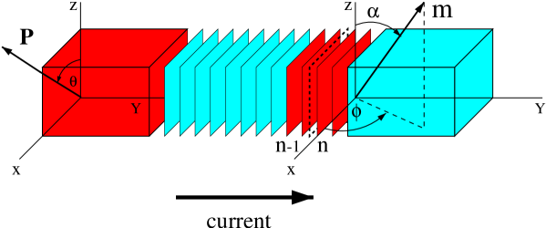
Figure 1: Schematic picture of a magnetic layer structure for current-induced switching (magnetic layers are darker, non-magnetic layers lighter).

The pinning of the magnetisation of the polarising magnet can be due to its large coercivity (thick magnet) or a strong uniaxial anisotropy. The role of the polarising magnet is to produce a stream of spin-polarised electrons, i.e. spin current, that is going to exert a torque on the magnetisation of the switching magnet whose magnetisation lies in the general direction of a unit vector ${\bf m}$. The orientation of the vector ${\bf m}$ is defined by the polar angles $\alpha$, $\phi$ shown in Fig. 1. There is a non-magnetic metallic layer inserted between the two magnets whose role is merely to separate magnetically the two magnetic layers and allow a strong charge current to pass. The total thickness of the whole trilayer sandwiched between two non-magnetic leads must be smaller than the spin diffusion length $l_{\rm sf}$ so that there are no spin flips due to impurities or spin-orbit coupling. A typical junction in which current-induced switching is studied experimentally albert is shown schematically in Fig. 2. The thickness of the polarising magnet is 40nm, that of the switching magnet 2.5nm and the non-magnetic spacer is 6nm thick. The materials for the two magnets and the spacer are cobalt and copper, respectively, which are those most commonly used. The junction cross section is oval-shaped with dimensions 60nm$\times$130nm. A small diameter is necessary so that the torque due to the Oersted field generated by a charge current of $10^{7}$-$10^{8}$ A/cm², required for current-induced switching, is much smaller than the spin-transfer torque we are interested in.

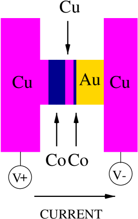
Figure 2: Schematic picture of a junction in which current-induced switching is studied experimentally.

The aim of most experiments is to determine the orientation of the switching magnet moment as a function of the current (applied bias) in the junction. Sudden jumps of the magnetisation direction, i.e. current-induced switching, are of particular interest. The orientation of the switching magnet moment ${\bf m}$ relative to that of the polarising magnet ${\bf p}$, which is fixed, is determined by measuring the resistance of the junction. Because of the GMR effect, the resistance of the junction is higher when the magnetisations of the two magnets are anti-parallel than when they are parallel, In other words, what is observed are hysteresis loops of resistance versus current. A typical experimental hysteresis loop of this type 16 is reproduced in Fig. 3.

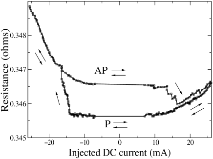
Figure 3: Resistance vs current hysteresis loop (after Grollier et al. 16 ).

It can be seen from Fig. 3 that, for any given current, the switching magnet moment is stationary (the junction resistance has a well defined value), i.e. the system is in a steady state. This holds everywhere on the hysteresis loop except for the two discontinuities where current-induced switching occurs. As indicated by the arrows jumps from the parallel (P) to anti-parallel (AP) configurations of the magnetisation, and from AP to P configurations, occur at different currents. It follows that in order to interpret experiments which exhibit such hysteresis behaviour, the first task of the theory is to determine from the LLG equation all the possible states and then investigate their dynamical stability. At the point of instability the system seeks out a new steady state, i.e. a discontinuous transition to a new steady state with the switched magnetisation occurs. We have tacitly assumed that there is always a steady state available for the system to jump to. There is now experimental evidence that this is not always the case. In the absence of any stable steady state the switching magnet moment remains permanently in the time-dependent state. This interesting case is implicit in the phenomenological LLG treatment and we shall discuss it in detail later.

In describing the switching magnet by a unique unit vector ${\bf m}$, we assume that it remains uniformly magnetised during the switching process. This is only strictly true when the exchange stiffness of the switching magnet is infinitely large. It is generally a good approximation as long as the switching magnet is small enough to remain single domain, so that the switching occurs purely by rotation of the magnetisation as in the Stoner-Wohlfarth theory 17 of field switching. This seems to be the case in many experiments albert ; 16 ; 18 ; 19

Before we can apply the LLG equation to study the time evolution of the unit vector ${\bf m}$ in the direction of the magnetisation of the switching magnet, we need to determine all the contributions to the torque acting on the switching magnet. Firstly, there is the spin-transfer torque ${\bf T}^{\rm s-t}$ which we discussed in Section II. Secondly, there is a torque due to the uniaxial in-plane and easy plane (shape) anisotropies. The easy-plane shape anisotropy torque arises because the switching magnet is a thin layer typically only a few nanometers thick. The in-plane uniaxial anisotropy is usually also a shape anisotropy arising from an elongated cross section of the switching magnet albert . We take the uniaxial anisotropy axis of the switching magnet to be parallel to the $z$-axis of the coordinate system shown in Fig. 1. Since the switching magnet lies in the $xz$-plane, we can write the total anisotropy field as

$${\bf H}_{\rm A}={\bf H}_{\rm u}+{\bf H}_{\rm p}$$ (18)

where ${\bf H}_{\rm u}$ and ${\bf H}_{\rm p}$ are given by

$${\bf H}_{\rm u}=H_{\rm u0}({\bf m}\cdot{\bf e}_{z}){\bf e}_{z},$$ (19)

$${\bf H}_{\rm p}=-H_{\rm p0}({\bf m}\cdot{\bf e}_{y}){\bf e}_{y}.$$ (20)

Here ${\bf e}_{x}$, ${\bf e}_{y}$ and ${\bf e}_{z}$ are unit vectors in the directions of the axes shown in Fig. 1. If we write the energy of the switching magnet in the anisotropy field as $-{\bf H}_{\rm A}\cdot\langle{\bf S}_{\rm tot}\rangle$, where $\langle{\bf S}_{\rm tot}\rangle$ is the total spin angular momentum of the switching magnet, them $H_{\rm u0}$,$H_{\rm p0}$ which measure the strengths of the uniaxial and easy-plane anisotropies have dimensions of frequency. These quantities may be converted to a field in tesla by multiplying by $\hbar/2\mu_{\rm B}=5.69\times 10^{-12}$.

We are now ready to study the time evolution of the unit vector ${\bf m}$ in the direction of the switching magnet moment. The LLG equation takes the usual form

$$\frac{{\rm d}{\bf m}}{{\rm d}t}+\gamma{\bf m}\times\frac{{\rm d}{\bf m}}{{\rm d}t}={\bm{\Gamma}}$$ (21)

where the reduced total torque ${\bm{\Gamma}}$ acting on the switching magnet is given by

$${\bm{\Gamma}}=\left[-\left({\bf H}_{\rm A}+{\bf H}_{\rm ext}\right)\times\langle{\bf S}_{\rm tot}\rangle+{\bf T}_{\perp}+{\bf T}_{\parallel}\right]/\left|\langle{\bf S}_{\rm tot}\rangle\right|.$$ (22)

Here ${\bf H}_{\rm ext}$ is an external field, in the same frequency units as ${\bf H}_{\rm A}$, and $\gamma$ is the Gilbert damping parameter. Following Sun sun , Eq. (21) may be written more conveniently as

$$\left(1+\gamma^{2}\right)\frac{{\rm d}{\bf m}}{{\rm d}t}={\bm{\Gamma}}-\gamma{\bf m}\times{\bm{\Gamma}}.$$ (23)

It is also useful to measure the strengths of all the torques in units of the strength of the uniaxial anisotropy sun . We shall, therefore, write the total reduced torque ${\bm{\Gamma}}$ in the form

$${\bm{\Gamma}}=H_{uo}\left\{({\bf m}\cdot{\bf e}_{z}){\bf m}\times{\bf e}_{z}-h_{\rm p}({\bf m}\cdot{\bf e}_{y}){\bf m}\times{\bf e}_{y}+v_{\parallel}(\psi){\bf m}\times({\bf p}\times{\bf m})+\left[v_{\perp}(\psi)+h_{\rm ext}\right]{\bf m}\times{\bf p}\right\}$$ (24)

where the relative strength of the easy plane anisotropy $h_{\rm p}=H_{\rm p0}/H_{\rm u0}$ and $v_{\parallel}(\psi)=vg_{\parallel}(\psi)$, $v_{\perp}(\psi)=vg_{\perp}(\psi)$ measure the strengths of the torques ${\bf T}_{\parallel}$ and ${\bf T}_{\perp}$. The reduced bias is defined by $v=eV_{\rm b}/(|\langle{\bf S}_{\rm tot}\rangle|H_{\rm u0})$ and has the opposite sign from the bias voltage since $e$ is negative. Thus positive $v$ implies a flow of electrons from the polarising to the switching magnet. The last contribution to the torque in Eq. (24) is due to the external field $H_{\rm ext}$ with $h_{\rm ext}=H_{\rm ext}/H_{\rm u0}$. The external field is taken in the direction of the magnetisation of the polarising magnet, as is the case in most experimental situations.

It follows from Eq. (21) that in a steady state ${\bm{\Gamma}}=0$. We shall first consider some cases of experimental importance where the steady state solutions are trivial and the important physics is concerned entirely with their stability. To discuss stability, we linearise Eq. (23), using Eq. (24), about a steady state solution ${\bf m}={\bf m}_{0}$. Thus

$${\bf m}={\bf m}_{0}+\xi{\bf e}_{\alpha}+\eta{\bf e}_{\phi},$$ (25)

where ${\bf e}_{\alpha}$, ${\bf e}_{\phi}$ are unit vectors in the direction ${\bf m}$ moves when $\alpha$ and $\phi$ are increased independently. The linearised equation may be written in the form

$$\frac{{\rm d}\xi}{{\rm d}\tau}=A\xi+B\eta;\quad\frac{{\rm d}\eta}{{\rm d}\tau}=C\xi+D\eta.$$ (26)

Following Sun sun , we have introduced the natural dimensionless time variable $\tau=tH_{\rm u0}/(1+\gamma^{2})$. The conditions for the steady state to be stable are

$$F=A+D\leqslant 0;\quad G=AD-BC\geqslant 0$$ (27)

excluding $F=G=0$ 20 . For simplicity we give these conditions explicitly only for the case where either $v_{\parallel}^{\prime}(\psi_{0})=v_{\perp}^{\prime}(\psi_{0})=0$, with $\psi_{0}=\cos^{-1}({\bf p}\cdot{\bf m}_{0})$, or ${\bf m}_{0}=\pm{\bf p}$. The case ${\bf m}_{0}=\pm{\bf p}$ is very common experimentally as is discussed below. The stability condition $G\geqslant 0$ may be written

$$Q^{2}v_{\parallel}^{2}+(Qh+\cos 2\alpha_{0})(Qh+\cos^{2}\alpha_{0})+h_{\rm p}\left\{Qh(1-3\sin^{2}\phi_{0}\sin^{2}\alpha_{0})+\cos 2\alpha_{0}(1-2\sin^{2}\alpha_{0}\sin^{2}\phi_{0})\right\}-$$

$$h_{\rm p}^{2}\sin^{2}\alpha_{0}\sin^{2}\phi_{0}(1-2\sin^{2}\phi_{0}\sin^{2}\alpha_{0})\geqslant 0,$$ (28)

where $v_{\parallel}=v_{\parallel}(\psi_{0})$, $h=v_{\perp}(\psi_{0})+h_{\rm ext}$ and $Q=\cos\psi_{0}$. The condition $F\leqslant 0$ takes the form

$$-2(v_{\parallel}+\gamma h)Q-\gamma(\cos 2\alpha_{0}+\cos^{2}\alpha_{0})-\gamma h_{\rm p}(1-3\sin^{2}\phi_{0}\sin^{2}\alpha_{0})\leqslant 0.$$ (29)

We now discuss several interesting examples, the first of these relating to experiments of Grollier et al. 18 and others. In these experiments the magnetisation of the polarising magnet, the uniaxial anisotropy axis and the external field are all collinear (along the in-plane $z$-axis in our convention). In this case the equation ${\bm{\Gamma}}=0$, with ${\bm{\Gamma}}$ given by Eq. (24), shows immediately that possible steady states are given by ${\bf m}_{0}=\pm{\bf p}(\alpha_{0}=0,\pi)$, corresponding to the switching magnet moment along the $z$-axis. These are the only solutions when $h_{\rm p}=0$. For $h_{\rm p}\neq 0$ other steady-state solutions may exist but in the parameter regime which has been investigated they are always unstable 13 . We shall assume this is always the case and concentrate on the solutions ${\bf m}_{0}=\pm{\bf p}$. In the state of parallel magnetisation (P) ${\bf m}_{0}={\bf p}$ we have $v_{\parallel}=vg_{\parallel}(0)$, $h=vg_{\perp}(0)+h_{\rm ext}$, $\alpha_{0}=0$ and $Q=1$. The stability conditions (III) and (29) become

$$\left[g_{\parallel}(0)\right]^{2}v^{2}+(vg_{\perp}(0)+h_{\rm ext}+1)^{2}+h_{\rm p}\left[vg_{\perp}(0)+h_{\rm ext}+1\right]\geqslant 0$$ (30)

$$g_{\parallel}(0)v+\gamma\left[vg_{\perp}(0)+h_{\rm ext}+1+\frac{1}{2}h_{\rm p}\right]\geqslant 0.$$ (31)

In the state of anti-parallel magnetisation (AP) ${\bf m}_{0}=-{\bf p}$ we have $v_{\parallel}=vg_{\parallel}(\pi)$, $h=vg_{\perp}(\pi)+h_{\rm ext}$, $\alpha_{0}=\pi$ and $Q=-1$. The stability conditions for the AP state are thus

$$\left[g_{\parallel}(\pi)\right]^{2}v^{2}+(-vg_{\perp}(\pi)-h_{\rm ext}+1)^{2}+h_{\rm p}\left[-vg_{\perp}(\pi)-h_{\rm ext}+1\right]\geqslant 0$$ (32)

$$g_{\parallel}(\pi)v+\gamma\left[vg_{\perp}(\pi)+h_{\rm ext}-1-\frac{1}{2}h_{\rm p}\right]\leqslant 0.$$ (33)

In the regime of low external field ($h_{\rm ext}\approx 1$, i.e. $H_{\rm ext}\approx H_{u0}$) we have $H_{\rm p}>>H_{\rm ext}$ ($h_{\rm p}\approx 100$). Eqs. (30) and (32) may be then approximated by

$$vg_{\perp}(0)+h_{\rm ext}+1>0$$ (34)

$$vg_{\perp}(\pi)+h_{\rm ext}-1<0.$$ (35)

Equation (34) corresponds to P stability and (35) to AP stability. It is convenient to define scalar quantities $T_{\perp}$, $T_{\parallel}$ by $T_{\perp}=g_{\perp}(\psi)\sin\psi$, $T_{\parallel}=g_{\parallel}(\psi)\sin\psi$, these being scalar components of spin-transfer torque in units of $eV_{\rm b}$ (cf. Eq. (II)). Then $g_{i}(0)=[{\rm d}T_{i}/{\rm d}\psi]_{\psi=0}$ and $g_{i}(\pi)=-[{\rm d}T_{i}/{\rm d}\psi]_{\psi=\pi}$ with $i=\perp,\parallel$. Model calculations 13 show that both $g_{\perp}$ and $g_{\parallel}$ can be of either sign, although positive values are more common. Also there is no general rule about the relative magnitude of $g_{i}(0)$ and $g_{i}(\pi)$.

We now illustrate the consequences of the above stability conditions by considering two limiting cases. We first consider the case $g_{\perp}(\psi)=0$, $g_{\parallel}>0$, as assumed by Grollier et. al 18 in the analysis of their data. In Fig. 4 we plot the regions of P and AP stability deduced from Eqs. (31),(33)-(35), in the ($v$,$h_{\rm ext}$)-plane. Grollier et al. plot current instead of bias but this should not change the form of the figure. Theirs is rather more complicated, owing to a less transparent stability analysis with unnecessary approximation. The only approximations made above, to obtain Eqs. (34) and(35), can easily be removed, which results in the critical field lines $h_{\rm ext}=\pm 1$ acquiring a very slight curvature given by $h_{\rm ext}\approx 1+[vg_{\parallel}(\pi)]^{2}/h_{\rm p}$ and $h_{\rm ext}\approx-1-[vg_{\parallel}(0)]^{2}/h_{\rm p}$. The critical biases in the figure are give by

$$v_{{\rm AP}\rightarrow{\rm P}} = \gamma\left[1+\frac{1}{2}h_{\rm p}-h_{\rm ext}\right]/g_{\parallel}(\pi)$$

$$v_{{\rm P}\rightarrow{\rm AP}} = -\gamma\left[1+\frac{1}{2}h_{\rm p}+h_{\rm ext}\right]/g_{\parallel}(0).$$ (36)

A downward slope from left to right of the corresponding lines in Fig. 4 is not shown there. Since the damping parameter $\gamma$ is small ($\gamma\approx 0.01$) this downward slope of the critical bias lines is also small. From Fig. 4 we can deduce the behaviour of resistance versus bias in the external field regimes $|h_{\rm ext}|<1$ and $|h_{\rm ext}|>1$.

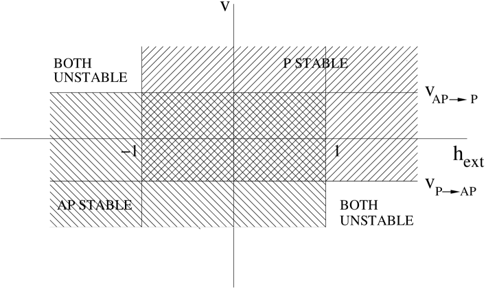
Figure 4: Bias-field stability diagram for $g_{\perp}(\psi)=0$, $g_{\parallel}(\psi)>0$. A small downward slope of the lines $V_{{\rm AP}\rightarrow{\rm P}}$,$V_{{\rm P}\rightarrow{\rm AP}}$ (see Eq. (III)) is not shown.

Consider first the case $|h_{\rm ext}|<1$. Suppose we start in the AP state with a bias $v=0$ which is gradually increased to $v_{{\rm AP}\rightarrow P}$. At this point the AP state becomes unstable and the system switches to the P state as $v$ increases further. On reducing $v$ the hysteresis loop is completed via a switch back to the AP state at the negative bias $v_{{\rm P}\rightarrow AP}$. The hysteresis loop is shown in Fig. 5(a). The increase in resistance R between the P and AP states is the same as would be produced by varying the applied field in a GMR experiment.

Figure 5: (a) Hysteresis loop of resistance vs bias for $|h_{\rm ext}|<1$; (b) Reversible behaviour (no hysteresis) for $|h_{\rm ext}|<-1$ (upper curve) and $h_{\rm ext}>1$ (lower curve). The dashed lines represent hypothetical behaviour of average resistance in regions of Fig. 4 marked “both unstable” where no steady states exist.

Now consider the case $h_{\rm ext}<-1$. Starting again in the AP state at $v=0$ we see from Fig. 4 that, on increasing $v$ to $v_{{\rm AP}\rightarrow{\rm P}}$, the AP state becomes unstable but there is no stable P state to switch to. This point is marked by an asterisk in Fig. 5(b). For $v>v_{{\rm AP}\rightarrow{\rm P}}$, the moment of the switching magnet is in a persistently time-dependent state. However, if $v$ is now decreased below $v_{{\rm P}\rightarrow{\rm AP}}$ the system homes in on the stable AP state and the overall behaviour is reversible, i.e. no switching and no hysteresis occur. When $h_{\rm ext}>1$ similar behaviour, now involving the P state, occurs at negative bias, as shown in Fig. 5(b). The dashed curves in Fig. 5(b) show a hypothetical time-averaged resistance in the regions of time-dependent magnetisation. As discussed later time-resolved measurements of resistance suggest that several different types of dynamics can occur in these regions.

It is clear from Fig. 5(a) that the jump AP$\rightarrow$P always occurs for positive bias $v$, which corresponds to flow of electrons from the polarising to the switching magnet. This result depends on the assumption that $g_{\parallel}>0$; if $g_{\parallel}<0$ it is easy to see that the sense of the hysteresis loop is reversed and the jump P$\rightarrow$AP occurs for positive $v$. To our knowledge this reverse jump has never been observed, although $g_{\parallel}<0$ can occur in principle and is predicted theoretically 13 for the Co/Cu/Co(111) system with a switching magnet consisting of a single atomic plane of Co. It follows from Eq. (III) that $|v_{{\rm P}\rightarrow{\rm AP}}/v_{{\rm AP}\rightarrow{\rm P}}|=|g_{\parallel}(\pi)/g_{\parallel}(0)|$ in zero external field. Experimentally this ratio, essentially the same as the ratio of critical currents, may be considerably less than 1 (e.g. $<0.5$ albert ), greater than 1 (e.g. $\approx 2$ 19 ) or close to 1 16 . Usually the field dependence of the critical current is found to be stronger than that predicted by Eq. (III) albert ; 16 .

We now discuss the reversible behaviour shown in Fig. 5(b) which occurs for $|h_{\rm ext}|>1$. The transition from hysteretic to reversible behaviour at a critical external field seems to have been first seen in pillar structures by Katine et al. 21 . Curves similar to the lower one in Fig. 5(b) are reported with $|v_{{\rm P}\rightarrow{\rm AP}}|$ increasing with increasing $h_{\rm ext}$, as expected from Eq. (III). Plots of the differential resistance ${\rm d}V/{\rm d}I$ show a peak near the point of maximum gradient of the dashed curve. Similar behaviour has been reported by several groups 22 ; 23 ; 24 . It is particularly clear in the work of Kiselev at al. 22 that the transition from hysteretic behaviour (as in Fig. 5(a)) to reversible behaviour with peaks in ${\rm d}V/{\rm d}I$ occurs at the coercive field 600 Oe of the switching layer ($h_{\rm ext}=1$). The important point about the peaks in ${\rm d}V/{\rm d}I$ is that for a given sign of $h_{\rm ext}$ they only occur for one sign of the bias. This clearly shows that this effect is due to spin-transfer and not to Oersted fields. Myers et al. 25 show a current-field stability diagram similar to the bias-field one of Fig. 4 with a critical field of 1500 Oe. They examine the time dependence of the resistance at room temperature with the field and current adjusted so that the system is in the “both unstable” region in the fourth quadrant of Fig. 4 but very close to its top left-hand corner. They observe telegraph-noise-type switching between approximately P and AP states with slow switching times in the range 0.1-10 s. Similar telegraph noise with faster switching times was observed by Urazhdin et al. 23 at current and field close to a peak in ${\rm d}V/{\rm d}I$. In the region of P and AP instability Kiselev et al. 22 and Pufall et al. 24 report various types of dynamics of precessional type and random telegraph switching type in the microwave Ghz regime. Kiselev et al. 22 propose that systems of the sort considered here might serve as nanoscale microwave sources or oscillators, tunable by current and field over a wide frequency range.

We now return to the stability conditions (31),(33)-(35) and consider the case of $g_{\perp}(\psi)\neq 0$ but $h_{\rm ext}=0$. These conditions of stability of the P state may be written approximately, remembering that $\gamma<<1$, $h_{\rm p}>>1$, as

$$vg_{\perp}(0)>-1,\quad vg_{\parallel}(0)>-\frac{1}{2}\gamma h_{\rm p}.$$ (37)

The conditions for stability of the AP state are

$$vg_{\perp}(\pi)<1,\quad vg_{\parallel}(\pi)<\frac{1}{2}\gamma h_{\rm p}.$$ (38)

In Fig. 6 we plot the regions of P and AP stability, assuming $g_{\perp}(0)=g_{\perp}(\pi)=g_{\perp}$ and $g_{\parallel}(0)=g_{\parallel}(\pi)=g_{\parallel}$ for simplicity. We also put $r=g_{\perp}/g_{\parallel}$.

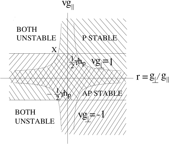
Figure 6: Stability diagram for $h_{\rm ext}=0$.

For $r>0$ we find the normal hysteresis loop as in Fig. 5(a) if we plot $R$ against $vg_{\parallel}$ (valid for either sign of $g_{\parallel}$). In Fig. 7 we plot the hysteresis loops for the cases $r_{\rm c}<r<0$ and $r<r_{\rm c}$, where $r_{\rm c}=-2/(\gamma h_{\rm p})$ is the value of $r$ at the point $X$ in Fig. 6.

Figure 7: Hysteresis loop for (a) $r_{\rm c}<r<0$; (b) $r<r_{\rm c}$.

The points labelled by asterisks have the same significance as in Fig. 5(b). If in Fig. 7(a) we increase $vg_{\parallel}$ beyond its value indicated by the right-hand asterisk we move into the “both-unstable” region where the magnetisation direction of the switching magnet is perpetually in a time-dependent state. Thus negative $r$ introduces behaviour in zero applied field which is similar to that found when the applied field exceeds the coercive field of the switching magnet for $r=0$. This behaviour was predicted by Edwards et al. 13 , in particular for a Co/Cu/Co(111) system with the switching magnet consisting of a Co monolayer. Zimmler et al. 26 use methods similar to the ones described here to analyse their data on a Co/Cu/Co nanopillar and deduce that $g_{\parallel}>0$, $r=g_{\perp}/g_{\parallel}\approx-0.2$. It would be interesting to carry out time-resolved resistance measurements on this system at large current density (corresponding to $vg_{\perp}<-1$) and zero external field.

So far we have considered the low-field regime ($H_{\rm ext}\approx$ coercive field of switching magnet) with both magnetisations and the external field in-plane. There is another class of experiments in which a high field, greater than the demagnetising field ($>2T$), is applied perpendicular to the plane of the layers. The magnetisation of the polarising magnet is then also perpendicular to the plane. This is the situation in the early experiments where a point contact was employed to inject high current densities into magnetic multilayers 27 ; 28 ; 29 . In this high-field regime a peak in the differential resistance ${\rm d}V/{\rm d}I$ at a critical current was interpreted as the onset of current-induced excitation of spin waves in which the spin-transfer torque leads to uniform precession of the magnetisation 6 ; 27 ; 28 . No hysteretic magnetisation reversal was observed and it seemed that the effect of spin-polarised current on the magnetisation is quite different in the low- and high-field regimes. Recently, however, Özyilmaz et al. 30 have studied Co/Cu/Co nanopillars ($\approx 100$nm in diameter) at $T=4.2$K for large applied fields perpendicular to the layers. They observe hysteretic magnetisation reversal and interpret their results using the Landau-Lifshitz equation. We now give a similar discussion within the framework of this section.

Following Özyilmaz et al., we neglect the uniaxial anisotropy term in Eq. (24) for the reduced torque ${\bm{\Gamma}}$ while retaining $H_{u0}$ as a scalar factor. Hence

$${\bm{\Gamma}}=H_{u0}\left\{\left[h_{\rm ext}+v_{\perp}(\psi)-h_{\rm p}\cos\psi\right]{\bf m}\times{\bf p}+v_{\parallel}(\psi){\bf m}\times({\bf p}\times{\bf m})\right\}$$ (39)

where ${\bf p}$ is the unit vector perpendicular to the plane. When $v_{\parallel}(\psi)\neq 0$ the only possible steady-state solutions of ${\bm{\Gamma}}=0$ are ${\bf m}_{0}=\pm{\bf p}$. On linearizing Eq. 23 about ${\bf m}_{0}$ as before we find that the condition $G\geqslant 0$ is always satisfied. The second stability condition $F<0$ becomes

$$\left[v_{\parallel}(\psi_{0})+\gamma(v_{\perp}(\psi_{0})+h_{\rm ext}-h_{\rm p})\right]\cos\psi_{0}>0$$ (40)

where $\psi_{0}=\cos^{-1}({\bf m}_{0}\cdot{\bf p})$. Applying this to the P state ($\psi_{0}=0$) and the AP state ($\psi_{0}=\pi$) we obtain the conditions

$$v>\gamma(h_{\rm p}-h_{\rm ext})/g(0)$$ (41)

$$v<-\gamma(h_{\rm p}+h_{\rm ext})/g(\pi),$$ (42)

where the first condition applies to the P stability and the second to the AP stability. Here $g(\psi)=g_{\parallel}(\psi)+\gamma g_{\perp}(\psi)$. The corresponding stability diagram is shown in Fig. 8, where we have assumed $g(\pi)>g(0)>0$ for definiteness.

Figure 8: Bias-field stability diagram for large external field ($h_{\rm ext}>h_{\rm p}$) perpendicular to the layers.

The boundary lines cross at $h_{\rm ext}=h_{\rm c}$, where $h_{\rm c}=h_{\rm p}[g(\pi)+g(0)]/[g(\pi)-g(0)]$. This analysis is only valid for fields larger than the demagnetising field ($h_{\rm ext}>h_{\rm p}$) and we see from the figure that for $h_{\rm ext}>h_{\rm c}$ hysteretic switching occurs. This takes place for only one sign of the bias (current) and the critical biases (currents) increase linearly with $h_{\rm ext}$ as does the width of the hysteresis loop $|v_{{\rm P}\rightarrow{\rm AP}}-v_{{\rm AP}\rightarrow{\rm P}}|$. This accords with the observations of Özyilmaz et al. The critical currents are not larger than those in the low-field or zero-field regimes (cf. Eqs. (41), (42) with Eq. (III)) and yet the magnetisation of the switching magnet can be switched against a very large external field. However, in this case the AP state is only stabilised by maintaining the current.

The experiments on spin transfer discussed above have mainly been carried out at constant temperature, typically $4.2$K or room temperature. The effect on current-driven switching of varying the temperature has recently been studied by several groups 23 ; 25 ; 31 . The standard Néel-Brown theory of thermal switching 32 does not apply because the Slonczewski in-plane torque is not derivable from an energy function. Li and Zhang 33 have generalised the standard stochastic Landau-Lifschitz equation, which includes white noise in the effective applied field, to include spin transfer torque. In this way they have successfully interpreted some of the experimental data. A full discussion of this work is outside the scope of the present review. However it should be pointed out that in addition to the classical effect of white noise there is an intrinsic temperature dependence of quantum origin. This arises from the Fermi distribution functions which appear in expressions for the spin-transfer torque (see Eqs. (14) and (12)).

So far we have discussed steady-state solutions of the LLG equation (23). It is important to study the magnetisation dynamics of the switching layer in the situation during the jumps AP$\rightarrow$P and P$\rightarrow$AP of the hysteresis curve in zero external field, and secondly under conditions where only time-dependent solutions are possible, for example in the regions of sufficiently strong current and external field marked ”both unstable” in Fig. 4. The first situation has been studied by Sun sun , assuming single-domain behaviour of the switching magnet, and by Miltat et al. 34 with more general micromagnetic configurations. Both situations have been considered by Li and Zhang 35 . In the second case they find precessional states, and the possibility of ”telegraph noise” at room temperature, as seen experimentally in Refs. 22 ; 24 . Switching times (AP$\rightarrow$P and P$\rightarrow$AP) are estimated to be of the order 1ns. Micromagnetic simulations 34 indicate that the Oersted field cannot be completely ignored for typical pillars with diameter of the order of 100nm.

Finally, in this section, we briefly discuss some practical considerations which may ultimately decide whether current-induced switching is useful in spintronics. Sharp switching, with nearly rectangular hysteresis loops, is obviously desirable and this demands single-domain behaviour. In experiments on nanopillars of circular cross section 21 multidomain behaviour was observed with the switching transition spread over a range of current. Subsequently the same group albert found sharp switching in pillars whose cross-section was an elongated hexagon, which introduces strong uniaxial in-plane shape anisotropy. It was known from earlier magnetisation studies of nanomagnet arrays 36 that such a shape anisotropy can result in single domain behaviour. A complex switching transition need not necessarily indicate multidomain behaviour. It could also arise from a marked departure of $T_{\perp}(\psi)$ and/or $T_{\parallel}(\psi)$ from sinusoidal behaviour, such as occurs near $\psi=\pi$ in calculations for Co/Cu/Co(111) with two atomic planes of Co in the switching magnet (see Fig. 9(b)). In the calculations of the corresponding hysteresis loops (Fig. 11) the torques were approximated by sine curves but an accurate treatment would certainly complicate the AP$\rightarrow$P transition which occurs at negative bias in Fig. 11(b). Studies of this effect are planned.

The critical current density for switching is clearly an important parameter. From Eq. (III) the critical reduced bias for the P$\rightarrow$AP transition is to a good approximation given by $-\gamma h_{\rm p}/[2g_{\parallel}(0)]$. Using the definitions of reduced quantities given after Eq. (24), we may write the actual critical bias in volts as

$$V_{P\rightarrow AP}=M\gamma M_{\rm s}H_{\rm d}/[2g_{\parallel}(0)|e|],$$ (43)

where $M$ is the number of atomic planes in the switching magnet, $M_{\rm s}$ is the average moment ($J/T$) of the switching magnet per atomic plane per unit area, and $H_{\rm d}=\hbar H_{\rm p0}/(2\mu_{\rm B})$ is the easy-plane anisotropy field in tesla. As expressed earlier $g_{\parallel}(0)=({\rm d}T_{\parallel}/{\rm d}\psi)_{\psi=0}$ where the torque $T_{\parallel}$ is per unit area in units of $eV_{\rm B}$. (The calculated torques in Figs. 9 and 10 of Sec. V are per surface atom so that if these are used to determine $g_{\parallel}(0)$ in Eq. (43) $M_{\rm s}$ must be taken per surface atom.)

An obvious way to reduce the critical bias, and hence the critical current, is to reduce $M$, the thickness of the switching magnet. Calculations show 13 (see also Fig. 10) that $g_{\parallel}$ does not decrease with $M$ and may, in fact, increase for small values such as $M=2$. Careful design of the device might also increase $g_{\parallel}(0)$ beyond the values ($<0.01$ per surface atom) which seem to be obtainable in simple trilayers 13 . Jiang et al. 37 ; 38 , have studied various structures in which the polarising magnet is pinned by an adjacent antiferromagnet (exchange biasing) and in which a thin Ru layer is incorporated between the switching layer and the lead. Critical current densities of $2\times 10^{6}$Acm^-2 have been obtained which are substantially lower than those in Co/Cu/Co trilayers. Such structures can quite easily be investigated theoretically by the methods of Section V.

Decreasing the magnetisation $M_{\rm s}$, and hence the demagnetising field ($\propto H_{\rm d}$), would be favourable but $g_{\parallel}$ then tends to decrease also 13 . A possible way of decreasing $H_{\rm d}$ without decreasing local magnetic moments in the system is to use a synthetic ferrimagnet as the switching magnet 39 . The Gilbert damping factor $\gamma$ is another crucial parameter but it is uncertain whether this can be decreased significantly. However, the work of Capelle and Gyorffy 40 is an interesting theoretical development. The search for structures with critical current densities low enough for use in spintronic devices ($10^{5}$Acm^-2 perhaps) 41 is an enterprise where experiment and quantitative calculations 13 should complement each other fruitfully.

IV Quantitative theory of spin-transfer torque

IV.1 General principles

To put the phenomenological treatment of Sec. III on a first-principle quantitative basis we must calculate the spin-transfer torques (Eqs. (II) in a steady state for real systems. For this purpose it is convenient to describe the magnetic and nonmagnetic layers of Fig. 1 by tight-binding models, in general multiorbital with s, p, and d orbitals whose one-electron parameters are fitted to first-principle bulk band structure 42 . The hamiltonian is therefore of the form

$$H=H_{0}+H_{\rm int}+H_{\rm anis}$$ (44)

where the one-electron hopping term $H_{0}$ is given by

$$H_{0}=\sum_{k_{\parallel}\sigma}\sum_{m\mu,n\nu}t_{m\mu,n\nu}({\bf k}_{\parallel})c^{\dagger}_{{\bf k}_{\parallel}m\mu\sigma}c_{{\bf k}_{\parallel}n\nu\sigma},$$ (45)

where $c^{\dagger}_{k_{\parallel}m\mu\sigma}$ creates an electron in a Bloch state, with in-plane wave vector ${\bf k}_{\parallel}$ and spin $\sigma$, formed from a given atomic orbital $\mu$ in plane $m$. Eq. 45 generalises the single orbital eq. (1). $H_{\rm int}$ is an on-site interaction between electrons in d orbitals which leads to an exchange splitting of the bands in the ferromagnets and is neglected in the spacer and lead. Finally, $H_{\rm anis}$ contains anisotropy fields in the switching magnet and is given by

$$H_{\rm anis}=-\sum_{n}{\bf S}_{n}\cdot{\bf H}_{\rm A},$$ (46)

where ${\bf S}_{n}$ is the operator of the total spin angular momentum of plane $n$ and ${\bf H}_{\rm A}$ is given by Eqs. (18)-(20) with the unit vector ${\bf m}$ in the direction of $\sum_{n}\langle{\bf S}_{n}\rangle$, where $\langle{\bf S}_{n}\rangle$ is the thermal average of ${\bf S}_{n}$. We assume here that the anisotropy fields $H_{\rm u0}$,$H_{\rm p}$ are uniform throughout the switching magnet but we could generalise to include, for example, a surface anisotropy.

In the tight-binding description, the spin angular momentum operator ${\bf S}_{n}$ is given by

$${\bf S}_{n}=\frac{1}{2}\hbar\sum_{k_{\parallel\mu}}(c^{\dagger}_{k_{\parallel}n\mu\uparrow},c^{\dagger}_{k_{\parallel}n\mu\downarrow}){\bm{\sigma}}(c_{k_{\parallel}n\mu\uparrow},c_{k_{\parallel}n\mu\downarrow})^{\rm T}$$ (47)

and the corresponding operator for the spin angular momentum current between planes $n-1$ and $n$ is

$${\bf j}_{n-1}=-\frac{1}{2}\hbar\sum_{{\bf k}_{\parallel}\mu\nu}t({\bf k}_{\parallel})_{n\nu,n-1\mu}\left(c^{\dagger}_{k_{\parallel}n\nu\uparrow},c^{\dagger}_{k_{\parallel}n\nu\downarrow}\right){\bm{\sigma}}\left(c_{k_{\parallel}n-1\mu\uparrow},c_{k_{\parallel}n-1\mu\downarrow}\right)^{\rm T}+{\rm h.c.},$$ (48)

which generalises the single orbital expression (2). The rate of change of ${\bf S}_{n}$ in the switching magnet is given by

$${\rm i}\hbar\frac{{\rm d}{\bf S}_{n}}{{\rm d}t}=[{\bf S}_{n},H_{0}]+[{\bf S}_{n},H_{\rm anis}].$$ (49)

This results holds since the spin operator commutes with the interaction hamiltonian $H_{\rm int}$.

It is straightforward to show that

$$[{\bf S}_{n},H_{0}]={\rm i}\hbar({\bf j}_{n-1}-{\bf j}_{n}),$$ (50)

and

$$[{\bf S}_{n},H_{\rm anis}]=-{\rm i}\hbar({\bf H}_{\rm A}\times{\bf S}_{n}).$$ (51)

On taking the thermal average, Eq. (49) becomes

$$\langle\frac{{\rm d}{\bf S}_{n}}{{\rm d}t}\rangle=\langle{\bf j}_{n-1}\rangle-\langle{\bf j}_{n}\rangle-{\bf H}_{\rm A}\times\langle{\bf S}_{\rm tot}\rangle,$$ (52)

This corresponds to an equation of continuity, stating that the rate of change of spin angular momentum on plane $n$ is equal to the difference between the rate of flow of this quantity onto and off the plane, plus the rate of change due to precession around the field ${\bf H}_{\rm A}$. When Eq. (52) is summed over all planes in the switching magnet we have

$$\frac{{\rm d}}{{\rm d}t}\langle{\bf S}_{\rm tot}\rangle={\bf T}^{\rm s-t}-{\bf H}_{\rm A}\times\langle{\bf S}_{\rm tot}\rangle,$$ (53)

where the total spin-transfer torque ${\bf T}^{\rm s-t}$ is given by Eq. (14) and $\langle{\bf S}_{\rm tot}\rangle$ is the total spin angular momentum of the switching magnet. Equation (53) is equivalent to Eq. (21), for zero external field, in the absence of damping. Equation (14) shows how ${\bf T}^{\rm s-t}$ required for the phenomenological treatment of Sec. III is to be determined from the calculated spin currents in the spacer and lead. As discussed in Sec. III, the magnetization of a single-domain sample is essentially uniform and the spin-transfer torque ${\bf T}^{\rm s-t}$ depends on the angle $\psi$ between the magnetisations of the polarising and switching magnets.

To consider time-dependent solutions of Eq. (21) it is necessary to calculate ${\bf T}^{\rm s-t}$ for arbitrary angle $\psi$ and for this purpose ${\bf H}_{\rm A}$ can be neglected. To reduce the calculation of the spin-transfer torque to effectively a one-electron problem, we replace $H_{\rm int}$ by a selfconsistent exchange field term $-\sum_{n}{\bf S}_{n}\cdot{\bm{\Delta}}_{n}$, where the exchange field ${\bm{\Delta}}_{n}$ should be determined selfconsistently in the spirit of an unrestricted Hartree-Fock (HF) or local spin density (LSD), approximation. The essential selfconsistency condition in any HF or LSD calculation is that the local moment $\langle{\bf S}_{n}\rangle$ in a steady state is in the same direction as ${\bm{\Delta}}_{n}$. Thus we require

$${\bm{\Delta}}_{n}\times\langle{\bf S}_{n}\rangle=0$$ (54)

for each atomic plane of the switching magnet. It is useful to consider first the situation when there is no applied bias and the polarising and switching magnets are separated by a spacer which is so thick that the zero-bias oscillatory exchange coupling 44 is negligible. In that case we have two independent magnets and the selfconsistent exchange field in every atomic plane of the switching magnet is parallel to its total magnetisation which is uniform and assumed to be along the $z$-axis. Referring to Fig. 1 the selfconsistent solution therefore corresponds to uniform exchange fields in the polarising and switching magnets which are at an assumed angle $\psi=\theta$ with respect to one another.

When a bias $V_{\rm b}$ is applied , with a uniform exchange field ${\bm{\Delta}}=\Delta{\bf e}_{z}$ in the switching magnet imposed, the calculated local moments $\langle{\bf S}_{n}\rangle$ will deviate from the $z$-direction so that the solution is not selfconsistent. To prepare a selfconsistent state with ${\bm{\Delta}}$ and all $\langle{\bf S}_{n}\rangle=\langle{\bf S}\rangle$ in the $z$-direction it is necessary to apply fictitious constraining fields ${\bf H}_{n}$ of magnitude proportional to $V_{\rm b}$. The local field for plane $n$ is thus ${\bm{\Delta}}+{\bf H}_{n}$ but to calculate the spin currents in the spacer and lead, and hence ${\bf T}^{\rm s-t}$ from Eq. (14), the fields ${\bf H}_{n}$, of the order of $V_{\rm b}$, may be neglected compared with ${\bf\Delta}$. Although the fictitious constraining fields ${\bf H}_{n}$ need therefore never be calculated, it is interesting to see that they are in fact related to ${\bf T}^{\rm s-t}$. For the constrained self-consistent steady state ($\langle{\bf S}_{n}\rangle=\langle{\bf S}\rangle$, $\langle{\bf\dot{S}}_{n}\rangle=0$) in the presence of the constraining fields, with ${\bf H}_{\rm A}$ neglected as discussed above, it follows from Eq. (52) that

$$\langle{\bf j}_{\bf n-1}\rangle-\langle{\bf j}_{\bf n}\rangle=(\Delta+{\bf H}_{n})\times\langle S\rangle={\bf H}_{n}\times\langle{\bf S}\rangle,$$ (55)

where the local field ${\bm{\Delta}}+{\bf H}_{n}$ replaces ${\bf H}_{\rm A}$. On summing over all atomic planes $n$ in the switching magnet we have

$${\bf T}^{\rm s-t}=\langle{\bf j}_{\rm spacer}\rangle-\langle{\bf j}_{\rm lead}\rangle=\sum_{n}{\bf H}_{n}\times\langle{\bf S}\rangle.$$ (56)

Thus, as expected, in the prepared state with a given angle $\psi$ between the magnetisations of the magnetic layers the spin-transfer torque is balanced by the total torque due to the constraining fields.

In the simple model of Section II, with infinite exchange splitting in the magnets, the local moment is constrained to be in the direction of the exchange field so the question of selfconsistency is not raised.

The main conclusion of this Section is that the spin-transfer torque for a given angle $\psi$ between magnetisations may be calculated using uniform exchange fields making the same angle with one another. Such calculations are described in Sec. II and V. The use of this spin-transfer torque in the LLG equation of Section III completes what we shall call the ”standard model” (SM). It underlies the original work of Slonczewski 3 and most subsequent work. The spin-transfer torque calculated in this way should be appropriate even for time-dependent solutions of the LLG equation. This is based on the reasonable assumption that the time for the electronic system to attain a ”constrained steady state” with given $\psi$ is short compared with the time-scale ($\approx$1ns) of the macroscopic motion of the switching magnet moment.

Although the SM is a satisfactory way of calculating the spin-transfer torque its lack of selfconsistency leads to some non-physical concepts. The first of these is the ”transverse spin accumulation” in the switching magnet 46 ; 47 , This refers to the deviations of local moments $\langle{\bf S}_{n}\rangle$ from the direction of the exchange field, assumed uniform in the SM. In a self-consistent treatment such deviations do not occur because the exchange field is always in the direction of the local moment. A related non-physical concept is the ”spin decoherence length” over which the spin accumulation is supposed to decay 46 ; 47 , More detailed critiques of these concepts are given elsewhere 13 ; em .

IV.2 Keldysh formalism for fully realistic calculations of the spin-transfer torque

The wave-function approach to spin-transfer torque described in Section II is difficult to apply to realistic multiorbital systems. For this purpose Green functions are much more convenient and Keldysh 11 developed a Green function approach to the non-equilibrium problem of electron transport. In this section we apply this method to calculate spin currents in a magnetic layer structure, following Edwards et al. 13 .

The structure we consider is shown schematically in Fig. 1. It consists of a thick (semi-infinite) left magnetic layer (polarising magnet), a nonmagnetic metallic spacer layer of $N$ atomic planes, a thin switching magnet of $M$ atomic planes, and a semi-infinite lead. The broken line between the atomic planes $n-1$ and $n$ represents a cleavage plane separating the system into two independent parts so that charge carriers cannot move between the two surface planes $n-1$ and $n$. It will be seen that our ability to cleave the whole system in this way is essential for the implementation of the Keldysh formalism. This can be easily done with a tight-binding parametrisation of the band structure by simply switching off the matrix of hopping integrals $t_{n\nu,n-1\mu}$ between atomic orbitals $\nu$, $\mu$ localised in planes $n-1$ and $n$. We therefore adopt the tight-binding description with the Hamiltonian defined by Eqs. (44-47).

To use the Keldysh formalism 11 ; 12 ; 53 to calculate the charge or spin currents flowing between the planes $n-1$ and $n$, we consider an initial state at time $\tau=-\infty$ in which the hopping integral $t_{n\nu,n-1\mu}$ between planes $n-1$ and $n$ is switched off. Then both sides of the system are in equilibrium but with different chemical potentials $\mu_{\rm L}$ on the left and $\mu_{\rm R}$ on the right, where $\mu_{\rm L}-\mu_{\rm R}=eV_{\rm b}$. The interplane hopping is then turned on adiabatically and the system evolves to a steady state. The cleavage plane, across which the hopping is initially switched off, may be taken in either the spacer or in one of the magnets or in the lead. In principle, the Keldysh method is valid for arbitrary bias $V_{\rm b}$ but here we restrict ourselves to small bias corresponding to linear response. This is always reasonable for a metallic system. For larger bias, which might occur with a semiconductor or insulator as spacer, electrons would be injected into the right part of the system far above the Fermi level and many-body processes neglected here would be important. Following Keldysh 11 ; 12 , we define a two-time matrix

$$G_{\rm RL}^{+}(\tau,\tau^{\prime})={\rm i}\langle c_{\rm L}^{\dagger}(\tau^{\prime})c_{\rm R}(\tau)\rangle,$$ (57)

where $R\equiv(n,\nu,\sigma^{\prime})$ and $L\equiv(n-1,\mu,\sigma)$, and we suppress the $k_{\parallel}$ label. The thermal average in Eq. (57) is calculated for the steady state of the coupled system. The matrix $G_{\rm RL}^{\dagger}$ has dimensions $2m\times 2m$ where $m$ is the number of orbitals on each atomic site, and is written so that the $m\times m$ upper diagonal block contains matrix elements between $\uparrow$ spin orbitals and the $m\times m$ lower diagonal block relates to $\downarrow$ spin. $2m\times 2m$ hopping matrices $t_{\rm LR}$ and $t_{\rm RL}$ are written similarly and in this case only the diagonal blocks are nonzero. If we denote $t_{\rm LR}$ by $t$, then $t_{\rm RL}=t^{\dagger}$. We also generalise the definition of ${\bm{\sigma}}$ so that its components are now direct products of the $2\times 2$ Pauli matrices $\sigma_{x}$, $\sigma_{y}$, $\sigma_{z}$, and the $m\times m$ unit matrix. The thermal average of the spin current operator, given by Eq. (49), may now be expressed as

$$\langle{\bf j}_{n-1}\rangle=\frac{1}{2}\sum_{{\bf k}_{\parallel}}{\rm Tr}\left\{\left[G_{\rm RL}^{+}\left(\tau,\tau\right)t-G_{\rm LR}^{+}(\tau,\tau)t^{\dagger}\right]{\bm{\sigma}}\right\}.$$ (58)

Introducing the Fourier transform $G^{+}(\omega)$ of $G^{+}(\tau,\tau^{\prime})$ , which is a function of $\tau-\tau^{\prime}$, we have

$$\langle{\bf j}_{n-1}\rangle=\frac{1}{2}\sum_{{\bf k}_{\parallel}}\int\frac{{\rm d}\omega}{2\pi}{\rm Tr}\left\{\left[G_{\rm RL}^{+}\left(\omega\right)t-G_{\rm LR}^{+}(\omega)t^{\dagger}\right]{\bm{\sigma}}\right\}.$$ (59)

The charge current is given by Eq. (59) with $\frac{1}{2}{\bm{\sigma}}$ replaced by the unit matrix multiplied by $e/\hbar$.

Following Keldysh 11 ; 12 we now write

$$G_{\rm AB}^{+}(\omega)=\frac{1}{2}\left(F_{\rm AB}+G_{\rm AB}^{\rm a}-G_{\rm AB}^{\rm r}\right),$$ (60)

where the suffices $A$ and $B$ are either $R$ or $L$. $F_{\rm AB}(\omega)$ is the Fourier transform of

$$F_{\rm AB}(\tau,\tau^{\prime})=-{\rm i}\langle[c_{\rm A}(\tau),c_{\rm B}^{\dagger}(\tau^{\prime})]_{-}\rangle$$ (61)

and $G^{\rm a}$, $G^{\rm r}$ are the usual advanced and retarded Green functions 54 . Note that in 11 and 12 the definitions of $G^{\rm a}$ and $G^{\rm r}$ are interchanged and that in the Green function matrix defined by these authors $G^{+}$ and $G^{-}$ should be interchanged.

Charge and spin current are related by Eqs. (59) and (60) to the quantities $G^{\rm a}$, $G^{\rm r}$ and $F_{\rm AB}$. The latter are calculated for the coupled system by starting with decoupled left and right systems, each in equilibrium, and turning on the hopping between planes L and R as a perturbation. Hence, we express $G^{\rm a}$, $G^{\rm r}$ and $F_{\rm AB}$ in terms of retarded surface Green functions $g_{L}\equiv g_{\rm LL}$, $g_{\rm R}\equiv g_{\rm RR}$ for the decoupled equilibrium system. It is then found 13 that the spin current between the planes $n-1$ and $n$ can be written as the sum $\langle{\bf j}_{n-1}\rangle=\langle{\bf j}_{n-1}\rangle_{1}+\langle{\bf j}_{n-1}\rangle_{2}$, where the two contributions to the spin current $\langle{\bf j}_{n}\rangle_{1}$, $\langle{\bf j}_{n}\rangle_{2}$ are given by

$$\langle{\rm j}_{n-1}\rangle_{1}=\frac{1}{4\pi}\sum_{{\bf k}_{\parallel}}\int{\rm d}\omega\Re{\rm Tr}[(B-A){\bm{\sigma}}][f(\omega-\mu_{\rm L})+f(\omega-\mu_{\rm R})].$$ (62)

$$\langle{\rm j}_{n-1}\rangle_{2}=\frac{1}{2\pi}\sum_{{\bf k}_{\parallel}}\int{\rm d}\omega\Re{\rm Tr}\left\{[g_{\rm L}tABg_{\rm R}^{\dagger}t^{\dagger}-AB+\frac{1}{2}(A+B)]{\bm{\sigma}}\right\}[f(\omega-\mu_{\rm L})-f(\omega-\mu_{\rm R})].$$ (63)

Here, $A=[1-g_{\rm R}t^{\dagger}g_{\rm L}t]^{-1}$, $B=[1-g^{\dagger}_{\rm R}t^{\dagger}g^{\dagger}_{\rm L}t]^{-1}$, and as in Section II $f(\omega-\mu)$ is the Fermi function with chemical potential $\mu$ and $\mu_{\rm L}-\mu_{\rm R}=eV_{\rm b}$. In the linear-response case of small bias which we are considering, the Fermi functions in Eq. (63) are expanded to first order in $V_{\rm b}$. Hence the energy integral is avoided, being equivalent to multiplying the integrand by $eV_{\rm b}$ and evaluating it at the common zero-bias chemical potential $\mu_{0}$.

It can be seen that Eqs. (62) and (63), which determine the spin and the charge currents, depend on just two quantities, i.e. the surface retarded one-electron Green functions for a system cleaved between two neighbouring atomic planes. The surface Green functions can be determined without any approximations by the standard adlayer method (see e.g. 42 ; 44 ) for a fully realistic band structure.

We first note that there is a close correspondence between Eqs. (62), (63) and the generalised Landauer formula (12). The first term in Eq. (12) corresponds to the zero-bias spin current $\langle{\bf j}_{n-1}\rangle_{1}$ given by Eq. (62). When the cleavage plane is taken in the spacer, the spin current $\langle{\bf j}_{n-1}\rangle_{1}$ determines the oscillatory exchange coupling between the two magnets and it is easy to verify that the formula for the exchange coupling obtained from Eq. (62) is equivalent to the formula used in previous total energy calculations of this effect 42 ; 44 . The contribution to the transport spin current given by Eq. (63) clearly corresponds to the second term in the Landauer formula (12) which is proportional to the bias in the linear response limit. Placing the cleavage plane first between any two neighbouring atomic planes in the spacer and then between any two neighbouring planes in the lead, we obtain from Eq. (63) the total spin-transfer torque ${\bf T}^{\rm s-t}$ of Eq. (14) in Section II.

The equivalence of the Keldysh and Landauer methods has been demonstrated by calculating the currents (62) and (63) analytically for the simple single orbital model of Section II. The results of that section, such as Eq. (15) are reproduced 13 .

V Quantitative results for Co/Cu/Co(111)

We now discuss the application of the Keldysh formalism to a real system. In particular we consider a realistic multiorbital model of fcc Co/Cu/Co(111) with tight-binding parameters fitted to the results of the first-principles band structure calculations, as described previously 42 ; 44 .

Referring to Fig. 1, the system considered by Edwards et al. 13 consists of a semi-infinite slab of Co (polarising magnet), the spacer of 20 atomic planes of Cu, the switching magnet containing $M$ atomic planes of Co, and the lead which is semi-infinite Cu. The spacer thickness of 20 atomic planes of Cu was chosen so that the contribution of the oscillatory exchange coupling term is so small that it can be neglected. The spin currents in the right lead and in the spacer were determined from Eq. (63). Figure 9(a),(b) shows the angular dependences of $T_{\parallel}$, $T_{\perp}$ for the cases $M=1$ and $M=2$. respectively.

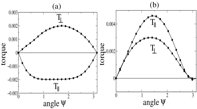
Figure 9: Dependence of the spin-transfer torque $T_{\parallel}$ and $T_{\perp}$ for Co/Cu/Co(111) on the angle $\psi$. The torques per surface atom are in units of $eV_{\rm b}$. Figure (a) is for $M=1$, and (b) for $M=2$ monolayers of Co in the switching magnet.

For the monolayer switching magnet, the torques $T_{\parallel}$ and $T_{\perp}$ are equal in magnitude and they have opposite sign. However, for $M=2$, the torques have the same sign and $T_{\perp}$ is somewhat smaller than $T_{\parallel}$. A negative sign of the ratio of the two torque components has important and unexpected consequences for hysteresis loops as already discussed in Section III. It can be seen that the angular dependence of both torque components is dominated by a $\sin\psi$ factor but distortions from this dependence are clearly visible. In particular, the slopes at $\psi=0$ and $\psi=\pi$ are quite different. As pointed out in Section III, this is important in the discussion of the stability of steady states and leads to quite different magnitudes of the critical biases $V_{\rm P}\rightarrow V_{\rm AP}$ and $V_{\rm AP}\rightarrow V_{\rm P}$.

In Fig. 10 we reproduce the dependence of $T_{\perp}$ and $T_{\parallel}$ on the thickness of the Co switching magnet. It can be seen that the out-of-plane torque $T_{\perp}$ becomes smaller than $T_{\parallel}$ for thicker switching magnets.

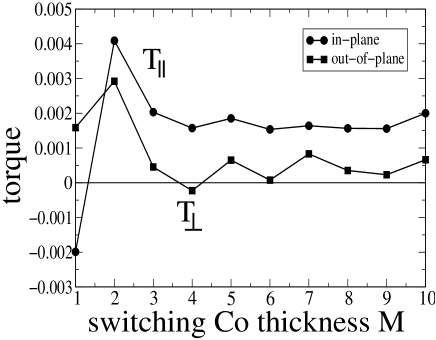
Figure 10: Dependence of the spin-transfer torque $T_{\parallel}$ and $T_{\perp}$ for Co/Cu/Co(111) on the thickness of the switching magnet $M$ for $\psi=\pi/3$. The torques are in units of $eV_{\rm b}$.

However, $T_{\perp}$ is by no means negligible (27$\%$ of $T_{\parallel}$) even for a typical experimental thickness of the switching Co layer of ten atomic planes. It is also interesting that beyond the monolayer thickness, the ratio of the two torques is positive with the exception of $M=4$.

The microscopically calculated spin-transfer torques for Co/Cu/Co(111) were used by Edwards et al. 13 as an input into the phenomenological LLG equation. For simplicity the torques as functions of $\psi$ were approximated by sine curves but this is not essential. The LLG equation was first solved numerically to determine all the steady states and then the stability discussion outlined in the phenomenological section was applied to determine the critical bias for which instabilities occur. Finally, the ballistic resistance of the structure was evaluated from the real-space Kubo formula at every point of the steady state path. Such a calculation for the realistic Co/Cu system then gives hysteresis loops of the resistance versus bias which can be compared with the observed hysteresis loops. The LLG equation was solved including a strong easy-plane anisotropy with $h_{\rm p}=100$. If we take $H_{\rm u0}=1.86\times 10^{9}$sec^-1, corresponding to a uniaxial anisotropy field of about 0.01T, this value of $h_{\rm p}$ corresponds to the shape anisotropy for a magnetisation of $1.6\times 10^{6}$A/m, similar to that of Co sun . Also a realistic value sun of the Gilbert damping parameter $\gamma=0.01$ was used. Finally, referring to the geometry of Fig. 1, two different values of the angle $\theta$ were employed in these calculations: $\theta=2$rad and $\theta=3$rad, the latter value being close to the value of $\pi$ which is realised in most experiments.

We first reproduce in Fig. 11 the hysteresis loops for the case of Co switching magnet consisting of two atomic planes. We note that the ratio $r=T_{\perp}/T_{\parallel}\approx 0.65$ deduced from Fig. 9 is positive in this case. Fig. 11(a) shows the hysteresis loop for $\theta=2$ and Fig. 11(b) that for $\theta=3$.

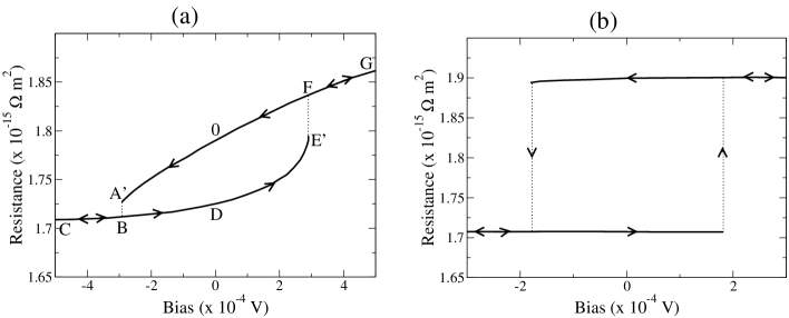
Figure 11: Resistance of the Co/Cu/Co(111) junction as a function of the applied bias, with $M=2$ monolayers of Co in the switching magnet. (a) is for $\theta=2$rad and (b) for $\theta=3$rad.

The hysteresis loop for $\theta=3$ shown in Fig. 11(b) is an illustration of the stability scenario in zero applied field with $r>0$ discussed in Section III. As pointed out there the hysteresis curve is that of Fig. 5(a) which agrees with Fig. 11(b) when we remember that the reduced bias used in Fig. 5 has the opposite sign from the bias in volts used in Fig. 11. It is rather interesting that the critical bias for switching is $\approx 0.2$mV both for $\theta=2$ and $\theta=3$. When this bias is converted to the current density using the calculated ballistic resistance of the junction, it is found 13 that the critical current for switching is $\approx 10^{7}$A/cm², which is in very good agreement with experiments albert .

The hysteresis loops for the case of the Co switching magnet consisting of a single atomic plane are reproduced in Fig. 12. The values of $h_{\rm p}$, $\gamma$, $H_{\rm u0}$, and $\theta$ are the same as in the previous example.

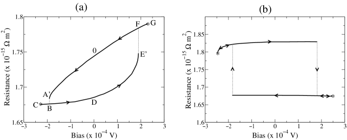
Figure 12: Resistance of the Co/Cu/Co(111) junction as a function of the applied current, with $M=1$ monolayer of Co in the switching magnet. (a) is for $\theta=2$rad and (b) for $\theta=3$rad.

However the ratio $r\approx-1$ is now negative and the hysteresis loops in Fig. 12 illustrate the interesting behaviour discussed in Section III when the system subjected to a bias higher than a critical bias moves to the ”both unstable” region shown in Fig. 6. As in Fig. 7 the points on the hysteresis loop in Fig. 12 corresponding to the critical bias are labelled by asterisks. Fig. 12(b) and Fig. 7(a) are in close correspondence because Fig. 7(a) is for $r_{\rm c}<r<0$ and in the present case $r=-1$, $r_{\rm c}=-2/(\gamma h_{\rm p})=-2$. Also, from Fig. 9(a), $g_{\parallel}<0$ so that $vg_{\parallel}$ in Fig. 7(a) has the same sign as the voltage $V$ in Fig. 12(b).

VI Summary

Spin-transfer torque is responsible for current-driven switching of magnetisation in magnetic layered structures. The simplest theoretical scheme for calculating spin-transfer torque is a generalised Landauer method and this is used in Section II to obtain analytical results for a simple model. The general phenomenological form of spin-transfer torque is deduced in Section III and this is introduced into the Landau-Lifshitz-Gilbert equation, together with torques due to anisotropy fields. This describes the motion of the magnetisation of the switching magnet and the stability of the steady states (constant current and stationary magnetisation direction) is studied under different experimental conditions, with and without external field. This leads to hysteretic and reversible behaviour in resistance versus bias (or current) plots in agreement with a wide range of experimental observations. In Section IV the general principles of a self-consistent treatment of spin-transfer torque are discussed and the Keldysh formalism for quantitative calculations is introduced. This approach to the non-equilibrium problem of electron transport uses Green functions which are very convenient to calculate for a realistic multiorbital tight-binding model of the layered-structure. In Section V quantitative calculations for Co/Cu/Co(111) systems are presented which yield switching currents of the observed magnitude.

This study of current-driven switching of magnetisation was carried out in collaboration with J. Mathon and A. Umerski and financial support was provided by the UK Engineering and Physical Research Council (EPSRC).

References

- (1) P. Grünberg, R. Schreiber, Y. Pang, M. B. Brodsky, and H. Sower, Phys. Rev. Lett. 57, 2442 (1986); M. N. Baibich, J. M. Broto, A. Fert, Van Dau Nguyen, F. Petroff, P. Etienne, G. Creuset, A. Friederich, and J. Chazelas, Phys. Rev. Lett. 61, 2472 (1998)
- (2) S. S. P. Parkin et al., J. Appl. Phys. 85, 5828 (1999).
- (3) J. C. Slonczewski, J. Magn. Magn. Mater. 159, L1 (1996).
- (4) X. Waintal, E. B. Myers, P. W. Brouwer, and D. C. Ralph, Phys. Rev. B 62, 12317 (2000)
- (5) e.g. “Transport in Nanostructures” by D. K. Ferry and S. M. Goodnick (Cambridge University Press 1997).
- (6) J. Z. Sun, Phys. Rev. B 62, 570 (2000).
- (7) F. J. Albert, J. A. Katine, R. A. Buhrman, and D. C. Ralph, Appl. Phys. Lett. 77, 3809 (2000).
- (8) J. Grollier, V. Cross, A. Hamzic, J. M. George, H. Jaffres, A. Fert, G. Faini, J. Ben Youssef, and H. Le Gall, Appl. Phys. Lett. 78, 3663 (2001).
- (9) E. C. Stoner and E. P. Wohlfarth, Phil, Trans. Roy. Soc. A 240, 599 (1948).
- (10) J. Grollier, V. Cross, H. Jaffres, A. Hamzic, J. M. George, G. Faini, J. Ben Youssef, H. Le Gall, and A. Fert, Phys. Rev. B 67, 174402 (2003).
- (11) F. J. Albert, N. C. Emley, E. B. Myers, D. C. Ralph, and R. A. Buhrman, Phys. Rev. Lett. 89, 226802 (2002).
- (12) D. W. Jordan and P. Smith, Nonlinear Ordinary Differential Equations, Clarendon Press, Oxford (1977).
- (13) D. M. Edwards, F. Federici, G. Mathon, and A. Umerski, Phys. Rev. B 71, 134501 (2005).
- (14) J.A. Katine, F. J. Albert, R. A. Buhrman, E. B. Myers, and D. C. Ralph, Phys. Rev. Lett. 84, 3149 (2000).
- (15) S. I. Kiselev, J. C. Sankey, I. N. Krivorotov, N. C. Emley, R. J. Schoelkopf, R. A. Buhrman, and D. C. Ralph, Nature 425, 380 (2003).
- (16) S. Urazhdin, N. O. Birge, W. P. Pratt, Jr., and J. Bass, Phys. Rev. Lett. 91, 146803 (2003)
- (17) M. R. Pufall, W. H. Rippard, S. Kaka, S. E. Russek, T. J. Silva, J. Katine, and M. Carey, Phy. Rev. Lett. 69, 214409 (2004).
- (18) E. B. Myers, F. J. Albert, J. C. Sankey, E. Bonet, R. A. Buhrman, and D. C. Ralph, Phys. Rev. Lett. 89, 196801 (2002)
- (19) M. A. Zimmler, B. Özyilmaz, W. Chen, A. D. Kent, J. Z. Sun, M. J. Rooks, and R. H. Koch, Phy. Rev. B 70, 184438 (2004).
- (20) M. Tsoi, A. G. M. Jansen, J. Bass, W. C. Chiang. M. Seck, V.Tsoi, and P. Wyder, Phys. Rev. Lett. 80, 4281 (1998).
- (21) M. Tsoi, A. G. M. Jansen, J. Bass, W. C. Chiang. V. Tsoi, and P. Wyder, Nature 406, 46 (2000)
- (22) E. B. Myers, D. C. Ralph, J. A. Katine, R. N. Louie and R. A. Buhrman, Science 285, 867 (1999).
- (23) J. C. Slonczewski, J. Magn. Magn. Mater. 195, L261 (1999); 247, 324 (2002).
- (24) B. Özyilmaz, A. D. Kent, D. Monsma, J. Z. Sun, M. J. Rooks, and R. H. Koch, Phys. Rev. Lett. 91, 067203 (2003).
- (25) M. Tsoi, J. Z. Sun, M. J. Rooks, R. H. Koch, and S. S. P. Parkin, Phys. Rev. B 69, 100406(R) (2004).
- (26) W. F. Brown, Phys. Rev. B 130, 1677 (1963).
- (27) Z. Li and S. Zhang, Phys. Rev. B 69, 134416 (2004).
- (28) J. Miltat, G. Albuquerque, A. Thiaville, and C. Vouille, J. Appl. Phys. 89, 6982 (2001).
- (29) Z. Li and S. Zhang, Phys. Rev. B 68, 024404 (2003).
- (30) C. R. P. Cowburn, C. K. Koltsov, A. O. Adeyeye, and M. E. Welland, Phys. Rev. Lett. 83, 1042 (1999).
- (31) Y. Jiang, S. Abe, T. Ochiai, T. Nozaki, A. Hirohata, N. Tezuka, and K. Inomata, Phys. Rev. Lett. 92, 167204 (2004).
- (32) Y. Jiang, T. Nozaki, S. Abe, T. Ochiai, A. Hirohata, N. Tezuka, and K. Inomata, Nature Materials 3, 361 (2004).
- (33) N. Tezuka (private communication)
- (34) K. Capelle and B. L. Gyorffy, Europhys. Lett. 61, 354 (2003).
- (35) J. Sun, Nature 424, 359 (2003).
- (36) J. Mathon, Murielle Villeret, A. Umerski, R. B. Muniz, J. d’Albuquerque e Castro, and D. M. Edwards, Phys. Rev B, 56, 11797 (1997).
- (37) J. Mathon, Murielle Villeret, R. B. Muniz, J. d’Albuquerque e Castro, and D. M. Edwards, Phys. Rev. Lett. 74, 3696 (1995).
- (38) S. Zhang, P. M. Levy, and A. Fert , Phys. Rev. Lett. 88,236601 (2002).
- (39) A. A. Kovalev, A. Brataas, and G. E. W. Bauer, Phys. Rev. B 66 , 224424 (2002).
- (40) D. M. Edwards and J. Mathon in ”Nanomagnetism: Multilayers, Ultrathin Films and Textured Media”, eds. J. A. C. Bland and D. L. Mills (Elsevier, to be published).
- (41) L. V. Keldysh, Sov. Phys. JETP, 20, 1018 (1965).
- (42) C. Caroli, R. Combescot, P. Nozieres, and D. Saint-James, J. Phys. C 4, 916 (1971).
- (43) D. M. Edwards in: Exotic states in quantum nanostructures, ed. by S. Sarkar, Kluwer Academic Press (2002).
- (44) G. D. Mahan, Many Particle Physics, 2nd Ed., Plenum Press, New York (1990).