Consensus Formation in Multi-state Majority and Plurality Models

Abstract

We study consensus formation in interacting systems that evolve by multi-state majority rule and by plurality rule. In an update event, a group of $G$ agents (with $G$ odd), each endowed with an $s$-state spin variable, is specified. For majority rule, all group members adopt the local majority state; for plurality rule the group adopts the local plurality state. This update is repeated until a final consensus state is generally reached. In the mean field limit, the consensus time for an $N$-spin system increases as $\ln N$ for both majority and plurality rule, with an amplitude that depends on $s$ and $G$. For finite spatial dimensions, domains undergo diffusive coarsening in majority rule when $s$ or $G$ is small. For larger $s$ and $G$, opinions spread ballistically from the few groups with an initial local majority. For plurality rule, there is always diffusive domain coarsening toward consensus.

I Introduction

A simple description for consensus in an interacting population is based on endowing each individual, or agent, with discrete opinion states that evolve by kinetics in which neighboring agents tend to agree. Perhaps the best studied such example is the 2-state voter model voter , in which a randomly-selected agent adopts the state of one of its neighbors. This update is repeated until a finite system necessarily reaches consensus. When the densities of agents of each state are equal, the time to reach consensus in $d$ dimensions scales linearly in the number of agents $N$ for $d>2$, as $N\ln N$ for $d=2$, and as $N^{2/d}$ for $d<2$ voter ; pk . Another classical description for consensus formation is the Ising model with zero-temperature Glauber kinetics glauber . Here, a randomly-picked agent adopts the state of the majority in its local interaction neighborhood; in case of a tie, the initial agent flips with probability 1/2. While this updating promotes agreement, consensus does not necessarily arise. In fact, the system almost always gets stuck in infinitely long-lived metastable states for spatial dimension $d\geq 3$ SKR .

Recently, another prototypical model for consensus formation, majority rule (MR), was introduced galam . In MR, a system consists of 2-state agents, corresponding to two distinct opinions. Agents evolve by the following two steps: first, pick a group of agents with fixed odd size $G$; this group is an arbitrary set of agents in the mean-field limit, or a contiguous group for finite spatial dimension. Second, all agents in this group adopt the local majority state. These two steps are repeated until consensus is reached MM ; MR2D . The MR model is analogous to the majority rule of the Ising model with zero-temperature Glauber kinetics, except that more than one agent can flip in a single update step. A related multi-spin kinetics occurs in the Sznajd model szn , where a small contiguous group of same-species spins induces all spins on the group boundary to flip. A perhaps desirable feature of the MR model is that the group-based kinetics ensures that consensus is always reached in a finite system.

Figure 1: Illustration of a single update in majority and in plurality rule for a $3$-state system with group size $G=7$.

In this work, we study two natural extensions of majority rule (Fig. 1). The first is to allow each agent to have more than 2 equivalent states, i.e., each agent possesses a Potts-like opinion variable that may be in any of $s$ states $a,b,c,\ldots,s$ GGP . The update step is similar to that in the original MR model. A group of $G$ agents, with $G$ an odd number, is first identified. If a local majority in this group exists, that is, if $(G+1)/2$ or more agents in the group are in a single state, then all agents adopt this local majority state. However, if there is no local majority, then the group does not evolve. A new feature of the multi-state compared to the 2-state model is the possibility of static groups in which there is no local consensus. Because of this feature, a finite system does not necessarily reach consensus. One of our goals will be to characterize the dynamics of MR with more than 2 states and to determine whether the final outcome is consensus or a frozen state.

A second extension is plurality rule (PR), which is meaningful only if the number of spin states is 3 or greater. In a single update step of PR, a group of size $G$ is first identified. Next the state with the most representatives in that group—the plurality state—is determined. All agents in this group then adopt this plurality state. In case of a tie, the agents all adopt one of the multiple plurality states equiprobably. This type of evolution mimics how consensus might be achieved in parliamentary systems when there are more than two parties. Clearly, the PR model avoids the freezing phenomenon that can occur in the multistate MR model. We will investigate how the PR model approaches consensus and the basic differences between MR and PR dynamics.

In Sec. II, we study the MR and PR models in the mean-field limit and show generically that the consensus time grows logarithmically with $N$. Then in Sec. III, we discuss the change from diffusive domain coarsening, when the number of opinion states $s$ and the group size $G$ are small, to ballistic domain evolution, and finally to no evolution as $s$ and $G$ increase. In Sec. IV, we present simulation results about the consensus time distribution for the multi-state MR model that illustrate these two regimes of behavior. In Sec. V, we discuss the dynamical behavior of the PR and compare with the MR model. We conclude in Sec. VI.

II Mean-field limit

II.1 Two-State Model

We begin with the mean-field solution for the 2-state MR model in the continuum $N\to\infty$ limit. While the mean-field solution for the $2$-state MR model with a finite number of agents was obtained previously MM , the continuum solution is much simpler, while still exhibiting nearly all of the features of the discrete solution.

For simplicity, consider first the case of group size $G=3$. In an update step, the number of agents in state $a$, $N_{a}$, increases by 1 if the group state is $aab$, while this number of agents decreases by 1 if the group state is $bba$. Thus $dN_{a}\!=3(a^{2}b-ab^{2})$, where $a$ and $b$ now denote the global densities of agents of each type, and the factor of 3 accounts for the 3 permutations of agents in the group. If there is local consensus in a group, then $N_{a}$ does not change in an update. We increment the time by $dt=3/N$ in an update so that each agent typically flips once in a single time unit. With these preliminaries, the rate equations for the agent densities are

$$\dot{a} = a^{2}b-b^{2}a$$

$$\dot{b} = b^{2}a-a^{2}b.$$ (1)

Since the total density $a+b=1$, we rewrite Eq. (II.1) as

$$\dot{a}=ab(a-b)=-2a\left(a-1/2\right)(a-1).$$ (2)

In the latter form, we see that $a=0,1$ are stable fixed points, while $a=1/2$ is unstable. Thus starting from any $a\neq 1/2$, the system is quickly driven to consensus because of the non-zero bias inherent in Eq. (2). The existence of a bias contrasts with the voter model, where the average magnetization is conserved voter , and purely diffusive dynamics governs the evolution.

To determine the time until consensus is reached, we rewrite Eq. (2) in the partial fraction expansion

$$\left[\frac{1}{a}+\frac{1}{a-1}-\frac{2}{a-\frac{1}{2}}\right]\,da=-dt$$ (3)

and integrate this equation of motion between suitable initial and final states. To describe a finite system of $N$ agents, we chose $a_{0}=\frac{1}{2}+\frac{1}{N}$ and $a_{\infty}=1-\frac{1}{N}$, corresponding to the initial densities of the two species being equal and a final state of consensus. Integrating Eq. (3) over this range, we obtain

$$t\sim 3\ln N.$$ (4)

Thus, as previously found in the exact discrete solution MM , the consensus time $t$ scales as $\ln N$. This dependence is a consequence of the driving force in Eq. (2) vanishing linearly as a function of the distance to the fixed points $a=0,1/2$, and $1$. However, the dependence of the amplitude in the consensus time is different in the discrete and continuum solutions. In the former case, the amplitude suddenly drops from 2 to 1 as $|a-1/2|$ becomes larger than ${\cal O}(1/\sqrt{N})$ MM , while in the continuum solution, the amplitude changes from 3 to 1 as $a-1/2$ becomes comparable to either $a$ or $1-a$.

The above considerations can be extended to larger group sizes. By laborious enumeration of all states up to $G=11$, it appears that the extension of Eq. (2) to general group size is

$$\dot{a}=ab(a-b)\left[1+3ab+10(ab)^{2}+\ldots+\left(\!\!{j\atop{\frac{j+1}{2}}}\!\!\right)(ab)^{(j-1)/2}\right],$$ (5)

where $j=G-2$. Using Stirling’s approximation, the higher-order terms are all ${\cal O}(1/\sqrt{G})$ and there are ${\cal O}(G)$ such terms. Thus near the unstable fixed point, namely $a=\frac{1}{2}(1+\epsilon)$, the equation of motion reduces to

$$\dot{\epsilon}\propto\frac{\epsilon}{2}\sqrt{G}.$$ (6)

Thus for general group size $G\ll N$, the time to reach consensus should scale as $(\ln N)/\sqrt{G}$.

II.2 More Than Two States

We now extend our considerations to the multi-state MR model. Consider first the simplest case of 3 states ($s=3$) and group size $G=3$. In the same spirit as Eq. (2), the rate equations for this 3-state model are

$$\dot{a} = a^{2}(b+c)-a(b^{2}+c^{2})$$

$$\dot{b} = b^{2}(c+a)-b(c^{2}+a^{2})$$

$$\dot{c} = c^{2}(a+b)-c(a^{2}+b^{2}),$$ (7)

with the densities of these states subject to the normalization condition $a+b+c=1$.

To understand the resulting dynamics, we examine the stability of the fixed points in these rate equations. There are 7 such points; a globally unstable fixed point at $U\equiv(\frac{1}{3},\frac{1}{3},\frac{1}{3})$, three saddle points $S_{ab}\equiv(\frac{1}{2},\frac{1}{2},0)$, $S_{ac}\equiv(\frac{1}{2},0,\frac{1}{2})$, and $S_{bc}\equiv(0,\frac{1}{2},\frac{1}{2})$, and 3 stable points $A\equiv(1,0,0)$, $B\equiv(0,1,0)$, and $C\equiv(0,0,1)$ (Fig. 2). There are 3 separatrices that join the unstable fixed point to each of the saddle points (Fig. 2).

Figure 2: The phase plane $a+b+c=1$ in density space, showing the unstable fixed point ($\circ$), saddle points ($\square$), and stable fixed points ($\bullet$). Separatrices are shown dashed. Typical flows near the separatrices are also shown.

We now compute the time to reach consensus starting from the unstable fixed point. There are two natural choices for the path to consensus. One is to run from the unstable fixed point to a saddle point close to a separatrix, and then flow to the stable fixed point, as shown in Fig. 2. This path, $(\frac{1}{3},\frac{1}{3},\frac{1}{3})\to(\frac{1}{2},\frac{1}{2},0)\to(1,0,0)$, corresponds to one species disappearing first, while the other two have the same density, before ultimate consensus is reached. The other is the direct route $(\frac{1}{3},\frac{1}{3},\frac{1}{3})\to(1,0,0)$ along a path where $b=c$. That is, $b$ and $c$ both disappear at the same rate as consensus is reached.

For the indirect route, we first calculate the time required to go from $U$ to $S_{ab}$. With the conditions $a=b$ and $c=1-2a$, the first of Eqs. (II.2) can be rewritten as

$$\dot{a} = a^{2}[a+(1-2a)]-a[a^{2}+(1-2a)^{2}]$$ (8)

$$= -6a(a-1/2)(a-1/3).$$

Thus the time until the $c$ density vanishes is

$$t_{c} \approx \int^{\frac{1}{2}-\frac{1}{N}}_{\frac{1}{3}+\frac{1}{N}}\left[-\frac{1}{a}-\frac{2}{a-\frac{1}{2}}+\frac{3}{a-\frac{1}{3}}\right]\,da$$ (9)

$$= -2\ln(6/N)+3\ln(N/6)-6\ln(3/2)$$

$$\approx 5\ln N.$$

Once again, the integration limits are chosen to correspond to the system being infinitesimally close to, but not exactly at the fixed points at either end of the trajectory. Similarly, the time to go from $S_{ab}$ to $A$ asymptotically scales as $3\ln N$. Thus the total time to go from $(\frac{1}{3},\frac{1}{3},\frac{1}{3})$ to consensus asymptotically scales as $8\ln N$. Following the same line of reasoning, the consensus time from $(\frac{1}{3},\frac{1}{3},\frac{1}{3})$ to $(1,0,0)$ directly along the path where $b=c$ always, asymptotically scales as $4\ln N$.

For the case $G=3$, we may generalize to obtain the consensus time for an arbitrary number of states $s$. The rate equations (II.2) become

$$\dot{a}_{1}=a_{1}^{2}(a_{2}+a_{3}+\cdots+a_{s})-a_{1}(a_{2}^{2}+a_{3}^{2}+\cdots+a_{s}^{2}),$$ (10)

plus cyclic permutations. Here $a_{k}$ now denotes the density of the $k^{\rm th}$ species. Again, we compute the consensus time along a sequential path in which one species disappears first while the remaining species have equal densities, as well as along a direct path in which $s-1$ species have equal densities that all go to zero simultaneously.

For the first leg of the sequential path, the densities satisfy the conditions $a_{1}=a_{2}=a_{3}=\cdots=a_{s-1}=a$ and $a_{s}=1-(s-1)a$. Then Eq. (10) reduces to

$$\dot{a}=-s(s-1)\,\,a\left(a-\frac{1}{s-1}\right)\left(a-\frac{1}{s}\right).$$ (11)

Integrating from the unstable fixed point to the fixed point where the density of one species is zero, the transit time equals $(2s-1)\ln N$. Repeating this calculation as each species is eliminated, the consensus time is

$$t=\sum_{k=2}^{s}(2k-1)\ln N=(s^{2}-1)\ln N$$ (12)

Similarly, for consensus via a direct path, the densities satisfy the constraints $a_{1}=a$ and $a_{2}=a_{3}=\cdots=a_{s}=(1-a)/(s-1)$. Now Eq. (10) becomes

$$\dot{a}=-\frac{s}{s-1}\,\,a\left(a-\frac{1}{s}\right)\left(a-1\right),$$ (13)

from which the consensus time equals $(s+1)\ln N$.

In summary, the consensus time always scales as $\ln N$, with a prefactor that is an increasing function of the number of states. This coefficient depends on the actual route to consensus. If species are eliminated one by one, the coefficient grows quadratically with $s$, while if one species dominates and the remaining $s-1$ all disappear at the same rate, the coefficient grows linearly with $s$. Qualitatively similar results arise for larger group sizes.

II.3 Plurality Rule

Finally, we study plurality rule (PR) which first becomes distinct from MR when number of states $s\geq 3$ and the group size $G\geq 5$. Let us study this case $s=3,G=5$ for simplicity. By enumerating all group states, the rate equations for the PR model are:

$$\begin{split}\dot{a}&\!=\!a^{4}(b\!+\!c)\!+\!4a^{3}(b\!+\!c)^{2}\!-\!4a^{2}(b^{3}\!+\!c^{3})\!-\!4abc(b^{2}\!+\!c^{2})\\ &~{}~{}~{}~{}-a(b^{4}+c^{4})+3a^{2}bc(b+c)-6ab^{2}c^{2},\\ \end{split}$$ (14)

plus cyclic permutations for $\dot{b}$ and $\dot{c}$. The rate equations for the MR model for $s=3$ and $G=5$ are identical to Eq. (14) except that the last two terms, corresponding to states with no global majority, are absent.

The MR and PR models both share the same global fixed point structure and stability. Let us now determine the transit time from $(\frac{1}{3},\frac{1}{3},\frac{1}{3})\to(\frac{1}{2},\frac{1}{2},0)$ along the path $a=b$ for the case $s=3,G=5$ for both the PR and MR models. Using $a=b$ and $c=1-2a$, the rate equation for $\dot{a}$ reduces to

$$\dot{a} = 48a^{5}-66a^{4}+25a^{3}-a\quad({\rm MR})$$

$$\dot{a} = 36a^{5}-60a^{4}+25a^{3}-a\quad({\rm PR})$$ (15)

To determine the transit time simply, note that the driving flow in the rate equation vanishes linearly near the fixed points and that the coefficient of the linear dependence determines the coefficient of $\ln N$ in the transit time. We thereby find $t\sim 5\ln N$ for PR, while $t\sim\frac{43}{5}\ln N$ for MR. As expected, PR evolves faster than MR because there are fewer possibilities for frozen groups. Finally, to reach consensus via $(\frac{1}{2},\frac{1}{2},0)\to(1,0,0)$, the rate equations for both the PR and MR models are $\dot{a}=6a^{5}-15a^{4}+10a^{3}-a$, so that the time to go from $S_{ab}$ to $A$ is $\frac{23}{7}\ln N$. Thus the consensus time from $U$ is $\frac{58}{7}\ln N$ for PR and $\frac{86}{7}\ln N$ for MR. Thus there is only a quantitative difference between the PR and MR models in the mean-field limit.

III Diffusive vs. Deterministic Consensus

We now investigate the multi-state MR model on the square lattice. While the rate equations predict that the number of states and the group size do not qualitatively affect the evolution, simulations on the square lattice show very different behaviors for systems with small $s$ and/or $G$ and those with large $s$ and $G$ (Figs. 3 & 4). In the former case, a coarsening domain mosaic evolves diffusively. However, when both $s$ and $G$ are large, it is improbable that a small system will contain even a single group with an initial local majority, and such a system will be static. At the boundary between these two regimes, there will typically be a single initial local majority group. When this occurs, there is nearly deterministic evolution in which this group grows ballistically and overruns the system (Fig. 4).

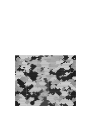
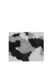
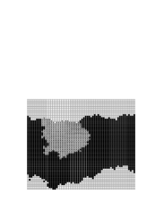
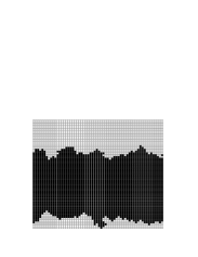
Figure 3: Evolution of a $60\times 60$ 3-state MR model with group size $G=3$ at times $t=1,20,80$, and 640.

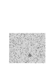
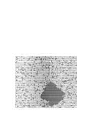
Figure 4: Evolution of a $60\times 60$ 9-state MR model with group size $G=25$ at times $t=0.1,1.5,1.8$, and 2

To delineate these two regimes, we determine the criterion for the existence of at least one group with a local majority in the initial state. As a preliminary, we determine the probability ${\cal P}_{>}$ that a local majority exists in a single group of size $G$, i.e., $n>G/2$ of the agents in the group all have the same opinion. The probability for this event to occur is

$${\cal P}_{>}=s\sum_{n>G/2}^{G}\frac{G!}{n!(G-n)!}\left(\frac{1}{s}\right)^{n}\left(1-\frac{1}{s}\right)^{G-n}.$$ (16)

Using Stirling’s approximation, this expression reduces to

$${\cal P}_{>}\approx 2^{G}\,\frac{(s-1)^{G/2}}{s^{G-1}}\,\sqrt{\frac{2}{\pi G}}\int_{0}^{\infty}e^{-2x^{2}/G}\,e^{-x\ln(s-1)}\,dx,$$ (17)

where $x=n-G/2$ and we extend the upper limit of $x$ from $G/2$ to $\infty$.

For $s=2$, Eq. (17) gives ${\cal P}_{>}=1$, the obvious exact result, suggesting that this Gaussian approximation may be relatively accurate. Conversely, for large $s$, the exponential in the integrand of Eq. (17) decays more rapidly than the Gaussian factor, and we obtain

$${\cal P}_{>}\approx\frac{s}{\sqrt{G}\ln s}\left(\frac{2}{\sqrt{s}}\right)^{G}\qquad s\to\infty.$$ (18)

In fact, for $s=3$, the exponential cutoff controls the integral in Eq. (17) already for $G\approx 4$; for $s=4$, the exponential cutoff dominates for $G\approx 2.23$. Thus the approximate form Eq. (18) is relatively accurate, except the special case $s=2$. Clearly, the probability that a randomly-populated group of size $G$ has a majority decreases rapidly when either $s$ or $G$ increases.

The condition on the number of agents $N$ for there to be at least one initial group in the system that contains a local majority is thus $M{\cal P}_{>}>1$ (Fig. 5), where $M$ is the number of independent groups in the system. While we do not know $M$ exactly, trivial bounds are $N/G\leq M\leq N$. The lower bound is based counting the $N/G$ contiguous groups that tile the system as independent, while the latter is based on considering all $N$ embeddings of the group on the lattice as independent. Since ${\cal P}_{>}$ varies rapidly with $s$ and $G$, this small indeterminacy in $M$ does not play a major role in the condition for the existence of a group with a local majority.

Figure 5: Phase diagram for the majority rule model as a function of the number of states $s$ and the group size $G$. The curves are defined by the criterion $NP_{>}=1$, separates a region of diffusive dynamics (multiple initial majority groups) from a static region (no initial majority groups). The dots correspond to the two parameter values simulated in Sec. IV.

From Eq. (18), the criterion $M{\cal P}_{>}>1$ becomes

$$M>M_{c}\approx\frac{\sqrt{G}\ln s}{s}\,e^{G\ln(\sqrt{s}/2)}.$$ (19)

For $M>M_{c}$, the number of initial groups with a local majority is non-zero so that evolution occurs. If $M<M_{c}$, no groups have a local majority and the system will therefore be static. When $M\gtrsim M_{c}$, majority groups are widely separated and there is a two-stage approach to consensus. First, initial majority groups grow ballistically until they meet, after which domain interfaces evolve diffusively toward final consensus. The case $M\approx M_{c}$ is exceptional as there is typically a single initial group with a local majority that quickly overruns the system (Fig. 4). It is also noteworthy that for moderate values of $s$ and $G$, an astronomically large system is needed for there to be at least one group with a local majority.

Figure 6: Probability for a successful realization versus system size for $s=9,G=25$ MR model based on using $M={N}/{8}$. The error bars are based on a $5\%$ significance level.

To test Eq. (19), we compare our analytical prediction for the “success” probability $P_{\rm success}=1-(1-P_{>})^{M}$, defined as the probability that a randomly-prepared configuration contains at least one majority group, with corresponding simulation data from the $s=9,G=25$ MR model (Fig. 6). We observe that $P_{\rm success}$ increases quickly when the system size passes through the threshold value $M_{c}$, and that there is excellent agreement between the data and our analytics.

IV Consensus Time Distribution in Two Dimensions

We now study the evolution of the multi-state MR model on the square lattice by numerical simulations. We construct a group by incorporating successive diamond-shaped shells with increasing values of $|x|+|y|$, where $x$ and $y$ are the horizontal and vertical distances from the central agent. Thus for a given $G$, the group is defined as the initial agent, plus the 4 agents in the first shell, the 8 agents in the second shell, etc., until a total of $G$ agents are included. To ensure that a group contains precisely $G$ agents, a randomly-selected set of agents in the last shell are typically included. We then evolve the system according to majority rule until consensus is reached.

Figure 7: Probability distribution for the consensus time $P_{N}(t)$ versus $t$ on a square lattice of $N=3600$ sites by majority rule for the two cases of $s=3,G=3$ with data integrated over bins of width $200$ (top), and $s=9,G=25$, and bin size $0.05$ (bottom). The inset shows detail near the peak where the width of the data bins is 2.

As in our previous study of the 2-state MR MR2D , we focus on the distribution of consensus times, $P_{N}(t)$. To illustrate the behavior in the two regimes of Fig. 5, we consider the representative cases $s=3,G=3$ and $s=9,G=25$, with $N=3600$ agents for both examples (heavy dots in Fig. 5), in which the initial concentrations of all species are equal. As shown in Fig. 7, there is a long-time tail in $P_{N}(t)$ for the $3$-state model that is qualitatively similar to that in the $2$-state model. For 3 states, approximately 1/5 of all configurations get stuck in long-lived coherent stripe states, compared to approximately 1/3 of all states in the $2$-state model MR2D . Analogous coherent states, albeit with infinite lifetimes, also occur in the Ising model with zero-temperature Glauber kinetics SKR .

Figure 8: Dependence of the two characteristic times $T_{\rm mp}$ ($\Box$) and $\tau$ ($\circ$) on $N$ for the 3-state $G=3$ MR model.

For the 3-state model, we also measure the $N$-dependence of the two basic time scales: (a) the most probable consensus time, $T_{\rm mp}\equiv e^{\langle\ln t\rangle}$, corresponding to the location of the peak in $P_{N}(t)$, and (b) the characteristic decay time in the exponential tail of $P_{N}(t)\sim e^{-t/\tau}$. As found previously for the 2-state model MM ; MR2D , these time scales have power-law dependences on $N$ with different exponents (Fig. 8). By fitting the data to straight lines, we find that $T_{\rm mp}$ varies as $N^{\alpha}$, where $\alpha=1.18\pm 0.03$, while $\tau$ varies as $N^{\beta}$, with $\beta=1.77\pm 0.05$. All quote error bars correspond to a $5\%$ significance level. These exponents are close to the corresponding values of $1.24$, and $1.7$ respectively, quoted for the 2-state model MR2D . We conclude that the same underlying domain wall diffusion mechanism governs the approach to consensus in both the 2- and 3-state MR models.

Figure 9: Dependence of the mean consensus time $\langle t_{N}\rangle$ versus $N$ for $9$-state $G=25$ MR model.

In contrast, for the $s=9,G=25$ MR model, the consensus time distribution is sharply peaked about its most probable value (Fig. 7), so that there is only a single characteristic time scale. The absence of a second longer time scale is due to the fact that long-lived configurations, such as stripe states, no longer occur. We find that the average consensus time grows only as $N^{\alpha}$, with $\alpha=0.48\pm 0.04$ (Fig. 9). Since we are interested in the $N$-dependence of the consensus time for large $N$, where almost all configurations are successful, we define this average only for successful realizations.

We can justify the slow growth of the consensus time for the case $s=9,G=25$ by a simple-minded argument. Since the evolution is determined by the growth of a single domain, the consensus time is essentially the time for this domain to overrun the system. According to majority rule, a randomly selected group typically evolves when more than half of its area is within the dominating domain. Thus after each time step, the radius of this domain grows by an amount that is of the order of $G$. When the domain radius equals the linear dimension of the system, $Gt=\sqrt{N}$, and consensus is reached. Thus we obtain $t\approx{\sqrt{N}}/{G}$, which appears to account for the $N$-dependence of the consensus time in Fig. 9.

V Majority vs. Plurality Rule

We now study the plurality rule (PR) model when the spatial dimension is finite. While the MR and PR models behave similarly in the mean-field limit, they evolve quite differently when the spatial dimension is finite, as seen by comparing single realizations of the system that evolve according to PR (Fig. 10) and according to MR (Fig. 4), with $s=9,G=25$ for both examples.

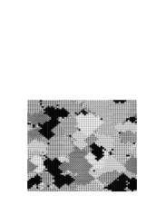
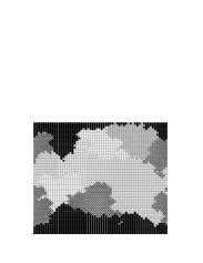
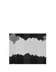
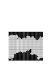
Figure 10: Evolution of a $60\times 60$ 9-state PR model with group size $G=25$ at times $t=0.1,1,4$, and 20

By construction, all configurations in the PR model are active, since a plurality exists in any group, independent of the number of states and the group size. Thus the PR model always evolves by diffusive domain coarsening. When only two states remain, the ensuing evolution is exactly that of the 2-state MR model. As in the case of the 2-state MR model, we therefore expect that a non-negligible fraction of all realizations will get stuck in a stripe-like state, an example of which is given in Fig. 10.

Figure 11: Probability distribution for the consensus time $P_{N}(t)$ versus $t$ on a square lattice of $N=3600$ sites by plurality rule for the two cases of $s=3,G=3$, with data integrated over bins of width $100$ (top), and $s=9,G=25$, and bin size $0.2$ (bottom). The inset shows detail near the peak where the width of the data bins is 2.

As a result of the correspondence with majority rule in the long-time limit, the distribution of consensus times should again be characterized by two time scales – the most probable consensus time and the time associate with the asymptotic decay of the consensus time distribution itself. For the case of $s=3,G=3$, the consensus time distributions in the MR and PR models are quantitatively similar (compare the top panels of Figs. 7 and 11) and the behaviors of the two basic time scales in the distribution are also nearly the same. The actual values of $T_{\rm mp}$ and $\tau$ in these two models are quite close, with ${T_{\rm mp}^{\rm PR}}/{T_{\rm mp}^{\rm MR}}=0.92$ and ${\tau^{\rm PR}}/{\tau^{\rm MR}}=0.98$. As expected, the times are smaller in the PR model because every groups is necessarily active, in contrast to the situation in majority rule.

As the number of states is increased, the consensus time distribution in PR continues to be described by two distinct time scales. An example for the case of the $s=9,G=25$ PR model is shown in Fig. 11, whose behavior strongly contrasts that of the $s=9,G=25$ MR model (bottom panel in Fig. 7). A final feature worth noting is that the characteristic time scales decrease with $G$, reflecting the fact that larger groups necessarily lead to quicker consensus formation.

VI Summary and Discussion

We studied two extensions of the 2-state majority rule (MR) model for consensus formation, namely, multi-state majority rule (MR) and plurality rule. In the mean-field limit, both these models reach consensus in a time that grows logarithmically with the number of agents $N$. Variations in the microscopic evolution rules, such as majority or plurality rule, the number of spin states $s$, and the group size $G$, merely lead to a quantitative difference in the amplitude of $\ln N$ in the consensus time.

For finite spatial dimension, the MR model has two distinct regimes of behavior that are delineated by the relative values of $s$, $G$, and $N$. For small $s$ or small $G$, many groups have local majorities in a typical initial state. These groups are the nuclei of domains whose long-time dynamics is governed by diffusive coarsening. For this range of $s$ and $G$, the multi-state MR model thus evolves in a manner similar to that in the $2$-state MR model. The distribution of consensus times has two widely separated time scales – the most probable consensus time and the asymptotic decay time of the consensus time distribution. The dependences of these two time scales on $N$ is quite close to those in the 2-state MR model.

On the other hand, for sufficiently large $s$ and $G$, it becomes prohibitively unlikely that a finite system will contain even a initial single group with a local majority. Thus essentially all realizations of the system are frozen. As the boundary between these two regimes is approached, a typical realization will contain either zero or one initial group with a local majority. In the latter case, this domain quickly imposes its state on the entire system. This phenomenon has a number of unfortunate historical examples, such as Germany in 1933, Italy in 1922, and Russia in 1917, where a well-organized, extremist, and initially minority party ultimately imposed its will upon a deadlocked political system.

We also investigated the dynamics of plurality rule (PR), where a group adopts the state of its plurality members in an update event. In the mean-field limit, PR and MR were observed to have qualitatively similar behavior. For finite spatial dimension, however, all groups in PR are active. Thus the evolution of the system for any $s$ and $G$ is qualitatively similar to that of MR in which the number of states and the group size is small. As one should expect, a voting system based on plurality rule facilitates the achievement of ultimate consensus.

- (1) T. M. Liggett, Interacting Particle Systems (Springer-Verlag, New York, 1985).
- (2) P. L. Krapivsky, Phys. Rev. A 45, 1067 (1992).
- (3) R. J. Glauber, J. Math. Phys. 4, 294 (1963).
- (4) V. Spirin, P. L. Krapivsky, and S. Redner, Phys. Rev. E 63, 036118 (2001); Phys. Rev. E 65, 016119 (2002).
- (5) S. Galam, Physica (Amsterdam) 274, 132 (1999); Eur. Phys. J. B 24, 403 (2002); cond-mat/0211571.
- (6) P. L. Krapivsky and S. Redner, Phys. Rev. Lett. 90, 238701 (2003).
- (7) P. Chen and S. Redner, Phys. Rev. E. 71, 036101 (2005).
- (8) K. Sznajd-Weron and J. Sznajd, Int. J. Mod. Phys. C 11, 1157 (2000); D. Stauffer, J. Artif. Soc. Soc. Simul. 5, no. 1 (2002).
- (9) A related 3-state model where tie-breaking plays a major role in the dynamics was recently studied by S. Gekle, S. Galam, and L. Peliti, cond-mat/0504254.