Critical points and non-Fermi liquids in the underscreened pseudogap Kondo model

Abstract

Numerical Renormalization Group simulations have shown that the underscreened spin-1 Kondo impurity model with power-law bath density of states (DOS) $\rho(\omega)\propto|\omega|^{r}$ possesses various intermediate-coupling fixed points, including a stable non-Fermi liquid phase. In this paper we discuss the corresponding universal low-energy theories, obtain thermodynamic quantities and critical exponents by renormalization group analysis together with suitable $\epsilon$-expansions, and compare our results with numerical data. Whereas the particle-hole symmetric critical point can be controlled at weak coupling using a simple generalization of the spin-1/2 model, we show that the stable non-Fermi liquid fixed point must be accessed near strong coupling via a mapping onto an effective ferromagnetic $S_{{\mathrm{eff}}}=1/2$ model with singular bath DOS with exponent $r_{{\mathrm{eff}}}=-r<0$. In addition, we consider the particle-hole asymmetric critical fixed point, for which we propose a universal field theory involving the crossing between doublet and triplet levels.

I Introduction

Quantum impurity models were introduced in the context of dilute magnetic moments in metals and are based on the notion that important aspects of the physics of extended systems can be captured by spatially local processes. Indeed, the reduction of a complicated many-body problem to the study of a single quantum degree of freedom coupled to a simplified environment can be an important step in understanding more complex physical situations. Impurity models form the basis for the investigation of lattice systems containing local moments – these turn out to be extremely rich, displaying various phenomena such as heavy-electron quantum coherence, glassiness, and quantum phase transitions. In addition, simpler yet interesting quantum effects that take place at the level of a single magnetic moment can also be successfully described using (oversimplified) single impurity models hewson . The fermionic Kondo effect, i.e., the screening of an extra magnetic moment by conduction electrons, is certainly the hallmark of this single-impurity approach, but other aspects like local non-Fermi liquid behavior and boundary quantum phase transitions vojta have also been put forward.

In general, single-impurity models can serve as an excellent testing ground for novel techniques and physical paradigms that may be helpful in the more complicated case of extended or dense impurity systems. In this respect, recent work based on the so-called pseudogap (or gapless) Kondo and Anderson models, in which conduction electrons obey a semi-metallic density of states that vanishes as $\rho(\omega)\propto|\omega|^{r}$ ($r>0$), has shown interesting promises. Indeed, this problem features a plethora of non-trivial properties, which can be elegantly captured by controlled fermionic renormalization group (RG) techniques fradkin ; fritz1 . Powerful non-perturbative Numerical Renormalization Group (NRG) simulations fritz1 ; ingersent were able to confirm the success of the analytical approach. In particular, recent work fritz1 ; fritz2 has exposed that all fixed points appearing in these pseudogap models can be accessed perturbatively after identifying the value of the DOS exponent $r$ that corresponds to their associated lower-critical or upper-critical “dimension”.

While the fixed points of the pseudogap spin-1/2 Kondo and single-orbital Anderson models are now understood in this language, here we are interested in certain extensions of these models for which numerical data is also available: the case of a spin-1 impurity has been investigated in the extensive work of Gonzalez-Buxton and Ingersent ingersent , and has shown interesting yet unexplained properties. We note that the physics of spin-1 Kondo models can be realized in multilevel quantum dot systems, and theoretical predictions for transport quantities reflecting the singular Fermi liquid behavior of underscreened Kondo spins in a metallic host singFL have been put forward anna .

In this paper, our objective is twofold: first, we will generalize the theories for the critical fixed points, which are already present in the spin-1/2 pseudogap Kondo model, to the $S=1$ situation, following Refs. fradkin, ; fritz2, . This includes two types of fixed points, one occuring at particule-hole (p-h) symmetry and being controlled at small $r$, and the other present away from p-h symmetry and captured near $r=1$ using a general mapping onto an effective interacting resonant level model. Second, we describe the physics of the additional stable fixed point which emerges at particle-hole symmetry, due to the instability of the strong-coupling symmetric fixed point for $S>1/2$. Analyzing the leading relevant perturbation, we will be able to capture this non-Fermi phase by a mapping onto an effective ferromagnetic spin $S_{{\mathrm{eff}}}=1/2$ model with singular exponent $r_{{\mathrm{eff}}}=-r<0$. Technically, we will perform one-loop perturbative RG calculations together with suitable $\epsilon$-expansions epsfoot to determine thermodynamic quantities; the results compare favorably with the numerical data obtained in Ref. ingersent, . The present work also illustrates the broad applicability of the general field-theoretic tools, developed in Refs. fradkin, ; fritz1, ; fritz2, , in a more complicated setting.

The bulk of the paper is organized as follows: we start by presenting the spin-1 Kondo model with a given pseudogap density of states (Sec. II), and summarize previous results from NRG calculations (Sec. III). In Sec. IV, we focus on the case of particle-hole symmetry. It shows a critical point accessible from weak coupling (which is a generalization to $S>1/2$ of the critical point analyzed by Withoff and Fradkin fradkin ). We also present an analysis and strong-coupling calculations for the stable non-Fermi liquid fixed point found in the numerical simulations of Ref. ingersent, . Sec. V presents a novel field theory that describes the quantum phase transition between the free-moment and strong-coupling phases in the presence of particle-hole asymmetry. In all cases, direct comparison to NRG data is made. Technical details on the diagrammatic approach can be found in several appendices. We will finally conclude the paper and discuss some open questions related to the pseudogap Kondo model.

II The model

The pseudogap Kondo model (for a review, see Ref. vojta, ) originates from the question of how a magnetic moment reacts to the coupling to an electronic bath which has depleted weight at the Fermi level, and is of interest to various condensed-matter systems such as $d$-wave superconductors, graphite, and semiconductors. The basic physical idea is that the possibility of observing a Kondo effect is weakened by the lack of low-energy states, which results in various quantum phase transitions controlled by the strength of the Kondo interaction, the amount of particle-hole symmetry breaking, and obviously the shape of the electronic density of states. We will model the latter by the simplified form

$$\rho(\epsilon)=\sum_{k}\delta(\epsilon-\epsilon_{k})=N_{0}|\epsilon|^{r}\theta(D^{2}-\epsilon^{2})\,,$$ (1)

which has an algebraic dependence in energy characterized by the number $r>0$ (the standard Kondo model corresponds to $r=0$). Here $D$ is the half-bandwidth and $N_{0}=(r+1)/(2D^{r+1})$.

The Kondo model is characterized by an antiferromagnetic coupling $J_{B}$ to this fermionic bath, and possibly a potential scattering term $E_{0}$. It reads

$${\cal H}_{B} = \sum_{k\sigma}\epsilon_{k}c^{\dagger}_{k\sigma}c^{\phantom{\dagger}}_{k\sigma}+J_{B}\vec{S}_{B}\cdot\sum_{\sigma\sigma^{\prime}}c^{\dagger}_{\sigma}({\bf 0})\frac{\vec{\tau}_{\sigma\sigma^{\prime}}}{2}c^{\phantom{\dagger}}_{\sigma^{\prime}}({\bf 0})$$ (2)

$$+E_{0}\sum_{\sigma}c^{\dagger}_{\sigma}({\bf 0})c^{\phantom{\dagger}}_{\sigma}({\bf 0})$$

in standard notation, and the subscript _B stands for “bare” physical quantities and operators, in view of the later RG calculations. For $E_{0}=0$ the model is p-h symmetric, and $E_{0}$ tunes the amount of p-h asymmetry. In the following we will be concerned with the case of a spin-1 operator $\vec{S}_{B}$ and want to analyze the various fixed points of this model.

III Summary of previous numerical results

The comprehensive numerical study of Gonzalez-Buxton and Ingersent ingersent has exposed that the model (1-2) displays several zero-temperature phases, separated by boundary quantum phase transitions. Their results are summarized in Fig. 1 as a function of Kondo coupling $J_{B}$, particle-hole asymmetry $E_{0}$, and the value of the bath exponent $r$.

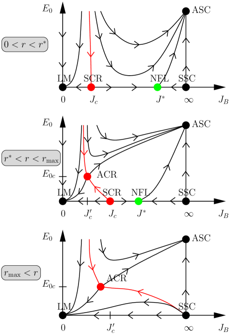
Figure 1: (color online) Renormalization group flow diagrams for the $S=1$ pseudogap Kondo model, deduced from NRG calculations ingersent . The horizontal axis is the Kondo coupling, the vertical axis denotes the amount of p-h symmetry breaking. Depending on the value of the bath exponent $r$, three distinct situations are found. The red lines represent phase boundaries, the red dots critical fixed points. For a detailed explanation of the fixed points see text.

Let us focus on the p-h symmetric case, $E_{0}=0$, first. At $J_{B}=0$ we have a free spin $1$, dubbed local-moment (LM) fixed point, which is stable w.r.t a small Kondo coupling $J_{B}$ for $r>0$. Flow towards large coupling is possible only when $J_{B}$ exceeds a critical value $J_{c}$ – this phase transition defines a symmetric critical (SCR) point. Contrary to the $S=1/2$ case where a symmetric strong-coupling (SSC) fixed point (corresponding to $J_{B}=\infty$) is always attained when $J_{B}>J_{c}$, SSC is generically unstable in the $S=1$ model, which instead shows an intermediate stable fixed point (NFL). It is located at a finite value $J^{*}>J_{c}$ and corresponds to a non-Fermi liquid (NFL) phase. This flow structure does not persist for all values of $r$, since at a value $r_{{\mathrm{max}}}\simeq 0.27$, the SCR and NFL fixed points collapse and disappear altogether. For $r>r_{{\mathrm{max}}}$, LM becomes then generically stable rmaxfoot .

Now we turn to finite p-h asymmetry, i.e., potential scattering $E_{0}\neq 0$. Then SCR is stable against finite $E_{0}$ only for $0<r<r^{*}$ (where $r^{*}\simeq 0.245$), whereas NFL is always unstable. In the case $r>r^{*}$, SCR becomes unstable as well, so that an asymmetric cousin of the critical point, ACR, exists and controls the quantum phase transition between LM and an asymmetric strong-coupling (ASC) fixed point. ACR is associated to finite values $J_{c}^{\prime}$ and $E_{0c}$ of both the Kondo coupling and the potential scattering term.

The numerical simulations of Ref. ingersent, have also established the behavior of several observables, such as the impurity contributions to the entropy and to the Curie susceptibility, for the various fixed points. Whereas the trivial cases (LM, SSC, ASC) are readily understood, all intermediate-coupling fixed points (SCR, NFL, ACR) correspond to fractional values of both the ground state degeneracy and spin, and cannot be understood on the basis of an independent electron picture. The values extracted from the Numerical Renormalization Group data are shown on Table I, and in the remainder of the paper we aim at an analytical calculation of such singular properties, which characterize the complicated nature of the various ground states occuring in the model.

Fixed point $(J,E_{0})$	Entropy	Curie constant
LM $(0,0)$	$\ln 3$	$2/3$
SCR $(J_{c},0)$	$\ln 3+ar^{3}$	$2/3-0.7r$
NFL $(J^{*},0)$	$\ln 2+2r\ln 2$	$1/4+0.4r$
SSC $(\infty,0)$	$\ln 2+2r\ln 2$	$1/4+r/8$
ACR $(J_{c}^{\prime},E_{0c})$	$1.6-0.7(1-r)$	$0.5-0.04(1-r)$
ASC $(\infty,\infty)$	$\ln 2$	$1/4$

Table 1: Numerical values of the impurity contribution to the entropy and to the Curie constant, for the various fixed points of the $S=1$ pseudogap Kondo model for $0\leq r\leq 1$, as determined by NRG ingersent . For LM, SSC, ASC the quoted values are exact.

IV Particle-hole symmetric model

In this section we analyze the particle-hole symmetric spin-1 pseudogap Kondo model (2), with $E_{0}=0$. We start with the weak-coupling RG which allows to capture the SCR fixed point for small $r$. Then we consider an expansion around the symmetric strong-coupling fixed point – this will lead us to an effective ferromagnetic Kondo model with singular density of states which we use to describe the physics of the stable NFL fixed point.

IV.1 Weak-coupling analysis of the SCR fixed point

The study of the regime with small Kondo coupling and particle-hole symmetry was done by Withoff and Fradkin fradkin for $S=1/2$. Perturbative RG is performed around $J_{B}=0$, i.e., the LM fixed point. The tree level scaling dimension of the Kondo coupling is ${\rm dim}[J_{B}]=-r$, and the RG flow in the vicinity of the LM fixed point can be described by the one-loop beta function:

$$\beta(j)=rj-j^{2}+{\mathcal{O}}(j^{3})$$ (3)

where $j$ is the renormalized dimensionless Kondo coupling, defined in Eq. 7 below. The beta function (3) obviously yields an unstable fixed point at $j_{c}=r$, which corresponds to SCR and controls the transition between LM and NFL. The correlation length exponent is

$$\frac{1}{\nu}=r+{\cal O}(r^{2})\,,$$ (4)

and $r=0$ can be interpreted as lower-critical “dimension” for the phase transition.

These results can be expected to persist for $S=1$, since the beta function for the Kondo problem is known fabrizio to be independent of the impurity spin value $S$. However, as we are interested in computing physical observables at SCR, which do differ from their $S=1/2$ counterparts, we will proceed with a complete RG analysis for $S=1$ as well. We only sketch here the intermediate results, while details on the derivation can be found in Appendix A.

IV.1.1 RG procedure

The analysis is based on a representation of the spin 1 by a triplet of Abrikosov fermions, $f_{mB}$:

$$S_{B}^{+} = S_{B}^{x}+iS_{B}^{y}=\sqrt{2}(f^{\dagger}_{1B}f^{\phantom{\dagger}}_{0B}+f^{\dagger}_{0B}f^{\phantom{\dagger}}_{-1B})\,,$$

$$S_{B}^{z} = f^{\dagger}_{1B}f^{\phantom{\dagger}}_{1B}-f^{\dagger}_{-1B}f^{\phantom{\dagger}}_{-1B}$$ (5)

where the Hilbert space constraint

$$Q=\sum_{m=1,0,-1}f^{\dagger}_{mB}f^{\phantom{\dagger}}_{mB}=1$$ (6)

is enforced kircan ; lambda using a chemical potential $\lambda\to\infty$.

To proceed with the RG scheme, we relate the bare coupling constant and field, $J_{B}$ and $f_{mB}$, to renormalized quantities, $j$ and $f_{m}$ (which bear no index to shorten the notation within renormalized perturbation theory):

$$N_{0}J_{B} = \mu^{-r}Z_{f}^{-1}Z_{J}j\,,$$ (7)

$$f_{mB} = Z_{f}^{1/2}f^{\phantom{\dagger}}_{m}$$ (8)

where $\mu$ is a renormalization energy scale. These equations define renormalization factors $Z_{J}$ and $Z_{f}$ which will be determined using the standard field-theoretic RG scheme bgz , employing dimensional regularization and minimal subtraction of poles.

A one-loop calculation (see Appendix A) of the $f^{\phantom{\dagger}}_{m}$ self-energy and the Kondo vertex yields

$$Z_{f} = 1+{\mathcal{O}}(j^{2})\,,$$ (9)

$$Z_{J} = 1+\frac{j}{r}+{\mathcal{O}}(j^{2})\,,$$ (10)

respectively. The RG beta function is obtained by the condition that the bare Kondo coupling is scale invariant, i.e. $dJ_{B}/d\mu=0$, which gives from (7):

$$\beta(j)\equiv\mu\frac{dj}{d\mu}=\frac{rj}{1+j\frac{d}{dj}\ln(Z_{J}/Z_{f})}\,.$$ (11)

Inserting (9)-(10) into this expression proves that the beta function in the $S=1$ case is still given by Eq. (3), as expected. We also note that p-h asymmetry is irrelevant at this fixed point, with $\beta(e_{0})=re_{0}$ (where $e_{0}\propto N_{0}E_{0}$ is the dimensionless potential scattering term).

IV.1.2 Impurity entropy

The impurity contribution to the entropy is obtained as the difference of the total entropy and the entropy of the electron bath alone. Its $T=0$ value represents a measure of the impurity ground state degeneracy. For the SCR fixed point it turns out that corrections to the LM value are extremely small kircan :

$$S_{{\mathrm{imp}}}^{{{\mathrm{SCR}}}}=\ln 3+{\mathcal{O}}(r^{3})~{}.$$ (12)

This makes the comparison to numerical data difficult, and we refrain from extracting the prefactor of the $r^{3}$ term.

IV.1.3 Impurity susceptibility

The impurity susceptibility $\chi_{{\mathrm{imp}}}$ is similarly calculated by removing the free (i.e. $J_{B}=0$) contribution of the bulk fermions to the total spin susceptibility suscfoot ,

$$\chi_{{\mathrm{tot}}}(T)=\int_{0}^{\beta}\!\!\!\!{{\mathrm{d}}}\tau\big{<}S^{z}_{{\mathrm{tot}}}(\tau)S^{z}_{{\mathrm{tot}}}(0)\big{>}\,,$$ (13)

with

$$S^{z}_{{\mathrm{tot}}}=\sum_{m}mf^{\dagger}_{mB}f^{\phantom{\dagger}}_{mB}+\sum_{{\bf x}\sigma}\frac{(-1)^{\sigma}}{2}c^{\dagger}_{\sigma}({\bf x})c^{\phantom{\dagger}}_{\sigma}({\bf x})\,.$$ (14)

Apart from numerical factors, the calculation is analogous to the $S=1/2$ case kircan , and we find at lowest order in $j$:

$$\chi_{{\mathrm{imp}}}=\frac{2}{3T}-j\frac{2}{3T}\left(\frac{\mu}{T}\right)^{-r}\int_{-\infty}^{+\infty}{{\mathrm{d}}}x\;\frac{e^{-x}}{(e^{-x}+1)^{2}}$$ (15)

Because we want to obtain the SCR fixed point contribution, we can replace $j=j_{c}=r$ and take $(\mu/T)^{-r}\simeq 1$ as $r\rightarrow 0$, which gives finally the effective Curie constant:

$$T\chi_{{\mathrm{imp}}}^{{\mathrm{SCR}}}=\frac{2}{3}-\frac{2r}{3}\,,$$ (16)

in agreement with the numerical value found in Table I.

IV.2 Non-Fermi liquid phase near strong coupling

IV.2.1 Around the limit $J=\infty$

To understand the emergence of a stable non-trivial fixed point, we consider in the first place the vicinity of the SSC fixed point. Indeed, the renormalization flow sketched from the numerical solution demonstrates that the strong-coupling fixed point is unstable, which is quite curious at first thought. Indeed, at large $J$, the spin 1 is partially screened by the fermions at site ${\bf 0}$, leaving a remnant effective spin $S_{{\mathrm{eff}}}=1/2$. Applying the Nozières-Blandin argument nozieres we see that an effective ferromagnetic coupling $J_{{\mathrm{eff}}}=-t_{01}^{2}/J$ is then generated between $\vec{S}_{{\mathrm{eff}}}$ and the electrons $c^{\dagger}_{\sigma}({\bf 1})$ sitting on the site near $c^{\dagger}_{\sigma}({\bf 0})$ (above, $t_{01}$ is the typical hopping between $c^{\dagger}_{\sigma}({\bf 0})$ and $c^{\dagger}_{\sigma}({\bf 1})$, and we assumed a chain representation of the electronic bath). Naively we would then expect SSC to be stable. This is not the case, because at particle-hole symmetry the Green’s functions of the above electrons are related through:

$$\big{<}c^{\dagger}_{\sigma}({\bf 0},i\omega)c^{\phantom{\dagger}}_{\sigma}({\bf 0},i\omega)\big{>}^{-1}=i\omega-t_{01}^{2}\big{<}c^{\dagger}_{\sigma}({\bf 1},i\omega)c^{\phantom{\dagger}}_{\sigma}({\bf 1},i\omega)\big{>}$$ (17)

which shows that the fermions $c^{\dagger}_{\sigma}({\bf 1})$ have an effective density of states $\rho_{{\mathrm{eff}}}(\epsilon)\propto|\epsilon|^{r_{{\mathrm{eff}}}}$, with $r_{{\mathrm{eff}}}=-r<0$.

Thus, the effective Hamiltonian near SSC is a ferromagnetic spin-1/2 Kondo model with a negative DOS exponent. Interestingly, this model was studied before in Ref. bulla, , and was found to display a stable intermediate-coupling fixed point. To see this, we note that the beta function for $J_{{\mathrm{eff}}}$ reads

$$\beta(j_{{\mathrm{eff}}})=r_{{\mathrm{eff}}}j_{{\mathrm{eff}}}-j_{{\mathrm{eff}}}^{2}=-rj_{{\mathrm{eff}}}-j_{{\mathrm{eff}}}^{2}\,.$$ (18)

This yields a stable fixed point at $j_{{\mathrm{eff}}}^{*}=-r$, which is allowed since the effective coupling is ferromagnetic! In our original language, this is the NFL fixed point, which controls now a whole phase with non-trivial properties, and is a unique feature of the $S>1/2$ pseudogap Kondo model. In particular, the above arguments show that this fixed point is located at $j^{*}\sim 1/r$. The NFL fixed point is unstable with respect to particle-hole asymmetry, with $\beta(e_{0})=-re_{0}$, a situation which will be discussed in Sec. V. Finally, we note that the values for $r^{*}$ and $r_{{\mathrm{max}}}$ obtained by the Numerical Renormalization Group for the original problem ingersent and for the effective model bulla coincide, in agreement with our identification. We would like now to compute the physical quantities at the intermediate NFL fixed point.

IV.2.2 Impurity entropy

We know that the correction to the entropy at a particle-hole symmetric Withoff-Fradkin type of fixed point is as small as $r^{3}$. However, we are now expanding around a strong-coupling fixed point and not with respect to a free spin $S=1$. Since the impurity entropy is defined relative to the decoupled ($J=0$) limit, we have to take into account the contribution at SSC ($J_{B}=\infty$), which contains a $\ln 2$ term due to the underscreened spin $S_{{\mathrm{eff}}}=1/2$, and depends on $r$ as well ingersent ; fritz1 , due to the singular nature of the resonant level limit (although the SSC fixed point is trivial). We obtain finally

$$S_{{\mathrm{imp}}}^{{\mathrm{NFL}}}=\ln 2+2r\ln 2+{\mathcal{O}}(r^{3})\,,$$ (19)

as anticipated numerically (Table I).

IV.2.3 Impurity susceptibility

We have to follow the same argument as above, and sum the contribution of the strong-coupling fixed point, $T\chi_{{\mathrm{imp}}}^{{\mathrm{SSC}}}=1/4+r/8$ (see fritz1 ) as well as the non-trivial correction due to the stable $S_{{\mathrm{eff}}}=1/2$ ferromagnetic fixed point with exponent $r_{{\mathrm{eff}}}=-r$, which is kircan $\Delta(T\chi_{{\mathrm{imp}}})=-r_{{\mathrm{eff}}}/4=r/4$. The complete result thus agrees with the value in Table I:

$$T\chi_{{\mathrm{imp}}}^{{\mathrm{NFL}}}=\frac{1}{4}+\frac{3r}{8}\,.$$ (20)

V Particle-hole asymmetric model

The nature of the particle-hole asymmetric fixed point of the pseudogap Kondo model, present at $E_{0}\neq 0$ and $r>r^{*}$, was understood in the recent work fritz1 ; fritz2 . The crucial point noticed there is that this quantum phase transition separates the local-moment fixed point from the asymmetric strong-coupling one, as can be checked in Fig. 1, so that the corresponding field theory can be constructed by “mixing” the relevant degrees of freedom associated to both fixed points. In the $S=1/2$ case, one needed to consider a level crossing of a doublet (associated to LM) and a singlet (from to ASC), with transitions allowed through the coupling to the conduction electrons. Not surprisingly, the effective theory took the form of an infinite-$U$, i.e., maximally p-h asymmetric, Anderson model. This was perfectly consistent with numerical data which indicate the phase transitions in the pseudogap Kondo and Anderson models are in the same universality class. The theory could be analyzed by expanding around the level-crossing (valence fluctuation) fixed point, and it was shown that $r=1$ plays the role of an upper-critical “dimension”.

In the following, we want to generalize the idea of Refs. fritz1, ; fritz2, to the spin-1 case.

V.1 Derivation of the critical field theory

In the present problem, the spin $S=1$ will be described by a triplet of fermions $f^{\phantom{\dagger}}_{m}$ near LM. On the other hand, ASC shows underscreening of the spin, and gives a remnant spin-1/2 moment, that we can describe by a doublet of bosons $b^{\phantom{\dagger}}_{\sigma}$. Having now the important variables to describe the transition at ACR, we need to write down the effective theory. Several requirements have to be imposed: the Hamiltonian should obey spin rotation invariance and should reduce to a spin 1 (resp. 1/2) Kondo Hamiltonian near the LM (resp. ASC) limit. One naturally arrives at the following generalization of the infinite-$U$ Anderson model of Ref. fritz1, :

$${\cal H} = \sum_{k\sigma}\epsilon_{k}c^{\dagger}_{k\sigma}c^{\phantom{\dagger}}_{k\sigma}+\epsilon_{f}\sum_{m}f^{\dagger}_{m}f^{\phantom{\dagger}}_{m}$$

$$+ V_{B}\big{[}f^{\dagger}_{0B}b^{\phantom{\dagger}}_{\downarrow B}\,c^{\phantom{\dagger}}_{\uparrow}({\bf 0})+f^{\dagger}_{0B}b^{\phantom{\dagger}}_{\uparrow B}\,c^{\phantom{\dagger}}_{\downarrow}({\bf 0})\big{]}+{{\mathrm{h.c.}}}$$

$$+ \sqrt{2}V_{B}\big{[}f^{\dagger}_{1B}b^{\phantom{\dagger}}_{\uparrow B}\,c^{\phantom{\dagger}}_{\uparrow}({\bf 0})+f^{\dagger}_{-1B}b^{\phantom{\dagger}}_{\downarrow B}\,c^{\phantom{\dagger}}_{\downarrow}({\bf 0})\big{]}+{{\mathrm{h.c.}}}\,.$$

Here, $\epsilon_{f}$ is the parameter used to tune the system through the phase transition; at tree level the transition occurs at $\epsilon_{f}=0$, and corresponds to the crossing of doublet and triplet states, which we call the valence fluctuation (VFl) fixed point. The restriction to the physical Hilbert space is implemented with the constraint

$$Q=\sum_{m}f^{\dagger}_{mB}f^{\phantom{\dagger}}_{mB}+\sum_{\sigma}b^{\dagger}_{\sigma B}b^{\phantom{\dagger}}_{\sigma B}=1\,.$$ (22)

One can check easily via a Schrieffer-Wolff transformation that ${\cal H}$ (V.1) evolves onto a spin 1 (resp. 1/2) Kondo model when $\epsilon_{f}$ is large and negative (resp. positive), as it should be.

The effective Hamiltonian (V.1) seems to have nothing to do with the original model (2), and in particular it is not as simply understandable as in the $S=1/2$ case considered in fritz2 . However, we will show that it correctly describes the critical properties at ACR. A number of facts are encouraging: Power counting at the $\epsilon_{f}=V_{B}=0$ fixed point shows that the coupling constant $V_{B}$ has a tree-level scaling dimension ${\rm dim}[V_{B}]=\bar{r}=(1-r)/2$, i.e., it is relevant for $r<1$, which indicates the possibility of a non-trivial critical point in this regime. In contrast, $V_{B}$ is irrelevant and will flow to zero for $r>1$, which establishes the role of $r=1$ as upper-critical dimension where $V_{B}$ is marginal. Similar to the situation in the spin-1/2 model, the transition will become a level crossing with perturbative corrections for $r>1$. For $V_{B}\to 0$ we have strong “valence” fluctuations between the doublet and triplet levels, leading to an entropy of $\ln 5$, in agreement with the numerical result shown in Table I.

Motivated by this we proceed with an RG expansion around the decoupled $V_{B}=0$ fixed point. As demonstrated below, we find a flow diagram identical in structure to the one of the spin-1/2 model, Fig. 1 of Ref. fritz2, , with the difference that the VFl fixed point now corresponds to a crossing of doublet and triplet levels. This flow diagram is very similar to the one of a standard $\phi^{4}$ theory. In particular, the non-trivial critical point occuring for $r<1$ (which can be understood as the analogue of the Wilson-Fisher fixed point) will be identified with the asymmetric critical point (ACR) of the original Kondo Hamiltonian.

V.2 RG calculation for $r$ close to 1

V.2.1 RG procedure

The renormalization method developed in Ref. fritz2, differs slightly from the technique used in Sec. IV.1 and Appendix A. We still need to introduce renormalization factors for the hybridization strength and fields:

$$N_{0}V_{B} = \mu^{+\bar{r}}Z_{f}^{-1/2}Z_{b}^{-1/2}Z_{V}v\,,$$ (23)

$$f_{mB} = Z_{f}^{1/2}f^{\phantom{\dagger}}_{m}\,,$$ (24)

$$b_{\sigma B} = Z_{b}^{1/2}b^{\phantom{\dagger}}_{\sigma}\,,$$ (25)

as well as mass renormalization terms,

$${\cal H}_{\lambda}=\delta\lambda_{f}\sum_{m}f^{\dagger}_{m}f^{\phantom{\dagger}}_{m}+\delta\lambda_{b}\sum_{\sigma}b^{\dagger}_{\sigma}b^{\phantom{\dagger}}_{\sigma}\,,$$ (26)

already written using renormalized quantities. We have introduced again a running renormalization scale $\mu$ and used $\bar{r}=(1-r)/2$.

The RG will be performed at criticality, i.e., the $\delta\lambda$ are chosen such to cancel the real parts of the bare self-energies. Including the contribution of the counter-terms associated to the above renormalization constants, we find (see Appendix B) the $f$-electron self-energy contribution at one-loop:

$$\Sigma_{f}(i\omega)=-2v^{2}\left(\frac{\mu}{D}\right)^{\bar{r}}\!\!\left[D\!+\!\frac{i\omega}{2\bar{r}}\left(\frac{D}{|\omega|}\right)^{\bar{r}}\right]+\delta\lambda_{f}-i\omega(Z_{f}-1)\,.$$ (27)

By definition, the field renormalization is determined by the condition $(\partial/\partial\omega)\Sigma_{f}(0)=0$, and criticality is ensured by the vanishing of the mass, $\Sigma_{f}(0)=0$, which gives:

$$Z_{f} = 1-\frac{v^{2}}{\bar{r}}+{\mathcal{O}}(v^{4})\,,$$ (28)

$$\delta\lambda_{f} = 2v^{2}\left(\frac{\mu}{D}\right)^{\bar{r}}D+{\mathcal{O}}(v^{2})\,.$$ (29)

The bosonic self-energy is similarly calculated (only numerical prefactors differ) and leads to:

$$Z_{b} = 1-\frac{3v^{2}}{2\bar{r}}+{\mathcal{O}}(v^{4})\,,$$ (30)

$$\delta\lambda_{b} = 3v^{2}\left(\frac{\mu}{D}\right)^{\bar{r}}D+{\mathcal{O}}(v^{2})\,.$$ (31)

At this order, the hybridization is left unrenormalized, $Z_{V}=1$. Finally, imposing the scale invariance condition ${{\mathrm{d}}}V_{B}/{{\mathrm{d}}}\mu=0$, we find the beta function:

$$\beta(v) \equiv \mu\frac{{{\mathrm{d}}}v}{{{\mathrm{d}}}\mu}=\frac{-\bar{r}v}{1+v\frac{d}{dv}\ln(Z_{V}Z_{f}^{-1/2}Z_{b}^{-1/2})}$$ (32)

$$= -\bar{r}v+\frac{5}{2}v^{3}+{\mathcal{O}}(v^{5}).$$

This gives the fixed point value $(v^{*})^{2}=(2/5)\bar{r}$. The correlation length exponent of the LM–ASC transition can be obtained similar to Ref. fritz2, , with the result

$$\frac{1}{\nu}=r+{\cal O}(\bar{r}^{2})~{}~{}~{}~{}(r<1)\,,$$ (33)

whereas a level crossing (formally $\nu=1$) occurs for $r>1$. The RG flow is thus identical to Fig. 1 of Ref. fritz2, .

V.2.2 Impurity entropy

The correction at order $v^{2}$ to the free energy is evaluated in Appendix B and reads:

$$\Delta F=-\frac{12}{5}v^{2}\mu^{2\bar{r}}\int_{0}^{D}{{\mathrm{d}}}\epsilon\;\frac{\epsilon^{r}}{\epsilon}\;\tanh\frac{\epsilon}{2T}$$ (34)

Using $\Delta S_{{\mathrm{imp}}}=-\partial(\Delta F)/\partial T$, and taking the limit $\bar{r}\rightarrow 0$, we obtain finally:

$$S_{{\mathrm{imp}}}^{{\mathrm{ACR}}}=\ln 5-\frac{24\ln 2}{25}(1-r)$$ (35)

which is a agreement with the result in Table I.

V.2.3 Impurity susceptibility

The computation of the Curie constant is done along the same line, but is more involved due to the proliferation of Feynman graphs, since the total spin operator

$$S^{z}_{{\mathrm{tot}}} = \sum_{m}mf^{\dagger}_{mB}f^{\phantom{\dagger}}_{mB}$$ (36)

$$+ \sum_{\sigma}\frac{(-1)^{\sigma}}{2}\left[b^{\dagger}_{\sigma B}b^{\phantom{\dagger}}_{\sigma B}+\sum_{\bf x}c^{\dagger}_{\sigma}({\bf x})c^{\phantom{\dagger}}_{\sigma}({\bf x})\right]$$

mixes all three possible fields in the calculation. We simply quote the final result, derived in Appendix B:

$$\chi_{{\mathrm{imp}}} = \frac{1}{2T}-\frac{v^{2}\mu^{2\bar{r}}}{10T}\int_{0}^{D}{{\mathrm{d}}}\epsilon\;\frac{\epsilon^{r}}{T^{2}}\;\left[\frac{\sinh\epsilon/T}{1+\cosh\epsilon/T}-1\right.$$ (37)

$$\left.+\frac{6\sinh\epsilon/T}{(1+\cosh\epsilon/T)^{2}}\right].$$

We finally insert the fixed-point value $v^{*}$ and take the limit $\bar{r}\rightarrow 0$, which gives:

$$T\chi_{{\mathrm{imp}}}^{{\mathrm{SCR}}}=\frac{1}{2}-\frac{3-2\ln 2}{50}(1-r)\,.$$ (38)

Note that the leading Curie constant above is associated to the trivial susceptibility of a magnetic system that consists of a triplet and a singlet. Because of numerical prefactors, e.g. in the partition function, it is not simply given by the expression valid for a triplet state only, namely S(S+1)/3=2/3, but by the different value 1/2. Finally, we check that equation (38) coincides with the results in Table I and vindicates the usefulness of the effective theory (V.1) in describing the ACR fixed point.

VI Conclusion

In this paper, we have studied the spin-1 pseudogap Kondo model using perturbative RG together with renormalized perturbation theory. We have shown that all non-trivial fixed points are accessible in the vicinity of their associated upper-critical or lower-critical dimension. In particular, we have proposed a novel field theory governing the critical behavior in the presence of particle-hole asymmetry, and we also have provided a physical picture for the stable particle-hole symmetric non-Fermi liquid phase (which is not present in the $S=1/2$ case) using a strong-coupling mapping to an effective ferromagnetic spin-1/2 model with singular density of states. The generic instability of the symmetric strong-coupling fixed point SSC and the emergence of the non-Fermi liquid phase presents a nice example of a situation where the purely local strong-coupling picture of Kondo singlet formation is clearly inappropriate. We also note that, from the arguments given above, our qualitative results are expected to be generic to the pseudogap Kondo model for all spin values $S$ greater or equal to 1.

The collected analytical results for thermodynamic quantities established in this paper can finally be compared to the numerical values obtained from the simulations ingersent , and are displayed in Fig. 2 and 3. The agreement is excellent, even at one-loop order, demonstrating the usefulness of $\epsilon$-expansions for impurity models with power-law bath spectra.

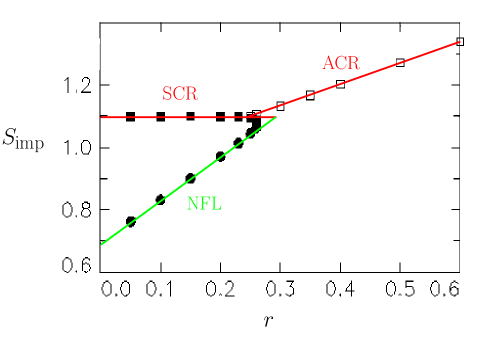
Figure 2: (color online) Comparison of the impurity entropy $S_{\rm imp}$ between the analytical estimates at one-loop order (continuous lines) and the NRG data of Ref. ingersent, (dots and squares) for the three different intermediate-coupling fixed points occuring in the $S=1$ pseudogap Kondo model.

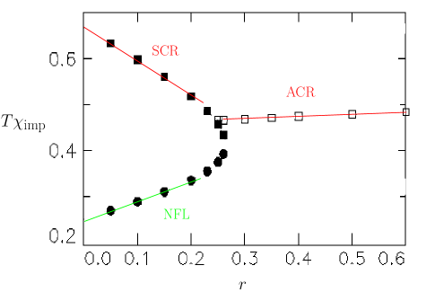
Figure 3: (color online) As Fig. 2, but for the effective Curie constant $T\chi_{\rm imp}$.

Using the present RG methods other observables can be calculated as well fritz2 , like the critical exponents for the local susceptibility or the conduction electron $T$ matrix. We only mention here the result for the $T$ matrix: similar to the spin-1/2 model the critical exponent can be determined exactly to all orders in perturbation theory, with the result

$${\rm Im}\,T(\omega)\propto\frac{1}{\omega^{r}}~{}~{}~{}(0<r<1)$$ (39)

which holds at all intermediate coupling fixed points (SCR, NFL, ACR). At the critical dimensions, $r=0$ and $r=1$, logarithmic corrections to this result occur.

The application of our results to experiments requires host systems with pseudogap DOS. Candidates are $d$-wave superconductors or materials with a special semiconducting band structure (as planar graphite) – these obey a linearly vanishing density of states. Systems with exponent $0<r<1$ are difficult to realize; proposals have been made e.g. using disordered mesoscopic conductors hopk .

On the theoretical side, the single-impurity pseudogap Kondo problems are now reasonably well understood. One open issue is a possible analytical description of a collapse of intermediate-coupling fixed points, which occurs both as $r\to{r^{*}}^{+}$ (where two critical fixed points merge) and at $r\to{r_{{\mathrm{max}}}}^{-}$ (where the stable and the critical p-h symmetric fixed points meet and disappear). One idea comes to mind when comparing the entropies for a spin-$S$ model: the critical fixed point has $S_{{\mathrm{imp}}}(J_{c})=\ln(2S+1)+{\mathcal{O}}(r^{3})$, whereas for the stable NFL fixed point has $S_{{\mathrm{imp}}}(J^{*})=\ln(2S)+2r\ln 2+{\mathcal{O}}(r^{3})$. The two values cross at $r_{{\mathrm{max}}}\sim 1/(S\ln 8)$, a value that becomes small if $S\gg 1$. One may hope that a controlled weak-coupling theory describing the physics of $r_{{\mathrm{max}}}$ or $r^{\ast}$ exists for large $S$, although this remains to be demonstrated. Finally, we point out that generalizations of the pseudogap model to several impurities can show an interesting interplay of critical points with different nature.

Appendix A Weak-coupling RG

Here we provide calculational details for the weak-coupling RG of Sec. IV.1.

A.1 Vertex renormalization at one loop

We first rewrite the bare Kondo Hamiltonian (2) in terms of renormalized quantities, allowing to separate the bare action ${\mathcal{S}}_{B}$ into a renormalized Kondo part ${\mathcal{S}}$, a constraint term ${\mathcal{S}}_{\lambda}$, and a series of counter-terms $\delta{\mathcal{S}}$:

$${\mathcal{S}}_{B} = {\mathcal{S}}+{\mathcal{S}}_{\lambda}+\delta{\mathcal{S}}\,,$$ (40)

$${\mathcal{S}} = \int_{0}^{\beta}\!\!\!\!{{\mathrm{d}}}\tau\sum_{k}{\bar{c}}^{\phantom{\dagger}}_{k\sigma}(\partial_{\tau}+\epsilon_{k})c^{\phantom{\dagger}}_{k\sigma}+\sum_{m}{\bar{f}}^{\phantom{\dagger}}_{m}\partial_{\tau}f^{\phantom{\dagger}}_{m}$$ (41)

$$+\int_{0}^{\beta}\!\!\!\!{{\mathrm{d}}}\tau\!\!\sum_{mm^{\prime}\sigma\sigma^{\prime}}\Gamma_{mm^{\prime}\sigma\sigma^{\prime}}^{(0)}{\bar{f}}^{\phantom{\dagger}}_{m}f^{\phantom{\dagger}}_{m}{\bar{c}}^{\phantom{\dagger}}_{\sigma}({\bf 0})c^{\phantom{\dagger}}_{\sigma}({\bf 0})\,,$$

$${\mathcal{S}}_{\lambda} = \int_{0}^{\beta}\!\!\!\!{{\mathrm{d}}}\tau\;\lambda\bigg{(}\sum_{m}{\bar{f}}^{\phantom{\dagger}}_{m}f^{\phantom{\dagger}}_{m}-1\bigg{)}\,,$$ (42)

$$\delta{\mathcal{S}} = \int_{0}^{\beta}\!\!\!\!{{\mathrm{d}}}\tau\;\delta\lambda\sum_{m}{\bar{f}}^{\phantom{\dagger}}_{m}f^{\phantom{\dagger}}_{m}$$

$$+\int_{0}^{\beta}\!\!\!\!{{\mathrm{d}}}\tau\;(Z_{J}-1)\!\!\sum_{mm^{\prime}\sigma\sigma^{\prime}}\Gamma_{mm^{\prime}\sigma\sigma^{\prime}}^{(0)}{\bar{f}}^{\phantom{\dagger}}_{m}f^{\phantom{\dagger}}_{m}{\bar{c}}^{\phantom{\dagger}}_{\sigma}({\bf 0})c^{\phantom{\dagger}}_{\sigma}({\bf 0})\,.$$

With a renormalized dimensionful coupling $J=j/N_{0}$ the tree level vertices satisfy $\Gamma_{10\downarrow\uparrow}^{(0)}=\Gamma_{0-1\downarrow\uparrow}^{(0)}=\Gamma_{01\uparrow\downarrow}^{(0)}=\Gamma_{-10\uparrow\downarrow}^{(0)}=\mu^{-r}J/\sqrt{2}$ and $\Gamma_{mm\sigma\sigma}^{(0)}=\mu^{-r}Jm(-1)^{\sigma}/2$, with all other terms being zero. Indeed, inserting the definitions (7)-(8) into the above expression for the action, one recovers the bare action of the problem. The free propagators are given by:

$$G_{c0}(i\omega,k) = \frac{1}{i\omega-\epsilon_{k}}$$ (44)

$$G_{f0}(i\omega) = \frac{1}{i\omega-\lambda}$$ (45)

where the limit $\lambda\rightarrow\infty$ should be taken only at the end of the calculation lambda . The diagrammatic expansion at one loop of the vertex $\Gamma_{10\downarrow\uparrow}$ is given in Fig. 4.

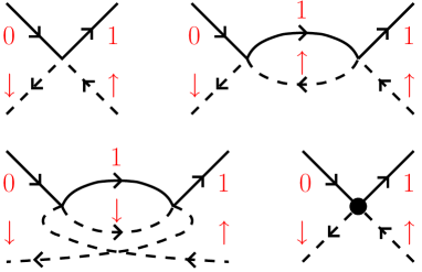
Figure 4: (color online). Renormalization of the vertex $\Gamma_{10\downarrow\uparrow}^{(1)}$ at one-loop level. Continuous and dashed lines denote the free Green’s functions of the $f_{m}$ and $c_{\sigma}$ fields respectively, and the dot represents the vertex counter-term $(Z_{J}-1)\Gamma_{10\downarrow\uparrow}^{(0)}$.

Evaluating the loop at zero temperature, one finds:

$$\Gamma_{10\downarrow\uparrow}^{(1)}(i\nu) = \mu^{-r}Z_{J}\frac{J}{\sqrt{2}}-\mu^{-2r}\frac{J^{2}}{\sqrt{2}}\int_{-D}^{0}{{\mathrm{d}}}\epsilon\;N_{0}\frac{|\epsilon|^{r}}{\epsilon+i\nu}$$ (46)

$$= \frac{J}{\sqrt{2}}\mu^{-r}\left[Z_{J}-\frac{j}{r}(1+r\ln\big{(}|\nu|/\mu)\big{)}\right]$$

where we have used $j=N_{0}J$, and the limit $r\rightarrow 0$ has been taken in the last integral. The renormalization condition for the vertex is $\Gamma_{10\downarrow\uparrow}^{(1)}(0)=\Gamma_{10\downarrow\uparrow}^{(0)}=\mu^{-r}J/\sqrt{2}$, so that the result (10) follows.

A.2 Impurity susceptibility

The diagrammatic expansion of the impurity susceptibility follows from its definition (13-14), and accounting for all numerical prefactors (which arise either from the $(-1)^{\sigma}/2$ term in (14) or from combinatorial reasons), we have to calculate the contribution shown in Fig. 5. Note that $\big{<}Q\big{>}\chi_{{\mathrm{imp}}}$ and not $\chi_{{\mathrm{imp}}}$ has a simple diagrammatic expansion, since the constraint $Q=\sum_{m}f^{\dagger}_{mB}f^{\phantom{\dagger}}_{mB}=1$ means that we are not expanding around a free-particle limit. At lowest order, we have $\big{<}Q\big{>}=3\exp(-\beta\lambda)$. Computing the Matsubara sums at finite temperature, one gets the result (15) in the limit where the half-bandwidth $D$ goes to infinity.

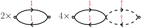
Figure 5: (color online). Diagrammatic expansion of $\big{<}Q\big{>}\chi_{{\mathrm{imp}}}$ at lowest order for the Kondo model at SCR, including the complete prefactors.

Appendix B RG around the valence-fluctuation limit

This appendix contains details for the RG calculation of Sec. V.2.

B.1 Pseudoparticle self-energies at one loop

Again, we will set up notations and express the bare action ${\mathcal{S}}_{B}={\mathcal{S}}+{\mathcal{S}}_{\lambda}+\delta{\mathcal{S}}$ in terms of renormalized quantities:

$${\mathcal{S}} = \int_{0}^{\beta}\!\!\!\!{{\mathrm{d}}}\tau\sum_{k\sigma}{\bar{c}}^{\phantom{\dagger}}_{k\sigma}(\partial_{\tau}+\epsilon_{k})c^{\phantom{\dagger}}_{k\sigma}$$

$$+\int_{0}^{\beta}\!\!\!\!{{\mathrm{d}}}\tau\sum_{m}{\bar{f}}^{\phantom{\dagger}}_{m}(\partial_{\tau}+\epsilon_{f})f^{\phantom{\dagger}}_{m}+\sum_{\sigma}{\bar{b}}^{\phantom{\dagger}}_{\sigma}\partial_{\tau}b^{\phantom{\dagger}}_{\sigma}$$

$$+\int_{0}^{\beta}\!\!\!\!{{\mathrm{d}}}\tau V\mu^{\bar{r}}\big{[}{\bar{f}}_{0}b^{\phantom{\dagger}}_{\downarrow}c^{\phantom{\dagger}}_{\uparrow}({\bf 0})+{\bar{f}}_{0}b^{\phantom{\dagger}}_{\uparrow}c^{\phantom{\dagger}}_{\downarrow}({\bf 0})\big{]}+{{\mathrm{c.c.}}}\,,$$

$$+\int_{0}^{\beta}\!\!\!\!{{\mathrm{d}}}\tau\sqrt{2}V\mu^{\bar{r}}\big{[}{\bar{f}}_{1}b^{\phantom{\dagger}}_{\uparrow}c^{\phantom{\dagger}}_{\uparrow}({\bf 0})+{\bar{f}}_{-1}b^{\phantom{\dagger}}_{\downarrow}c^{\phantom{\dagger}}_{\downarrow}({\bf 0})\big{]}+{{\mathrm{c.c.}}}\,,$$

$${\mathcal{S}}_{\lambda} = \int_{0}^{\beta}\!\!\!\!{{\mathrm{d}}}\tau\;\lambda\bigg{(}\sum_{m}{\bar{f}}^{\phantom{\dagger}}_{m}f^{\phantom{\dagger}}_{m}+\sum_{\sigma}{\bar{b}}^{\phantom{\dagger}}_{\sigma}b^{\phantom{\dagger}}_{\sigma}-1\bigg{)}\,,$$ (48)

$$\delta{\mathcal{S}} = \int_{0}^{\beta}\!\!\!\!{{\mathrm{d}}}\tau\;\delta\lambda_{f}\sum_{m}{\bar{f}}^{\phantom{\dagger}}_{m}f^{\phantom{\dagger}}_{m}+\delta\lambda_{b}\sum_{\sigma}{\bar{b}}^{\phantom{\dagger}}_{\sigma}b^{\phantom{\dagger}}_{\sigma}+\ldots$$ (49)

As above, we have introduced a renormalized dimensionful hybridization $V=v/N_{0}$. We did not write the vertex renormalization factor, since it will not appear at this order of the calculation. We also have to introduce the bosonic Green’s function :

$$G_{b0}(i\nu)=-\big{<}b^{\dagger}_{\sigma}(i\nu)b^{\phantom{\dagger}}_{\sigma}(i\nu)\big{>}=\frac{1}{i\nu-\lambda}\,.$$ (50)

Calculating the self-energy for the $f_{1}$ fermion shown in Fig. 6, we find at zero temperature:

$$\Sigma_{f}(i\omega)=-2N_{0}V^{2}\mu^{2\bar{r}}\int_{0}^{D}{{\mathrm{d}}}\epsilon\frac{\epsilon^{r}}{\epsilon-i\omega}+\delta\lambda_{f}-i\omega(Z_{f}-1)$$ (51)

which reduces to (27) when the limit $\bar{r}\rightarrow 0$ is taken. The calculation for the $b_{\uparrow}$ proceeds along the same line, although the prefactors differ slightly (see Fig. 6).

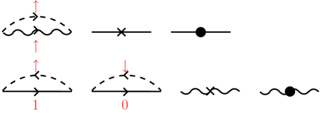
Figure 6: (color online). Self-energy at one loop for the $f_{1}$ fermion (upper part) and $b_{\uparrow}$ boson (lower part) respectively. Wiggly lines represent the bosonic free propagators. Crosses and dots indicate respectively mass and field renormalization counter-terms.

B.2 Impurity entropy

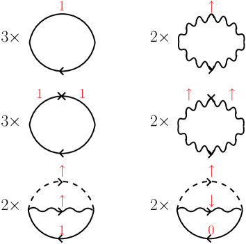
Figure 7: (color online). Expansion of the partition function ${\mathcal{Z}}$ up to order $V^{2}$ and $\delta\lambda_{f,b}$, including the combinatorial factors.

To evaluate the impurity entropy, we need to expand the physical partition function ${\mathcal{Z}}$, which is represented diagrammatically in Fig. 7. The free energy can then be obtained through $F=-T\ln{\mathcal{Z}}$, and reads:

$$F = -T\ln 5+\frac{12}{5}v^{2}\mu^{2\bar{r}}\int_{0}^{D}{{\mathrm{d}}}\epsilon\;\frac{\epsilon^{r}}{\epsilon}$$ (52)

$$-\frac{12}{5}v^{2}\mu^{2\bar{r}}\int_{0}^{D}{{\mathrm{d}}}\epsilon\;\frac{\epsilon^{r}}{\epsilon}\;\tanh\frac{\epsilon}{2T}$$

which is the result quoted in Eq. (34) from which the impurity entropy at the ACR fixed point follows. In deriving this result we have used the renormalized values for the counter-terms (29)-(31), which provide the correction in the first line of the above expresion. One can check that they actually drop out when the entropy is calculated, but those corrections are nevertheless crucial for regularizing the forthcoming impurity susceptibility.

B.3 Impurity susceptibility

Computing the impurity susceptibility is quite cumbersome, since many graphs appear at intermediate stages of the calculation, due to the fact that both pseudoparticles now carry a spin index. First, we recall that the quantity which admits a simple diagrammatics is in fact $\big{<}Q\big{>}\chi_{{\mathrm{imp}}}$ rather than $\chi_{{\mathrm{imp}}}$, where $\big{<}Q\big{>}$ is obtained from $\big{<}Q\big{>}=e^{-\beta\lambda}{\mathcal{Z}}$ and the above result for the free energy, Eq. (52). Again, we simply quote the collection of graphs that need to be evaluated in Fig. 8 (with the corresponding prefactor), and refer the reader to Ref. fritz1, for more details.

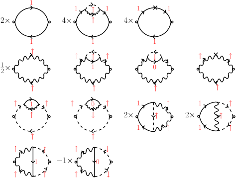
Figure 8: (color online). Diagrammatic expansion of $\big{<}Q\big{>}\chi_{{\mathrm{imp}}}$ at lowest order for the effective theory describing ACR, including the complete prefactors.

References

- (1) A. C. Hewson, The Kondo Problem to Heavy Fermions, Cambridge University Press, Cambridge (1996).
- (2) M. Vojta, cond-mat/0412208.
- (3) D. Withoff and E. Fradkin, Phys. Rev. Lett. 64, 1835 (1990).
- (4) L. Fritz and M. Vojta, Phys. Rev. B 70, 214427 (2004).
- (5) C. Gonzalez-Buxton and K. Ingersent, Phys. Rev. B 57, 14254 (1998).
- (6) M. Vojta and L. Fritz, Phys. Rev. B 70, 094502 (2004).
- (7) P. Mehta, L. Borda, G. Zarand, N. Andrei, and P. Coleman, cond-mat/0404122.
- (8) A. Posazhennikova and P. Coleman, Phys. Rev. Lett. 94, 036802 (2005).
- (9) corresponds here to the deviation of the parameter from its value at the lower-critical or upper-critical dimension.
- (10) Note that for , the value corresponds rather to the collapse of SCR and SSC. The critical point can then be captured by an expansion around SSC for close to as shown in Ref. fritz1, , which is not possible here since the collapse occurs at intermediate coupling.
- (11) M. Fabrizio and G. Zarand, Phys. Rev. B 54, 10008 (1996).
- (12) M. Kirćan and M. Vojta, Phys. Rev. B 69, 174421 (2004).
- (13) A. Zawadowski and P. Fazekas, Z. Physik 226, 235 (1969); P. Coleman, Phys. Rev. B 29, 3035 (1984).
- (14) E. Brezin, J. C. Le Guillou, and J. Zinn-Justin, in Phase transitions and critical phenomena, eds. C. Domb and M. S. Green, Page Bros., Norwich (1996), Vol. 6.
- (15) P. Nozières and A. Blandin, J. Physique 41, 193 (1980).
- (16) M. Vojta and R. Bulla, Eur. Phys. J. B 28, 283 (2002).
- (17) We define the spin susceptibility with respect to its component only due to spin rotation symmetry. For a free spin , we then have .
- (18) J. Hopkinson, K. Le Hur, and E. Dupont, cond-mat/0407165.