Odd Triplet Superconductivity and Related Phenomena in Superconductor-Ferromagnet Structures

Abstract

We consider novel unusual effects in superconductor-ferromagnet (S/F) structures. In particular we analyze the triplet component (TC) of the condensate generated in those systems.This component is odd in frequency and even in the momentum, which makes it insensitive to non-magnetic impurities. If the exchange field is not homogeneous in the system the triplet component is not destroyed even by a strong exchange field and can penetrate the ferromagnet over long distances. Some other effects considered here and caused by the proximity effect are: enhancement of the Josephson current due to the presence of the ferromagnet, induction of a magnetic moment in superconductors resulting in a screening of the magnetic moment, formation of periodic magnetic structures due to the influence of the superconductor, etc. We compare the theoretical predictions with existing experiments.

I Introduction

Although superconductivity has been discovered by H. Kammerlingh Onnes almost one century ago (1911), the interest in studying this phenomenon is far from declining. The great attention to superconductivity within the last 15 years is partly due to the discovery of the high temperature superconductors (HTSC) Bednorz and Müller (1986), which promises important technological applications. It is clear that issues such as the origin of the high critical temperature superconductivity, effects of external fields and impurities on HTCS, etc, will remain fields of interest for years to come.

Due to the successful investigations of the HTSC and its possible technological applications, the interest in studying properties of traditional (low $T_{c}$) superconductors was not as broad. Nevertheless this field has also undergone a tremendous development. Technologically, the traditional superconductors are often easier to manipulate than high $T_{c}$ cuprates. One of the main achievements of the last decade is the making of high quality contacts between superconductors and normal metals $(S/N)$, superconductors and ferromagnets $(S/F)$, superconductors and insulators $(S/I)$, etc. All these heterostructures can be very small with the characteristic sizes of submicrometers.

This has opened a new field of research. The small size of these structures provides the coherence of superconducting correlations over the full length of the $N$ region. The length of the condensate penetration into the $N$ region $\xi_{N}$ is restricted by decoherence processes (inelastic or spin-flip scattering). At low temperatures the characteristic length over which these decoherence processes occur may be quite long (a few microns). Superconducting coherent effects in $S/N$ nanostructures, such as conductance oscillations in an external magnetic field, were studied intensively during the last decade (see for example the review articles by Beenakker (1997); Lambert and Raimondi (1998)).

The interplay between a superconductor $(S)$ and a normal metal $(N)$ in simpler types of $S/N$ structures (for example, $S/N$ bilayers) has been under study for a long time and the main physics of this so called proximity effect is well described in the review articles by de Gennes (1964) and Deutscher and de Gennes (1969). In these works it was noticed that not only the superconductor changes the properties of the normal metal but also the normal metal has a strong effect on the superconductor. It was shown that near the $S/N$ interface the superconductivity is suppressed over the correlation length $\xi_{S}$, which means that the order parameter $\Delta$ is reduced at the interface in comparison with its bulk value far away from the interface. At the same time, the superconducting condensate penetrates the normal metal over the length $\xi_{N}$, which at low temperatures may be much larger than $\xi_{S}$. Due to the penetration of the condensate into the normal metal over large distances the Josephson effect is possible in $S/N/S$ junctions with the thicknesses of the $N$ regions of the order of a few hundreds nanometers. The Josephson effects in $S/N/S$ junctions were studied in many papers and a good overview, both experimental and theoretical, is given by Kulik and Yanson. (1970), Likharev (1979), and Barone and Paterno (1982).

The situation described above is quite different if an insulating layer $I$ is placed between two superconductors. The thickness of the insulator in $S/I/S$ structures cannot be as large as of the normal metals because electron wave functions decay in the insulator on atomic distances. As a consequence, the Josephson current is extremely small in $S/I/S$ structures with a thick insulating layer.

But what about $S/F/S$ heterojunctions, where $F$ denotes a ferromagnetic metal? In principle, the electron wave function can extend in the ferromagnet over a rather large distance without a considerable decay. However, it is well known that electrons with different spins belong to different energy bands. The energy shift of the two bands can be considered as an effective exchange field acting on the spin of the electrons. The condensate of conventional superconductors is strongly influenced by this exchange field of the ferromagnets and usually this reduces drastically the superconducting correlations.

The suppression of the superconducting correlations is a consequence of the Pauli principle. In most superconductors the wave function of the Cooper pairs is singlet so that the electrons of a pair have opposite spins. In other words, both the electrons cannot be in the same state, which would happen if they had the same spin. If the exchange field of the ferromagnet is sufficiently strong, it tries to align the spins of the electrons of a Cooper pair parallel to each other, thus destroying the superconductivity. Regarding the $S/F$ interfaces and the penetration of the condensate into the ferromagnet, these effects mean that the superconducting condensate decays fast in the region of the ferromagnet. A rough estimate leads to the conclusion that the ratio of the condensate penetration depth in ferromagnets to the one in non-magnetic metals with a high impurity concentration is of the order of $\sqrt{T_{c}/h}$, where $h$ is the exchange energy and $T_{c}$ is the critical temperature of the superconducting transition. The exchange energy in conventional ferromagnets like $Fe$ or $Co$ is several orders of magnitude higher than $T_{c}$ and therefore the penetration depth in the ferromagnets is much smaller than that in the normal metals.

Study of the proximity effect in the $S/F$ structures started not long ago but it has already evolved into a very active field of research (for a review see Izyumov et al. (2002); Golubov et al. (2004); Buzdin (2005a); Lyuksyutov and Pokrovsky (2004)). The effect of the suppression of superconductivity by the ferromagnetism is clearly seen experimentally and this corresponds to the simple picture of the destruction of the singlet superconductivity by the exchange field as discussed above.

At first glance, it seems that due to the strong suppression of the superconductivity the proximity effect in $S/F$ structures is less interesting than in the $S/N$ systems. However, this is not so because the physics of the proximity effect in the $S/F$ structures is not exhausted by the suppression of the superconductivity and new very interesting effects come into play. Moreover, under some circumstances superconductivity is not necessarily suppressed by the ferromagnets because the presence of the latter may lead to a triplet superconducting pairing Bergeret et al. (2001a); Kadigrobov et al. (2001). In some cases not only the ferromagnetism tends to destroy the superconductivity but also the superconductivity may suppress the ferromagnetism Buzdin and Bulaevskii (1988); Bergeret et al. (2000). This may concern “real” strong ferromagnets like iron or nickel with a Curie temperature much larger than the transition temperature of the superconductor.

In all, it is becoming more and more evident from recent experimental and theoretical studies that the variety of non-trivial effects in the $S/F$ structures exceeds considerably what one would have expected before. Taking into account possible technological applications, there is no wonder that $S/F$ systems attract nowadays a lot of attention.

This review article is devoted to the study of new “exotic” phenomena in the $S/F$ heterojunctions. By the word “exotic” we mean phenomena that could not be expected from the simple picture of a superconductor in contact with a homogeneous ferromagnet. Indeed, the most interesting effects should occur when the exchange field is not homogeneous. These non-homogeneities can be either intrinsic for the ferromagnetic material, like e.g. domain walls, or arise as a result of experimental manipulations, such as multilayered structures with different directions of the magnetization, which can also be spoken of as a non-homogeneous alignment of the magnetic moments.

Of course, we are far from saying that there is nothing interesting to be seen when the exchange field is homogeneous. Although it is true that in this case the penetration depth of the superconducting condensate into the ferromagnet is short, the exponential decay of the condensate function into ferromagnets is accompanied by oscillations in space. These oscillations lead, for example, to oscillations of the critical superconducting temperature $T_{c}$ and the critical Josephson current $I_{c}$ in $S/F$ structures as a function of the thickness $d_{F}$. Being predicted by Buzdin and Kupriyanov (1990) and Radovic et al. (1991), the observation of such oscillatory behavior was first reported by Jiang et al. (1995) on $Gd/Nb$ structures. Indications to a non-monotonic behavior of $T_{c}$ as a function of $d_{F}$ was also reported by Wong et al. (1986); Strunk et al. (1994); Mercaldo et al. (1996); Obiand et al. (1999); Velez et al. (1999); Mühge et al. (1996).

However, in other experiments the dependence of $T_{c}$ on $d_{F}$ was monotonic. For example in Ref. Bourgeois and Dynes (2002) the critical temperature of the bilayer Pb/Ni decreased by increasing the F layer thickness $d_{F}$ in a monotonic way. In the experiments by Mühge et al. (1998) on $Fe/Nb/Fe$ structures and by Aarts et al. (1997) on $V/Fe$ systems both a monotonic and non-monotonic behavior of $T_{c}$ has been observed. This different behavior was attributed to changes of the transmittance of the $S/F$ interface. A comprehensive analysis taking into account the samples quality was made for different materials by Chien and Reich (1999).

More convincing results were found by measuring the Josephson critical current in a ${S/F/S}$ junction. Due to the oscillatory behavior of the superconducting condensate in the ${F}$ region the critical Josephson current should change its sign in a $S/F/S$ junction ($\pi-$junction). This phenomenon predicted long ago by Bulaevskii et al. (1977) has been confirmed experimentally only recently Ryazanov et al. (2001); Kontos et al. (2001, 2002); Blum et al. (2002); Sellier et al. (2004); Bauer et al. (2004).

Experiments on transport properties of $S/F$ structures were also performed in the last years. For example, Petrashov et al. (1999) and Giroud et al. (1998) observed an unexpected decrease of the resistance of a ferromagnetic wire attached to a superconductor when the temperature is lowered below $T_{c}$. In both of the experiments strong ferromagnets $Ni$ and $Co$, respectively, were used. One would expect that the change of the resistance must be very small due to the destruction of the superconductivity by the ferromagnets. However, the observed drop was about $10\%$ and this can only be explained by a long-range proximity effect.

This raises a natural question: how can such long range superconducting effects occur in a ferromagnet with a strong exchange field? We will see in the subsequent chapters that provided the exchange field is not homogenous a long-range component of the condensate may be induced in the ferromagnet. This component is in a triplet state and can penetrate the $F$ region over distances comparable with $\xi_{N}$, as in the case of a normal metal.

We outline now the structure of the present review.

In Chapter II we discuss the proximity effects in $S/N$ structures and $S/F$ structures with a homogeneous magnetization. Chapter II may serve as an introduction into the field. The main results illustrated there have been presented in other reviews and we discuss them here in order to give the reader an impression about works done previously. Chapter II can also help in getting the basic knowledge about calculational methods used in subsequent chapters. One can see from this discussion that already homogeneous ferromagnets in contact to superconductors lead to new and interesting physics.

Nevertheless, the non-homogeneities bring even more. We review below several different effects arising in the non-homogeneous situation. It turns out that a non-homogeneous alignment of the exchange field leads to a complicated spin structure of the superconducting condensate. As a result, not only the singlet component of the condensate exists but also a triplet one with all possible projections of the total spin of the Cooper pair ($S_{z}=0,\pm 1$). In contrast to the singlet component, the spins of the electrons in the triplet one with $S_{z}=\pm 1$ are parallel to each other. The condensate (Gor’kov) function $f_{tr}$ of the triplet state is an odd function of the Matsubara frequency. The singlet part $f_{sng}$ is, as usual, an even function of $\omega$ but it changes sign when interchanging the spin indices. This is why the anticommutation relations for the equal-time functions $f_{tr}(t,t)$ and $f_{sng}(t,t)$ remain valid; in particular, $f_{tr}(t,t)=0$ and $f_{sng}(t,t)\neq 0$. Therefore the superconductivity in the $S/F$ structures can be very unusual: alongside with the usual BCS singlet part it may contain also the triplet part which is symmetric in the momentum space (in the diffusive case) and odd in frequency. Both components are insensitive to the scattering by non-magnetic impurities and hence survive in the $S/F$ structures even if the mean free path $l$ is short. When generated, the triplet component is not destroyed by the exchange field and can penetrate the ferromagnet over long distances of the order of $\xi_{N}=\sqrt{D_{F}/2\pi T}$.

In Chapter III we analyze properties of this new type of superconductivity that may arise in $S/F$ structures. We emphasize that this triplet superconductivity is generated by the exchange field and, in the absence of the field, one would have the conventional singlet pairing.

The superconductor-ferromagnet multilayers are a very interesting and natural object for observation of Josephson effects. The thickness of both the superconductor and ferromagnetic layers, as well as the transparency of the interface, can be varied experimentally. This makes possible a detailed study of many interesting physical quantities. As we have mentioned, an interesting manifestation of the role played by the ferromagnetism is the possibility of a $\pi$-junction.

However, this is not the only interesting effect and several new ones have been recently proposed theoretically. As not so much time has been passed, they have not been confirmed experimentally unambiguously but there is no doubt that proper experiments will have been performed soon. In Chapter IV we discuss new Josephson effects in multilayered $S/F$ structures taking into account a possible change of the mutual direction of the magnetization in the ferromagnetic layers. We discuss a simple situation when the directions of the magnetic moments in a $SF/I/FS$ structure are collinear and the Josephson current flows through an insulator ($I$) but not through the ferromagnets. Naively, one could expect that the presence of the ferromagnets leads to a reduction of the value of the critical current. However, the situation is more interesting. The critical current is larger when the magnetic moments of the $F$-layers are antiparallel than when they are parallel. Moreover, it turns out that the critical current for the antiparallel configuration is even larger than the one in the absence of any ferromagnetic layer. In other words, the ferromagnetism can enhance the critical current Bergeret et al. (2001b)

Another setup is suggested in order to observe the odd triplet superconductivity discussed in Chapter III. Here the current should flow through the ferromagnetic layers. Usually, one could think that the critical current would just decay very fast with increasing the thickness of the ferromagnetic layer. However, another effect is possible. Changing the mutual direction of the additional ferromagnetic layers one can generate the odd triplet component of the superconducting condensate. This component can penetrate the ferromagnetic layer as if it were a normal metal, leading to large values of the critical current.

Such structures can be of use for detecting and manipulating the triplet component of the condensate in experiments. In particular, we will see that in some S/F structures the type of superconductivity is different in different directions: in the longitudinal direction (in-plane superconductivity) it is caused mainly by the singlet component, whereas in the transversal direction the triplet component mainly contributes to the superconductivity. We discuss also possibilities of an experimental observation of the triplet component.

Although the most pronounced effect of the interaction between the superconductivity and ferromagnetism is the suppression of the former by the latter, the opposite is also possible and this is discussed in Chapter V. Of course, a weak ferromagnetism should be strongly affected by the superconductivity and this situation is realized in so called magnetic superconductors Bulaevskii et al. (1985). Less trivial is that the conventional strong ferromagnets in the $S/F$ systems may also be considerably affected by the superconductivity. This can happen provided the thickness of the ferromagnetic layer is small enough. Then, it can be energetically more profitable to enforce the magnetic moment to rotate in space than to destroy the superconductivity. If the period of such oscillations is smaller than the size of the Cooper pairs $\xi_{S}$, the influence of the magnetism on the superconductor becomes very small and the superconductivity is preserved. In thick layers such an oscillating structure (cryptoferromagnetic state) would cost much energy and the destruction of the superconductivity is more favorable. Results of several experiments have been interpreted in this way Garifullin et al. (2002); Mühge et al. (1998).

Another unexpected phenomenon, namely, the inverse proximity effect is also presented in Chapter V. It turns out that not only the superconducting condensate can penetrate the ferromagnets but also a magnetic moment can be induced in a superconductor that is in contact with a ferromagnet. This effect has a very simple explanation. There is a probability that some of the electrons of Cooper pairs enter the ferromagnet and its spin tends to be parallel to the magnetic moment. At the same time, the spin of the second electron of the Cooper pair should be opposite to the first one (the singlet pairing or the triplet one with $S_{z}=0$ is assumed). As a result, a magnetic moment with the direction opposite to the magnetic moment in the ferromagnet is induced in the superconductor over distances of the superconducting coherence length $\xi_{S}$.

In principle, the total magnetic moment can be completely screened by the superconductor. Formally, the appearance of the magnetic moment in the superconductor is due the triplet component of the condensate that is induced in the ferromagnet $F$ and penetrates into the superconductor $S$. It is important to notice that this effect should disappear if the superconductivity is destroyed by, e.g. heating, and this gives a possibility of an observation of the effect. In addition to the Meissner effect, this is one more mechanism of the screening of the magnetic field by superconductivity. In contrast to the Meissner effect where the screening is due to the orbital electron motion, this is a kind of spin screening.

Finally, in Chapter VI we discuss the results presented in the review and try to anticipate future directions of the research. The Appendix A contains necessary information about the quasiclassical approach in the theory of superconductivity.

We should mention that several review articles on $S/F$ related topics have been published recently Izyumov et al. (2002); Golubov et al. (2004); Buzdin (2005a); Lyuksyutov and Pokrovsky (2004). In these reviews various properties of the $S/F$ structures are discussed for the case of a homogeneous magnetization. In the review by Lyuksyutov and Pokrovsky (2004) the main attention is paid to effects caused by a magnetic interaction between the ferromagnet and superconductor (for example, a spontaneous creation of vortices in the superconductor due to the magnetic interaction between the magnetic moment of vortices and the magnetization in the ferromagnet). We emphasize that, in contrast to these reviews, we focus on the discussion of the triplet component with all possible projections of the magnetic moment ($S_{z}=0,\pm 1$) arising only in the case of a nonhomogeneous magnetization. In addition, we discuss the inverse proximity effect, that is, the influence of superconductivity on the magnetization $M$ of $S/F$ structures and some other effects. Since the experimental study of the proximity effects in the $S/F$ structures still remains in its infancy, we hope that this review will help in understanding the conditions under which one can observe the new type of superconductivity and other interesting effects and hereby will stimulate experimental activity in this hot area.

II The proximity effect

In this section we will review the basic features of the proximity effect in different heterostructures. The first part is devoted to superconductors-normal metals structures, while in the second part superconductors in contact with homogeneous ferromagnets are considered.

II.1 Superconductor-normal metal structures

If a superconductor is brought in contact with a non-superconducting material the physical properties of both materials may change. This phenomenon called the proximity effect has been studied for many years. Both experiments and theory show that the properties of superconducting layers in contact with insulating ($I$) materials remain almost unchanged. For example, for superconducting films evaporated on glass substrates, the critical temperature $T_{c}$ is very close to the bulk value. However, physical properties of both metals of a normal metal/superconductor ($N/S$, see FIG. 1) heterojunction with a high $N/S$ interface conductance can change drastically.

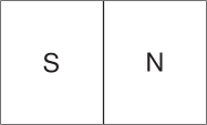
Figure 1: S/N bilayer.

Study of the proximity effect goes back to the beginning of the 1960’s and was reviewed in many publications (see, e.g. de Gennes (1964) and Deutscher and de Gennes (1969)). It was found that the critical temperature of the superconductor in a $S/N$ system decreased with increasing $N$ layer thickness. This behavior can be interpreted as the breaking down of some Cooper pairs due to the penetration of one of the electrons of the pairs into the normal metal where they are no longer attracted by the other electrons of the pairs.

At the same time, penetrating into the normal metal the Cooper pairs induce superconducting correlations. For example, the influence of the superconductivity on the physical properties of the $N$ metal manifests itself in the suppression of the density of states. Experiments determining the density of states of S/N bilayers with the help of tunneling spectroscopy were performed many years ago Toplicar and Finnemore (1977); Adkins and Kington (1969). While spatially resolved density of states were later measured by Gupta et al. (2004); Guéron et al. (1996); Anthore et al. (2003) (see FIG. 2).

Figure 2: Tunnelling density of states measured at 60 mK at the Au surface of different Nb/Au bilayers samples with varying Au thickness $d_{N}$. Adapted from Gupta, Cr tinon, Moussy, Pannetier, and Courtois (2004).

The simplest way to describe the proximity effect is to use the Ginzburg-Landau (G-L) equation for the order parameter $\Delta$ Ginzburg and Landau (1950). This equation is valid if the temperature is close to the critical temperature of the superconducting transition $T_{c}$. In this case all quantities can be expanded in the small parameter $\Delta/T_{c}$ and slow variations of the order parameter $\Delta$ in space.

Using the G-L equation written as

$$\xi_{GL}\frac{\partial^{2}\Delta\left(\mathbf{r}\right)}{\partial\mathbf{r}^{2}}+\Delta\left(\mathbf{r}\right)(\mbox{${\rm sgn}$}(T_{c,N,S}-T)-\Delta^{2}\left(\mathbf{r}\right)/\Delta_{0}^{2})=0\;.$$ (1)

one can describe the spatial distribution of the order parameter in any $N/S$ structure. Here $\xi_{GL}$ is the coherence length in the $N$ and $S$ regions at temperatures close to the critical temperatures $T_{cN,S}$. In the diffusive limit this length is equal to

$$\xi_{GL}=\sqrt{\pi D_{N,S}/8|T-T_{cN,S}|}$$ (2)

where $D_{N,S}$ is the diffusion coefficient in the $N$ and $S$ regions. The quantity $\Delta_{0}$ is the bulk value of the order parameter in the superconductor $S$. It vanishes when T reaches the transition temperature $T_{c}$.

It should be noticed though, that the region of the applicability of Eq. (1) for the description of the $S/N$ contacts is rather restricted. Of course, the temperature must be close to the transition temperature $T_{c}$ but this is not sufficient. The G-L equation describes variations of the order parameters correctly only if they are slow on the scales $v_{F}/T_{c}$ for the clean case or $\sqrt{D_{N,S}/T_{c}}$ in the diffusive “dirty” case. This can be achieved if the normal metal is a superconducting material taken at a temperature exceeding its transition temperature $T_{cN}$ and the transition temperatures $T_{cS}$ and $T_{cN}$ are close to each other. If this condition is not satisfied (e.g. $T_{cN}=0$) one should use more complicated equations even at temperatures close to $T_{cS}$, as we show below.

It follows from Eq. (1) that in the $S$ region, far from the $N/S$ interface, the order parameter $\Delta\left(\mathbf{r}\right)$ equals the bulk value $\Delta_{0}$, whereas in the $N$ region $\Delta\left(\mathbf{r}\right)$ decays exponentially to zero on the length $\xi_{N}$.

The order parameter $\Delta\left(\mathbf{r}\right)$ is related to the condensate function (or Gor’kov function)

$$f(t,t^{\prime})=<\psi_{\uparrow}(t)\psi_{\downarrow}(t^{\prime})>$$ (3)

via the self-consistency equation

$$\Delta_{N,S}(t)=\lambda_{N,S}f(t,t)\;,$$ (4)

where $\lambda_{N,S}$ is the electron-electron coupling constant leading to the formation of the superconducting condensate.

Eq.(1) describes actually a contact between two superconductors with different critical temperatures $T_{cN,S}$, when the temperature is chosen between $T_{cS}$ and $T_{cN}$. In the case of a real normal metal the coupling constant $\lambda_{N}$ is equal to zero and therefore $\Delta_{N}=0$. However, this does not imply that the normal metal does not possess superconducting properties in this case. The point is that many important physical quantities are related not to the order parameter $\Delta$ but to the condensate function $f$, Eq. (3). For example, the non-dissipative condensate current $j_{S}$ is expressed in terms of the function $f$ but not of $\Delta$. If the contact between the $N$ and $S$ regions is good, the condensate penetrates the normal metal leading to a finite value of $j_{S}\neq 0$ in this region.

In the general case of an arbitrary $\lambda_{N}$ it is convenient to describe the penetration of the condensate (Cooper pairs) into the ${N}$ region in the diffusive limit by the Usadel equation Usadel (1970) which is valid for all temperatures and for distances exceeding the mean free path $l$. This equation determines the so called quasiclassical Green’s functions (see Appendix A) which can be conveniently used in problems involving length scales larger than the Fermi wave length $\lambda_{F}$ and energies much smaller than the Fermi energy. Alternatively, one could try to find an exact solution (the normal and anomalous electron Green’s functions) for the Gor’kov equations, but this is in most of the cases a difficult task.

In order to illustrate the convenience of using the quasiclassical method we calculate now the change of the tunnelling density of states (DOS) in the normal metal due to the proximity effect with the help of the Usadel equation. The DOS is a very important quantity that can be measured experimentally and, at the same time, can be calculated without difficulties.

We consider the $S/N$ structure shown in FIG. 1 and assume that the system is diffusive (i.e. the condition $\epsilon\tau<<1$ is assumed to be fulfilled, where $\tau$ is the momentum relaxation time and $\epsilon$ is the energy) and that the transparency of the $S/N$ is low enough. In this case the condensate Green’s function $f(\epsilon)=\int dtf(t-t^{\prime})\exp(i\epsilon(t-t^{\prime}))$ is small in the $N$ region and the Usadel equation can be linearized (see Appendix A).

Assuming that the boundary between the superconductor and normal metal is flat and choosing the coordinate $x$ perpendicular to the boundary we reduce the Usadel equation in the $N$ region to the form

$$D_{N}\partial^{2}f/\partial x^{2}+2i\epsilon f=0\;,$$ (5)

where $D_{N}=v_{F}l/3$ is the classical diffusion coefficient.

The solution of this equation can be found easily and we write it as

$$f=f_{0}\exp\left(-x\sqrt{-2i\epsilon/D_{N}}\right)\;,$$ (6)

where $f_{0}$ is a constant that is to be found from the boundary conditions.

We see that the solution for the condensate function $f$ decays in the $N$ region exponentially at distances inversely proportional to $\sqrt{\epsilon}$. In many cases the main contribution to physical quantities comes from the energies $\epsilon$ of the order of the temperature, $\epsilon\sim T$. This means that the superconducting condensate penetrates the $N$ region over distances of the order of $\xi_{N}=\sqrt{D_{N}/2\pi T}$. At low temperatures this distance becomes very large, and if the thickness of the normal metal layer is smaller than the inelastic relaxation length, the condensate spreads throughout the entire $N$ region.

In order to calculate the DOS it is necessary to know the normal Green’s function $g$ which is related to the condensate function $f$ via the normalization condition (see Appendix A)

$$g^{2}-f^{2}=1$$ (7)

Eqs. (5) and (7) are written for the retarded Green’s function ($f=f^{R}$, see Appendix A). They are also valid for the advanced Green’s functions provided $(\epsilon+i0)$ is replaced by $(\epsilon-i0)$. The normalized density-of-states (we normalize the DOS to the DOS of non-interacting electrons) $\nu(\epsilon)$ is given by the expression

$$\nu(\epsilon)=\mathrm{Re}g(\epsilon)$$ (8)

As the condensate function $f$ is small, a correction $\delta\nu$ to the DOS due to the proximity effect is also small. In the main approximation the DOS $\nu$ is very close to its value in the absence of the superconductor, $\nu\approx 1$. Corrections to the DOS $\delta\nu$ are determined by the condensate function $f$. From Eq. (7) one gets

$$\delta\nu\approx f^{2}/2\;.$$

Now we consider another case when the function $f$ is not small and the correction $\delta\nu$ is of the order of unity. Then the linearized Eq. (5) may no longer be used and we should write a more general one. For a S/N system the general equation can be written as (see Appendix A)

$$-iD_{S,N}\partial(\hat{g}\partial\hat{g}/\partial x)_{S,N}/\partial x+\epsilon[\hat{\tau}_{3},\hat{g}_{S,N}]+[\hat{\Delta}_{S},\hat{g}_{S,N}]=0\;.$$ (9)

This non-linear equation contains the quasiclassical matrix Green’s function $\hat{g}$. Both normal $g$ and anomalous Green’s functions $f$ enter as elements of this matrix through the following relation (the phase in the superconductor is set to zero)

$$\hat{g}_{N}=g_{N}\hat{\tau}_{3}+f_{N}i\hat{\tau}_{2}\;,$$ (10)

where $\tau_{i}$, $i=1,2,3$ are Pauli matrices and $\left[A,B\right]=AB-BA$ is the commutator for any matrices $A$ and $B$.

We consider a flat $S/N$ interface normal to the $x$-axis. The normal metal occupies the region $0<x<d_{N}.$ We assume that in the normal metal $N$ there is no electron-electron interaction ($\lambda_{N}=0$, see Eq.(4)) so that in this region the superconducting order parameter vanishes, $\Delta_{N}=0.$ In the superconductor the matrix $\hat{\Delta}_{S}$ has the structure $\hat{\Delta}_{S}=\Delta i\hat{\tau}_{2}.$

At large distances from the $S/N$ interface the Green’s functions $\hat{g}_{S}$ of the superconductor do not depend on coordinates and the first term in Eq. (9) can be neglected. Then we obtain a simpler equation

$$\epsilon[\hat{\tau}_{3},\hat{g}_{S}]+\Delta[i\hat{\tau}_{2},\hat{g}_{S}]=0\;.$$ (11)

The solution for this equation satisfying the normalization condition (7) is

$$g_{BCS}=\epsilon/\xi_{\epsilon};\text{ }f_{BCS}=\Delta/\xi_{\epsilon}\;,$$ (12)

where $\xi_{\epsilon}=\sqrt{\epsilon^{2}-\Delta^{2}}$. Eq. (12) is just the BCS solution for a bulk superconductor.

In order to find the matrix $\hat{g}(x)$ both in the $S$ and $N$ regions, Eq.(9) should be complemented by boundary conditions and this is a non-trivial problem. Starting from the initial Hamiltonian $\hat{H}_{tot}$, Eq. (22), one does not need boundary conditions at the interface between the superconductor and the ferromagnet because the interface can be described by introducing a proper potential in the Hamiltonian. In this case the self-consistent Gor’kov equations can be derived.

However, deriving the Usadel equation, Eq. (178), we have simplified the initial Gor’kov equations using the quasiclassical approximation. Possible spatial variation of the interface potential on a very small scale, due to the roughness of the interface cannot be included in the quasiclassical equations. Nevertheless, this problem is avoided deriving the quasiclassical equations at distances from the interface exceeding the wavelength. In the diffusive case one should go away from the interface to distances larger than the mean free path $l$. In order to match the solutions in the superconducting and non-superconducting regions one should solve exact the equations near the interface and compare the asymptotic behavior of this solution at large distances with the solutions of the Usadel equation. This procedure is equivalent to solving the quasiclassical equations with some boundary conditions. These conditions were derived by Zaitsev (1984) and Kuprianov and Lukichev (1988) (see also Appendix A, where these conditions are discussed in more details). For the present case they can be written as

$$2\gamma_{S,N}(\hat{g}\partial\hat{g}/\partial x)_{S,N}=[\hat{g}_{S},\hat{g}_{N}]|_{x=0}$$ (13)

where $\gamma_{S,N}=R_{b}\sigma_{S,N}$, $R_{b},$ measured in units $\Omega cm^{2}$, is the $S/N$ interface resistance per unit area in the normal state, and $\sigma_{S,N}$ are the conductivities of the $S$ and $N$ metals in the normal state.

We assume that the thickness of the normal metal $d_{N}$ is smaller than the characteristic penetration length $\xi_{N}(\epsilon)=\sqrt{D_{N}/\epsilon}$ for a given energy $\epsilon$, that is $\epsilon<<D_{N}/d_{N}^{2}=E_{T}$. Then the functions $g$ and $f$ remain almost constant over the thickness of the metal, and for finding them, one can average the Usadel equation over the thickness. In other words, we assume that the thickness $d_{N}$ of the N layer satisfies the inequality

$$\;d_{N\text{ }}<<\sqrt{D_{N}/\epsilon},\text{ }\epsilon\sim\epsilon_{bN}$$ (14)

($\epsilon_{bN}$ is a characteristic energy in the DOS of the $N$ layer) and average Eq. (9) over the thickness $d_{N}$ considering $\hat{g}_{N}$ as a constant in the second term of this equation. Using the boundary condition, Eq.(13), the first term in Eq. (9) can be replaced after the integration by the commutator $[\hat{g}_{S},\hat{g}_{N}]|_{x=0}$. At $x=d_{N}$ the product $(\hat{g}\partial\hat{g}/\partial x)_{N}$ is zero because the barrier resistance $R_{b}(d_{N})$ is infinite (the current cannot flow into the vacuum). Finally, we obtain Zaitsev (1990)

$$(\epsilon+i\epsilon_{b}g_{S}(0))[\hat{\tau}_{3},\hat{g}_{N}]+\epsilon_{bN}if_{S}(0)[i\hat{\tau}_{2},\hat{g}_{N}]=0\;.$$ (15)

where $\epsilon_{bN}=(D_{N}/2\gamma_{N}d_{N})$ is a new characteristic energy that is determined by the $S/N$ interface resistance $R_{b}$. This equation looks similar to Eq.(11) after making the replacement $\hat{g}_{S}\rightarrow\hat{g}_{N}.$ The solution is similar to the solution (12)

$$g_{N}=\tilde{\epsilon}/\tilde{\xi}_{\epsilon};\text{ }f_{N}=\tilde{\epsilon}_{bN}/\tilde{\xi}_{\epsilon}\;,$$ (16)

where $\tilde{\epsilon}=\epsilon+i\epsilon_{bN}g_{S}(0),$ $\tilde{\xi}_{\epsilon}=\sqrt{\tilde{\epsilon}^{2}-\tilde{\epsilon}_{bN}^{2}},$ $\tilde{\epsilon}_{bN}=\epsilon_{bN}if_{S}(0).$ Therefore the Green’s functions in the $N$ layer $g_{N}$ and $f_{N}$ are determined by the Green’s functions on the $S$ side of the $S/N$ interface $g_{S}(0)$ and $f_{S}(0).$ In order to find the values of $g_{S}(0)$ and $f_{S}(0),$ one has to solve Eq. (9) on the superconducting side ($x<0$). However, provided the inequality

$$\gamma_{N}/\gamma_{S}=\sigma_{N}/\sigma_{S}<<1$$ (17)

is fulfilled one can easily show that, in the main approximation, the solution in the $S$ region coincides with the solution for bulk superconductors (12). If the transparency of the $S/N$ interface is not high, $\epsilon_{bN}<<\Delta$, the characteristic energies $\epsilon\sim\epsilon_{bN}$ are much smaller than $\Delta$ and the functions $g_{S}(0)$ and $f_{S}(0)$ are equal to: $g_{S}(0)\approx g_{BCS}(0)\approx\epsilon/i\Delta,$ $f_{S}(0)\approx f_{BCS}(0)\approx 1/i.$ For these energies the functions $g_{N}$ and $f_{N}$ have the same form as the BCS functions $g_{BCS}$ and $f_{BCS}$ (12) with the replacement $\Delta\rightarrow\epsilon_{bN}$

$$g_{N}=\frac{\epsilon}{\sqrt{\epsilon^{2}-\epsilon_{bN}^{2}}},\text{ \ }f_{N}=\frac{\epsilon_{bN}}{\sqrt{\epsilon^{2}-\epsilon_{bN}^{2}}}\;,$$ (18)

where $\epsilon_{bN}=D_{N}/(2R_{b}\sigma_{N}d_{N})$. The energy $\epsilon_{bN}$ can be represented in another form

$$\epsilon_{bN}=\frac{\pi^{2}}{2}(\frac{R_{Q}}{R_{b}k_{F}^{2}})\hbar\frac{v_{F}}{d_{N}}=\hbar\frac{v_{F}}{d_{N}}(\frac{T_{b}}{4})\;.$$ (19)

$R_{Q}=\hbar/e^{2}$ is the resistance quantum, $v_{F}$ and $k_{F}$ are the Fermi velocity and wave vector. When obtaining the latter expression, we used a relation between the barrier resistance $R_{b}$ and an effective coefficient of transmission $T_{b}$ through the S/N interface Kuprianov and Lukichev (1988); Zaitsev (1984): $R_{b}\sigma_{n}=(2/3)(l/T_{b}),$ where $l=v_{F}\tau$ is the mean free path, $T_{b}=<T(\theta)\cos\theta/(1-T(\theta)>,$ $\theta$ is the angle between the momentum of an incoming electron and the vector normal to the S/N interface, and $T(\theta)$ is the angle dependent transmission coefficient. The angle brackets mean an averaging over $\theta$.

An important result follows from Eq.(18): the DOS is zero at $|\epsilon|<\epsilon_{bN}$, i.e., $\epsilon_{bN}$ is a minigap in the excitation spectrum McMillan (1968). Remarkably, in the considered limit $\epsilon_{bN}<<\Delta$ the value of $\epsilon_{bN}$ does not depend on $\Delta$, but is determined by the interface transparency or, in other words, by the interface resistance $R_{b}$. The appearance of the minigap is related to Andreev reflections Andreev (1964).

Eq. (19) for the minigap is valid if the inequalities (14)   and $\epsilon_{bN}<\Delta$ are fulfilled. Both inequalities can be written as

$$(D_{N}/\Delta)/d_{b}<d_{N}<d_{b}$$ (20)

where $d_{b}=2R_{b}\sigma_{N}$ is a characteristic length. In the case of a small interface resistance $R_{b}$ or a large thickness of the N layer, that is, if the condition $\sqrt{\mathit{D}_{N}\mathit{/\Delta}},d_{b\text{ }}<d_{N}$ is fulfilled, the value of the minigap in the N layer is given by Golubov and Kupriyanov (1996)

$$\mathit{\epsilon}_{bN}\mathit{=c}_{1}\frac{D_{N}}{d_{N}^{2}}\mathit{\;}$$ (21)

where $c_{1}$ is a factor of the order 1. This result has been obtained from a numerical solution of the Usadel equation. The DOS for the case of arbitrary thickness $d_{N}$  and interface transparency was calculated by Pilgram et al. (2000).

The situation changes in the clean limit. Let us consider, for example, a normal slab of a thickness $d_{N}$ in contact with an infinite superconductor. If the Thouless energy $E_{Th}=v_{F}/d_{N}$ is less than $\Delta$, then discrete energy levels $\epsilon_{n}$ appear Saint-James (1964) in the N region due to Andreev reflections Andreev (1964). As a result, the DOS has sharp peaks at $\epsilon=\epsilon_{n}$  (for a recent review see Deutscher (2005)). If $E_{Th}$ is much larger than $\Delta,$ the DOS $\nu(\epsilon)$ is zero at $\epsilon=0$ and increases with increasing the energy $\epsilon$ (no gap). However, this is true only for such a simple geometry. For samples of more complicated shapes the behavior of the DOS $\nu(\epsilon)$ depends on whether the electron dynamics in the N region is chaotic or integrable Melsen et al. (1996); Lodder and Yu.V.Nazarov (1998); Pilgram et al. (2000); Taras-Semchuk and Altland (2001); Beenakker (1997).

Finally, it has been shown by Altland et al. (2000) and Ostrovsky et al. (2001) that mesoscopic fluctuations smear out the singularity in the DOS at $|\epsilon|=\epsilon_{bN}$ and the DOS in the diffusive limit is finite, although small, for $|\epsilon|<\epsilon_{bN}.$ The minigap discussed above has been observed on a Nb/Si bilayer system and on a Pb/Ag granular system by Heslinga et al. (1994); Kouh and Valles (2003), respectively.

From this analysis we see that the proximity effect changes the DOS of the normal metal which acquires superconducting properties. In the next section we will focus our attention on the case that the normal metal is a ferromagnet. We will see that new interesting physics will arise from the mutual interaction of superconductivity and magnetism.

II.2 Superconductor-ferromagnet structures with an uniform magnetization

In this section we consider the proximity effect between a superconductor $S$ and a ferromagnet $F$. We assume that the ferromagnet is a metal and has a conduction band. In addition, there is an exchange field due to spins of electrons of other bands.

As has been already mentioned, the effective exchange field acts on spins of the conduction electrons in the ferromagnet, and an additional term $\hat{H}_{ex}$ describing this action appears in the total Hamiltonian (for more details see Appendix A)

$$\hat{H}_{tot}=\hat{H}+\hat{H}_{ex}$$ (22)

$$\hat{H}_{ex}=-\int d^{3}\mathbf{r}\psi_{\alpha}^{+}\left(\mathbf{r}\right)\left(\mathbf{h}\left(\mathbf{r}\right)\sigma_{\alpha\beta}\right)\psi\left(\mathbf{r}\right)d\mathbf{r}$$ (23)

where $\psi^{+}\left(\psi\right)$ are creation and destruction operators, $\mathbf{h}$ is the exchange field, $\mathbf{\sigma}_{\alpha\beta}$ are Pauli matrices, and $\alpha,\beta$ are spin indices. The Hamiltonian $\hat{H}$ stands for a non-magnetic part of the Hamiltonian. It includes the kinetic energy, impurities, external potentials, etc. and is sufficient to describe all properties of the system in the absence of the exchange field.

The energy of the spin-up electrons differs from the energy of the spin-down electrons by the Zeeman energy $2h$. Due to the presence of the term $\hat{H}_{ex}$ describing the exchange interaction all functions, including the condensate Green’s function $f$, are generally speaking non-trivial matrices in the spin space with non-zero diagonal and off-diagonal elements.

The situation is simpler if the direction of the exchange field does not depend on coordinates. In this case, choosing the $z$-axis along the direction of $\mathbf{h}$ one can consider electrons with spin “up” and “down” separately. In this Section we concentrate on this case. This can help the reader to understand several interesting effects and get an intuition about what one can expect from the presence of the exchange field. The results of this section will also help in understanding which effects in the superconductor-ferromagnet structures can be considered as rather usual and what kind of behavior is “exotic”. We will see that the exotic phenomena occur in cases when the exchange field is not homogeneous and therefore postpone their discussion until the next chapters.

If the exchange field $h$ is homogeneous the matrix $\hat{f}$ describing the condensate $\hat{f}$ is diagonal and can be represented in the form

$$\hat{f}=f_{3}\hat{\sigma}_{3}+f_{0}\hat{\sigma}_{0}\;$$ (24)

where $f_{3}$ is the amplitude of the singlet component and $f_{0}$ is the amplitude of the triplet component with zero projection of the magnetic moment of Cooper pairs on the $z$ axis ($S_{z}=0$). Note that in the case of a ${S/N}$ structure the condensate function has a singlet structure only, i.e. it is proportional to $\hat{\sigma}_{3}$. The presence of the exchange field leads to the appearance of the triplet term proportional to $\hat{\sigma}_{0}$

The amplitudes of the singlet and triplet components are related to the correlation functions $\left\langle\psi_{\alpha}\psi_{\beta}\right\rangle$ as follows Legget (1975); Vollhardt and Wölfle (1990)

$$f_{3}(t) \sim \left\langle\psi_{\uparrow}(t)\psi_{\downarrow}(0)\right\rangle-\left\langle\psi_{\downarrow}(t)\psi_{\uparrow}(0)\right\rangle\;,$$

$$f_{0}(t) \sim \left\langle\psi_{\uparrow}(t)\psi_{\downarrow}(0)\right\rangle+\left\langle\psi_{\downarrow}(t)\psi_{\uparrow}(0)\right\rangle\;,$$ (25)

One can see that a permutation of spins does not change the function $f_{3}(0),$ whereas such a permutation leads to a change of the sign of $f_{0}\left(0\right)$. This means that the amplitude of the triplet component taken at equal times is zero in agreement with the Pauli exclusion principle. Later we will see that in the case of a non-homogeneous magnetization all triplet components including $\left\langle\psi_{\uparrow}(t)\psi_{\uparrow}(0)\right\rangle$ and $\left\langle\psi_{\downarrow}(t)\psi_{\downarrow}(0)\right\rangle$ differ from zero.

Once one determines the condensate function, Eq. (24), one is able to determine physical quantities ,as DOS, the critical temperature $T_{C}$, or the Josephson critical current through a S/F/S junction.

Next paragraphs are devoted to a discussion of these physical properties in $F/S$ systems with homogeneous magnetization.

II.2.1 Density of states (DOS)

In this section we discuss the difference between the DOS in ${S/N}$ and ${S/F}$ structures. General equations for the quasiclassical Green’s functions describing the system can be written but they are rather complicated (see Appendix A). In order to simplify the problem and, at the same time, give the basic idea about the effects it is sufficient to consider some limiting cases. This will be done in the present section leaving the general equations for the Appendix A.

In the case of a weak proximity effect, the condensate function $\hat{f}$ is small outside the $S$ region. We consider again the diffusive limit. Then, the general Eq. (178) can be linearized and one obtains an equation for the matrix $\hat{f}$   similar to Eq.(5) but containing an extra term due to the exchange field $h$

$$D_{F}\partial^{2}\hat{f}_{F}/\partial x^{2}+2i(\epsilon\hat{\sigma}_{0}+h\hat{\sigma}_{3})\hat{f}_{F}=0\;.$$ (26)

The subscript $F$ stands for the $F$ region.

In the absence of the exchange field $h$, Eq. (26) reduces to Eq. (5). It is important to emphasize that Eq. (26) is valid for a homogeneous $h$ only. Any variation of $h$ in space makes the equation much more complicated.

Eq. (26) should be complemented by boundary conditions which take the form (see Appendix A)

$$\gamma_{F}\partial\hat{f}_{F}/\partial x=-\hat{f}_{S}$$ (27)

where $\gamma_{F}=R_{b}\sigma_{F}$, $R_{b}$ is the boundary resistance per unit area, $\sigma_{F}$ is the conductivity of the $F$ region, $\hat{f}_{F,S}$ are the condensate matrix functions in the $F$ and $S$ regions. Since we assume a weak proximity effect, a deviation of the $\hat{f}_{S}$ from its $BCS$ value $\hat{f}_{BCS}=\hat{\sigma}_{3}f_{BCS}$ is small. Therefore on the right-hand side of Eq.(27) one can write $\hat{f}_{S}\approx\hat{\sigma}_{3}f_{BCS},$ where $f_{BCS}$ is defined in Eq.(9). At the ferromagnet/vacuum interface the boundary condition is given by the usual expression $\partial_{x}\hat{f}_{F}=0$, which follows from the condition $R_{b}\rightarrow\infty$.

Using Eq. (27), one can easily solve Eq. (26). We assume, as in the previous section, that the normal metal (ferromagnet) is in a contact with the superconductor at $x=0$ ($x$ is the coordinate perpendicular to the interface). The other boundary of the ferromagnet is located at $x=d_{F}$ and the space at $x>d_{F}$ is empty.

The proper solution for the diagonal matrix elements $f_{\pm}\equiv f_{11(22)}$ can be written as

$$f_{\pm}(x)=\left\{\begin{array}[]{cc}\pm\frac{f_{BCS}}{\kappa_{\epsilon\pm}\gamma_{F}}\frac{\cosh(\kappa_{\epsilon\pm}(x-d_{F}))}{\sinh(\kappa_{\epsilon\pm}d_{F})}&0<x<d_{F}\\ \text{\ }0\text{ }&x>d_{F}\end{array}\right.\text{ }\;.$$ (28)

Here $\kappa_{\epsilon\pm}=\sqrt{-2i(\epsilon\pm h)/D_{F}}$ is a characteristic wave vector that determines the inverse penetration depth of the condensate functions $f_{0,3}$ into the ferromagnet.

Usually, the exchange energy $h$ is much larger than the energy $\epsilon$ ($\epsilon\propto\max\{\Delta,T\}$). This means that the condensate penetration depth $\xi_{F}=\sqrt{D_{F}/h}$ is much shorter than the penetration depth into a normal (non-magnetic) metal $\xi_{N}$. The strong suppression of the condensate in the ferromagnet is caused by the exchange interaction that tries to align the spins of  electrons parallel to the magnetization. This effect destroys the Cooper pairs with zero total magnetic moment.

It is worth mentioning that the condensate function $f_{\pm}$ experiences oscillations in space. Indeed, for a thick $F$ layer  ($d_{F}>>\xi_{F}$)  we obtain from Eq. (28).

$$f_{\pm}=\pm\frac{\Delta}{E_{\epsilon}\kappa_{F\pm}\gamma_{F}}\exp(-x/\xi_{F})[\cos(x/\xi_{F})\pm i\sin(x/\xi_{F})].$$ (29)

where $E_{\epsilon}=\sqrt{\epsilon^{2}-\Delta^{2}},\kappa_{F\pm}=\kappa_{\epsilon\pm}(\epsilon)$ at $\epsilon=0$. The damped oscillations of $\;f_{\pm}$ lead to many interesting effects and, in particular, to a non-monotonic dependence of the critical temperature on the thickness $d_{F}$ of a $F/S$ bilayer which will be discussed in the next section.

In order to calculate the DOS we have to use the normalization condition, Eq. (7), which is also valid for the matrix elements $f_{\pm}$ and $g_{\pm}$. Thus, for $g_{\pm}$ we obtain $g_{\pm}=\sqrt{1+f_{\pm}^{2}}$, which can be written for small $f_{\pm}$ as $g_{\pm}\approx 1+f_{\pm}^{2}/2$. Then the correction to the normalized DOS in the $F$ region $\delta\nu_{F}=\nu_{F}-1$ takes the form

$$\delta\nu_{F}(x)=\mathrm{Re}(f_{+}^{2}+f_{-}^{2})/4\;.$$ (30)

Substituting Eq. (28) into Eq.(30), we obtain finally the DOS variation at the edge of the F film

$$\delta\nu_{F}(d_{F}) = (1/4)\mathrm{Re}\left\{(\frac{f_{BCS}}{\gamma_{F}})^{2}\left[(\kappa_{\epsilon+}\sinh(\kappa_{\epsilon+}d_{F}))^{-2}+\right.\right.$$ (31)

$$\left.\left.+(\kappa_{\epsilon-}\sinh(\kappa_{\epsilon-}d_{F}))^{-2}\right]\right\}\;.$$

In FIG. 3 we plot the function $\delta\nu_{F}(\epsilon)$ for different thicknesses $d_{F}$ and $h/\Delta=20$. It is seen that at zero energy $\epsilon=0$ the correction to DOS $\delta\nu_{F}$ is positive for $F$ films with $d_{F}=0.8\xi_{0}$ while it is negative for films with $d_{F}=0.5\xi_{0}$ where $\xi_{0}=\sqrt{D_{F}/\Delta}$.

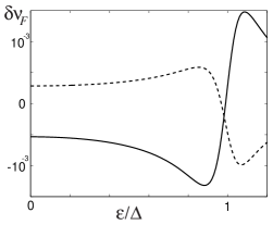
Figure 3: Calculated change of the local density of states for a S/F bilayer at the outer F interface. The solid line corresponds to a F thickness $d_{F}=0.5\xi_{0}$, where $\xi_{0}=\sqrt{D_{F}/\Delta}$, while the dashed one corresponds to $d_{F}=0.8\xi_{0}$. The latter curve is multiplied by a factor of 10.

Such a behavior of the DOS, which is typical for S/F systems, has been observed experimentally by Kontos et al. (2001) in a bilayer consisting of a thin PdNi film ($5nm<d_{F}<7.5nm$) on the top of a thick superconductor. The DOS was determined by tunnelling spectroscopy. This type of dependence of $\delta\nu_{N}$ on $d_{N}$ can also be obtained in $N/S$ contacts but for finite energies $\epsilon$. In the $F/S$ contacts the energy $\epsilon$ is shifted, $\epsilon\rightarrow\epsilon\pm h$ (time-reversal symmetry breaking) and this leads to a non-monotonic dependence of $\nu_{F}$ on the thickness $d_{F}$ even at zero energy. On the other hand, a non oscillatory behavior of the DOS $\nu(\epsilon)$ has been found recently in experiments on Nb/CoFe bilayers Reymond et al. (2000). The discrepancy between the existing theory and the experimental data may be due to the small thicknesses of the ferromagnetic layer ($0.5nm<d_{F}<2.5nm$) which is comparable with the Fermi wave length $\lambda_{F}\approx 0.3nm$. Strictly speaking, in this case the Usadel equation cannot be applied.

The DOS in $F/S$ structures was studied theoretically in many papers. Halterman and Valls (2002b) studied the DOS variation numerically for ballistic $F/S$ structures. The DOS in quasiballistic $F/S$ structures was investigated by Baladie and Buzdin (2001), Bergeret et al. (2002b) and Zareyan et al. (2001) and for dirty $F/S$ structures by Fazio and Lucheroni (1999) and Buzdin (2000). The subgap in a dirty S/F/N structure was investigated in a recent publication by Golubov et al. (2005).

It is interesting to note that in the ballistic case ($\tau h>>1$, $\tau$ is the momentum relaxation time) the DOS in the $F$ layer is constant in the main approximation in the parameter $1/(\tau h)$ while in the diffusive case ($\tau h<<1$) it experiences the damped oscillations. The reason for the constant DOS in the ballistic case is that both the parts of $f$ , the symmetric and antisymmetric in the momentum space, contribute to the DOS. Each of them oscillates in space. However, while in the diffusive case the antisymmetric part is small, in the ballistic case the contributions of both parts to the DOS are equal to each other, but opposite in sign, thus compensating each other.

Finally, we would like to emphasize that both, the singlet and triplet components, contribute to the DOS. As it is seen from Eq.(30), the changes of the DOS can be represented in the form $\delta\nu_{F}={\rm Re}(f_{0}^{2}+f_{3}^{2})/4$, which demonstrates explicitly this fact.

II.2.2 Transition temperature

As we have seen previously, the exchange field affects greatly the singlet pairing in conventional superconductors. Therefore the critical temperature of the superconducting transition $T_{c}$ is considerably reduced in $S/F$ structures with a high interface transparency.

The critical temperature for $S/F$ bilayer and multilayered structures was calculated in many works Radovic et al. (1991); Demler et al. (1997); Khusainov and Proshin (1997); Tagirov (1998); Baladie and Buzdin (2003); Fominov et al. (2002); Bagrets et al. (2003); Fominov et al. (2003); Proshin and Khusainov (1998, 1999); Proshin et al. (2001); Buzdin and Kupriyanov (1991); Tollis et al. (2005); You et al. (2004); Baladie et al. (2001). Experimental studies of the $T_{c}$ were also reported in many publications Jiang et al. (1995); Mühge et al. (1998); Aarts et al. (1997); Lazar et al. (2000); Gu et al. (2002a). A good agreement between theory and experiment has been achieved in some cases (see FIG. 4).

Figure 4: Dependence of the superconducting transition temperature on the thickness of the Fe layer as determined by resistivity measurements. The dashed line is a fit assuming a perfect interface transparency while the solid line corresponds to a non-perfect interface. Adapted from Lazar, Westerholt, Zabel, Tagirov, Goryunov, Garif’yanov, and Garifullin (2000).

One has to mention that, despite of many papers published on this subject, the problem of the transition temperature $T_{c}$ in the $S/F$ structures is not completely clear. For example, Jiang et al. (1995) and Ogrin et al. (2000) claimed that the non-monotonic dependence of $T_{c}$ on the thickness of the ferromagnet observed on ${Gd/Nb}$ samples was due to the oscillatory behavior of the condensate function in ${F}$. However, Aarts et al. (1997) in an other experiment on ${V/FeV}$ have shown that the interface transparency plays a crucial role in the interpretation of the experimental data that showed both non-monotonic and monotonic dependence of $T_{c}$ on $(d_{F})$. In other experiments Bourgeois and Dynes (2002) the critical temperature of the bilayer Pb/Ni decreases with increasing $d_{F}$ in a monotonic way.

From the theoretical point of view the $T_{c}$ problem in a general case cannot be solved exactly. In most papers it is assumed that the transition to the superconducting state is of second order, i.e. the order parameter $\Delta$ varies continuously from zero to a finite value with decreasing the temperature $T$. However, generally this is not so.

Let us consider, for example, a thin $S/F$ bilayer with thicknesses obeying the condition: $d_{F}<\xi_{F}$, $d_{S}<\xi_{S}$, where $d_{F,S}$ are the thicknesses of the $F(S)$ layer. In this case the Usadel equation can be averaged over the thickness (see for instance, Bergeret et al. (2001b)) and reduced to an equation describing an uniform magnetic superconductor with an effective exchange energy $\tilde{h}$ and order parameter $\tilde{\Delta}$.

This problem can easily be solved. The Green’s functions $g_{\pm}$ and $f_{\pm}$ are given by

$$g_{\pm}=\frac{\epsilon\pm\tilde{h}}{E_{\epsilon}},\text{ \ }f_{\pm}=\frac{\tilde{\Delta}}{E_{\epsilon}}\;,$$ (32)

where $E_{\epsilon}=\sqrt{(\epsilon\pm\tilde{h})^{2}-\tilde{\Delta}^{2}},$ $\tilde{h}=r_{F}h$, $\tilde{\Delta}=r_{S}\Delta$, $r_{F}=1-r_{S}=\nu_{F}d_{F}/(\nu_{F}d_{F}+\nu_{S}d_{S})$. In this case the Green’s functions are uniform in space and have the same form as in a magnetic superconductors or in a superconducting film in a parallel magnetic field acting on the spins of electrons.

The difference between the $S/F$ bilayer system and a magnetic superconductors is that the effective exchange energy $\tilde{h}$ depends on the thickness of the $F$ layer and may be significantly reduced in comparison with its value in a bulk ferromagnet. A thin superconducting film in a strong magnetic field $H=\tilde{h}/\mu_{B}$ ($\mu_{B}$ is an effective Bohr magneton) is described by the same Green’s functions. The behavior of these systems and, in particular, the critical temperature of the superconducting transition $T_{c}$, was studied long ago by Larkin and Ovchinikov (1964); Fulde and Ferrell (1965); Sarma (1963); Maki (1968). It was established that both first and second order phase transitions may occur in these systems if $\tilde{h}$ is less or of the order of $\tilde{\Delta}$. If the effective exchange field $\tilde{h}$ exceeds the value $\tilde{\Delta}/\sqrt{2}\approx 0.707\tilde{\Delta},$ the system remains in the normal state (the Clogston (1962) and Chandrasekhar (1962) limit). Independently from each other Larkin and Ovchinikov (1964) and Fulde and Ferrell (1965) found that in a clean system and in a narrow interval of $\tilde{h}$ the homogeneous state is unstable and an inhomogeneous state with the order parameter varying in space is established in the system. This state, denoted as the Fulde-Ferrel-Larkin-Ovchinnikov (LOFF) state. has not been observed yet in bulk superconductors. In bilayered $S/F$ systems such a state cannot be realized because of a short mean free path.

In the case of a first order phase transition from the superconducting to the normal state the order parameter $\Delta$ drops from a finite value to zero. The study of this transition requires the use of nonlinear equations for $\Delta$. It was shown by Tollis (2004) that under some assumptions both the first and second order phase transitions may occur in a S/F/S structure.

In the case of a second order phase transition one can linearize the corresponding equations (the Eilenberger or Usadel equation) for the order parameter and use the Ginzburg-Landau expression for the free energy assuming that the temperature $T$ is close to the critical temperature $T_{c}$. Just this case was considered in most papers on this topic. The critical temperature of an $S/F$ structure can be found from an equation which is obtained from the self-consistency condition Eq. (4). In the Matsubara representation it has the form

$$\ln\frac{T_{c}}{T_{c}^{\ast}}=(\pi T_{c}^{\ast})\sum_{\omega}(\frac{1}{|\omega_{n}|}-if_{\omega}/\Delta),$$ (33)

where $T_{c}$ is the critical temperature in the absence of the proximity effect and $T_{c}^{\ast}$ is the critical temperature with taking into account the proximity effect.

The function $f_{\omega}$ is the condensate (Gor’kov) function in the superconductor; it is related to the function $f_{S3}(\epsilon)$ as $f_{S3}(i\omega_{n})=f_{\omega},$ where $\omega_{n}=\pi(2n+1)$ is the Matsubara frequency. Strictly speaking, Eq.(33) is valid for a superconducting film with a thickness smaller than the coherence length $\xi_{S}$ because in this case $f_{\omega}$ is almost constant in space.

The quasiclassical Green’s function $f_{\omega}$ obeys the Usadel equation (in the diffusive case) or the more general Eilenberger equation. One of these equations has to be solved by using the boundary conditions at the $S/F$ interface (or $S/F$ interfaces in case of multilayered structures). This problem was solved in different situations in many works where an oscillation of $T_{c}$ as a function of the F thickness was predicted (see FIG. 4). In most of these papers it was assumed that magnetization vectors $\mathbf{M}$ in different $F$ layers are collinear. Only Fominov et al. (2003) considered the case of an arbitrary angle $\alpha$ between the $\mathbf{M}$ vectors in two $F$ layers separated by a superconducting layer.

As mentioned previously, in this case the triplet components with all projections of the spin $S$ of the Coopers pair arise in the $F/S/F$ structure. It was shown that $T_{c}$ depends on $\alpha$ decreasing from a maximum value $T_{c\max}$ at $\alpha=0$ to a minimum value $T_{c\min}$ at $\alpha=\pi.$ We will not discuss the problem of $T_{c}$ for $S/F$ structures in detail because this problem is discussed in other review articles Izyumov et al. (2002); Buzdin (2005a).

II.2.3 The Josephson effect in SFS junctions

The oscillations of the condensate function in the ferromagnet (see Eq.(29)) lead to interesting peculiarities not only in the dependence $T_{c}(d_{F})$ but also in the Josephson effect in the ${S/F/S}$ junctions. Although, as it has been mentioned in the previous section, the experimental results concerning the dependence $T_{c}(d_{F})$ are still controversial, there is a more clear evidence for these oscillations in experiments on the Josephson current measurements that we will discuss here.

It turns out that under certain conditions the Josephson critical current $I_{c}$ changes its sign and becomes negative. In this case the energy of the Josephson coupling $E_{J}=(\hbar I_{c}/e)[1-\cos\varphi]$ has a minimum in the ground state when the phase difference $\varphi$ is equal not to $0$, as in ordinary Josephson junctions, but to $\pi$ (the so called $\pi-$junction).

This effect was predicted for the first time by Bulaevskii et al. (1977). The authors considered a Josephson junction consisting of two superconductors separated by a region containing magnetic impurities. The Josephson current through a $S/F/S$ junction was calculated for the first time by Buzdin et al. (1982). Different aspects of the Josephson effect in S/F/S structures has been studied in many subsequent papers (Buzdin and Kupriyanov, 1991; Radovic et al., 2003; Fogelström, 2000; Barash et al., 2002; Golubov et al., 2002a; Heikkilä et al., 2000; Chtchelkatchev et al., 2001; Zyuzin et al., 2003, e.g). Recent experiments confirmed the $0$-$\pi$ transition of the critical current in S/F/S junctions Ryazanov et al. (2001); Kontos et al. (2002); Blum et al. (2002); Bauer et al. (2004); Sellier et al. (2004).

In the experiments of Ryazanov et al. (2001) and Blum et al. (2002), $Nb$ is used as a superconductor and a $Cu_{x}Ni_{1-x}$ alloy as a ferromagnet. Kontos et al. (2002) used a more complicated $S_{1}/F/I/S$ structure, where $S_{1}$ is a $Nb/Al$ bilayer, $S$ is $Nb$, $I$ is the insulating $Al_{2}O_{3}$ layer and $F$ is a thin ($40$Å$<d_{F}<150$Å) magnetic layer of a $PdNi$ alloy. All these structures exhibit oscillations of the critical current $I_{c}$.

Figure 5: Measurement of the critical current $I_{c}$ as a function of the temperature for a Nb/Cu_0.48Ni_0.52/Nb junction. The thickness of the CuNi layer is $d_{F}=22$nm. Adapted from Ryazanov, Oboznov, Rusanov, Veretennikov, Golubov, and Aarts (2001)

In FIG. 5 the temperature dependence of $I_{c}$ measured by Ryazanov et al. (2001) is shown. It is seen that the critical current in the junction with $d_{F}=27nm$ turns to zero at $T\approx 2$ $K$, rises again with increasing temperature and reaches a maximum at $T\approx 5.5$ $K$. If temperature increases further, $I_{c}$ decreases. In FIG. 6 we also show the dependence of $I_{c}$ on the thickness $d_{F}$ measured by Blum et al. (2002). The measured oscillatory dependence is well fitted with the theoretical dependence calculated by Buzdin et al. (1982) and Bergeret et al. (2001c).

Figure 6: Critical current of a Nb/Cu/Ni/Cu/Nb junction as a function of the Ni layer thickness $d$. The squares are the measured points. The theoretical fits are done according to Buzdin et al. (1982) (dashed line) and Bergeret et al. (2001c) (solid line). Adapted from Blum, A. Tsukernik, and Palevski (2002)

The $\pi$-state in a Josephson junction leads to some observable phenomena. As was shown by Bulaevskii et al. (1977), a spontaneous supercurrent may arise in a superconducting loop with a ferromagnetic $\pi$-junction. This current has been measured by Bauer et al. (2004). Note also that the fractional Shapiro steps in a ferromagnetic $\pi$-junction were observed by Sellier et al. (2004) at temperatures at which the critical current $I_{c}$ turns to zero.

Oscillations of the Josephson critical current $I_{c}$ are related to the oscillatory behavior of the condensate function $f$ in space (see Eq.(29)). The critical current $I_{c}$ in a $S/F/S$ junction can easily be obtained once the condensate function in the $F$ region is known. We use the following formula for the superconducting current $I_{S}$ in the diffusive limit which follows in the equilibrium case from a general expression (see Appendix A)

$$\;I_{S}=L_{y}L_{z}\sigma_{F}(i\pi T/4e)\sum_{\omega}Tr(\hat{\tau}_{3}[\;\check{f}_{+}\partial\;\check{f}_{+}/\partial x+\;\check{f}_{-}\partial\;\check{f}_{-}/\partial x]),$$ (34)

where $L_{y}L_{z}$ is the area of the interface and $\sigma_{F}$ is the conductivity of the $F$ layer.

In the considered case of a non-zero phase difference the condensate functions $f_{\pm}$ are matrices in the particle-hole space. If in Eq.(34) instead of $f_{\pm}$ we write a 4$\times$4 matrix for $\check{f}$, then $\Delta$ is given by $\hat{\Delta}=\Delta(i\hat{\tau}_{2}\cos(\varphi/2)\mp i\hat{\tau}_{1}\sin(\varphi/2))\hat{\sigma}_{3}.$ We set the phase of the right (left) superconductor equal to $\pm\varphi/2$. For simplicity we assume that the overlap between the condensate functions $f_{\pm}$ induced in the $F$ region by each superconductor is small. This assumption is correct in the case $d_{F}>>\xi_{F}$. Under this assumption the condensate function may be written in the form of two independently induced $f$ functions

$$\;\hat{f}_{\pm}(x) = (1/\xi_{\epsilon}\kappa_{F\pm}\gamma_{F})i\hat{\tau}_{2}[\hat{\Delta}_{l}\exp(-\kappa_{\epsilon\pm}(x+d_{F}/2)$$ (35)

$$+ \hat{\Delta}_{r}\exp(-\kappa_{\epsilon\pm}(-x+d_{F}/2)].$$

Here $\hat{\Delta}_{r(l)}$ is the order parameter in the right (left) superconductor. Substituting Eq.(35) into Eq.(34), we get

$$\;I_{S}\equiv I_{c}\sin(\varphi) = 4\pi T(L_{y}L_{z})\sigma_{F}/(\kappa_{F}\gamma_{F}^{2})\exp(-d_{F}/\xi_{F})$$ (36)

$$\cos(d_{F}/\xi_{F})\sum_{\omega}\frac{\Delta^{2}}{\Delta^{2}+\omega^{2}}\sin\varphi.$$

When deriving Eq.(36), it was assumed that the exchange energy $h$ is much larger than both $T$ and $\Delta.$

Calculating the sum in Eq. (36), we come to the final formula for the critical current

$$\;I_{c}=\Delta\tanh(\Delta/2T)\sigma_{F}/(\kappa_{F}\gamma_{F}^{2})\exp(-d_{F}/\xi_{F})\cos(d_{F}/\xi_{F}).$$ (37)

As expected, according to Eq.(37)  the critical current oscillates with varying the thickness of the ferromagnet $d_{F}$. The period of these oscillations gives the value of $\xi_{F}$ and therefore the value of the exchange energy $h.$ For example, according to the experiments on Nb/CuNi performed by Blum et al. (2002) $h\approx 110meV$, which is a quite reasonable value for CuNi.

The non-monotonic dependence of the critical current on temperature observed by Ryazanov et al. (2001) can be obtained only in the case of an exchange energy $h$ comparable with $\Delta$ (at least, the ratio $h/\Delta$ should not be too large). If the exchange energy were not too large, the effective penetration length $\xi_{F,eff}$ would be temperature dependent. According to estimates presented by Ryazanov et al. $h\approx 30K$, which means that the exchange energy in this experiment was much smaller than in the one performed by Blum et al. and by Kontos et al. (in the last reference $h\approx 35meV$).

The conditions under which the $\pi-$ state is realized in $S/F/S$ Josephson junctions of different types were studied theoretically in many papers Buzdin and Kupriyanov (1991); Buzdin and Vujicic (1992); Chtchelkatchev et al. (2001); Krivoruchko and Koshina (2001a); Li et al. (2002); Buzdin and Baladie (2003). In all these papers it was assumed that the ferromagnet consisted of a single domain with a magnetization $M$ fixed in space. The case of a $S/F/S$ Josephson junction with a two domain ferromagnet was analyzed by Blanter and Hekking (2004). The Josephson critical current $I_{c}$ was calculated for parallel and anti-parallel magnetization orientations in both ballistic and diffusive limits. It turns out that in such a junction the current $I_{c}$ is larger for the anti-parallel orientation.

A similar effect arises in a $S/F/S$ junction with a rotating in space magnetization, as it was shown by Bergeret et al. (2001c). In this case not only the singlet and triplet component with projection $S_{z}=0$, but also the triplet component with $S_{z}=\pm 1$ arises in the ferromagnet. The last component penetrates the ferromagnet over a large length of the order of $\xi_{N}$ and contributes to the Josephson current.

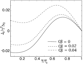
Figure 7: Dependence of the critical current on T for $h\tau=0.06$,$\Delta_{0}\tau=0.03$, $d/l=\pi$ and different values of $Ql$. Here $\tau$ is the momentum relaxation time.

In FIG. 7 the temperature dependence of the critical current is presented for different values of $Ql,$ where $Q=2\pi/L_{m}$, $L_{m}$ is the period of the spatial rotation of the magnetization and $l$ is the mean free path. It is seen that at $Q=0$ (homogeneous ferromagnet) and low temperatures $T$ the critical current $I_{c}$ is negative ($\pi-$ state$)$, whereas with increasing temperature, $I_{c}$ becomes positive ($0-$ state). If $Q$ increases, the interval of negative $I_{c}$ gets narrower and disappears completely at $Ql\approx 0.04$, that is, the $S/F/S$ structure with a non-homogeneous $M$ is an ordinary Josephson junction with a positive critical current.

It is interesting to note that the $\pi$-type Josephson coupling may also be realized in $S/N/S$ junctions provided the distribution function of quasiparticles $n(\epsilon)$ in the $N$ region deviates significantly from the equilibrium. This deviation may be achieved with the aid of a non-equilibrium quasiparticles injection through an additional electrode in a multiterminal $S/N/S$ junction. The Josephson current in such a junction is again determined by Eq.(34) in which one has to put $h=0,$ $f_{+}=f_{-}$ and replace $\tanh(\epsilon\beta)=(1-2n(\epsilon))$ by $(1/2)[\tanh((\epsilon+eV)\beta)+\tanh((\epsilon-eV)\beta)],$ where $V$ is a voltage difference between $N$ and $S$ electrodes.

At a certain value of $V$ the critical current changes sign. Thus, there is some analogy between the sign reversal effect in a ${S/F/S}$ junction and the one in a multiterminal ${S/N/S}$ junction under non-equilibrium conditions.

Indeed, when calculating $I_{S}$ in a multiterminal ${S/N/S}$ junction one can shift the energy by $eV$ or $-eV$. Then the function $(1/2)[\tanh((\epsilon+eV)\beta)+\tanh((\epsilon-eV)\beta)]$ is transformed into $\tanh(\epsilon\beta)$ while in the other functions one performs the substitution $\epsilon\rightarrow\epsilon\pm eV$. So, we see that $eV$ is analogous to the exchange energy $h$ that appears in the case of a ${S/F/S}$ junction.

The sign reversal effect in a multiterminal $S/N/S$ junction under non-equilibrium conditions has been observed by Baselmans et al. (1999) and studied theoretically by Volkov (1995); Yip (1998); Wilhelm et al. (1998). Later Heikkilä et al. (2000) studied theoretically a combined effect of a non-equilibrium quasiparticle distribution on the current $I_{c}$ in a $S/F/S$ Josephson junction.

Concluding this Section we note that the experimental results by Ryazanov et al. (2001), Kontos et al. (2002), Blum et al. (2002) and Strunk et al. (1994) seem to confirm the theoretical prediction of an oscillating condensate function in the ferromagnet and the possibility of switching between the 0 and the $\pi$-state.

III Odd triplet superconductivity in S/F structures

III.1 Conventional and unconventional superconductivity

Since the development of the BCS theory of  superconductivity by Bardeen, Cooper, and Schrieffer (1957), and over many years only one type of superconductivity was observed in experiments. This type is characterized by the $s$-wave pairing between the electrons with opposite spin orientations due to the electron-phonon interaction. It can be called conventional since it is observed in most superconductors with critical temperature below $20$ $K$ (the so-called low temperature superconductors).

Bednorz and Müller (1986) discovered that a ${La}_{2-x}{Sr}_{x}{CuO}_{4}$ compound is a superconductor with a critical temperature of ${30K}$. This was the first known high-$T_{c}$ copper-oxide (cuprate) superconductor. Nowadays many cuprates have been discovered with critical temperatures above the temperature of liquid nitrogen. These superconductors (the so called high $T_{c}$ superconductors) show in general a ${d}$-wave symmetry and, like the conventional superconductors, are in a singlet state. That is, the order parameter $\Delta_{\alpha\beta}$ is represented in the form: $\Delta_{\alpha\beta}=\Delta\cdot(i\sigma_{3})_{\alpha\beta}$, where $\sigma_{3}$ is the Pauli matrix in the spin space. The difference between the $s$ and $d$ pairing is due to a different dependence of the order parameter $\Delta$ on the Fermi momentum $\mathbf{p}_{F}=\hbar\mathbf{k}_{F}$. In isotropic conventional superconductors $\Delta$ is a $\mathbf{k}$-(almost) independent quantity. In anisotropic conventional superconductors $\Delta$ depends on the $\mathbf{k_{F}}$ direction but it does not change sign as a function of the momentum $\mathbf{k_{F}}$ orientation in space. In high $T_{c}$ superconductors where the $d$-wave pairing occurs, the order parameter $\Delta(\mathbf{k_{F}})$ changes sign at certain points at the Fermi surface.

On the other hand, the Pauli principle requires the function $\Delta(\mathbf{k_{F}})$ to be an even function of  $\mathbf{k_{F}}$, which imposes certain restrictions for the dependence of the order parameter on the Fermi-momentum. For example, for $d$-pairing the order parameter is given by $\Delta(\mathbf{k_{F}})=\Delta(0)(k_{x}^{2}-k_{y}^{2})$, where $k_{x,y}$ are the components of the $\mathbf{k_{F}}$ vector in the $Cu-O$ plane. This means that the order parameter may have either positive or negative sign depending on the direction.

The change of the sign of the order parameter leads to different physical effects. For example, if a Josephson junction consists of two high $T_{c}$ superconductors with properly chosen crystallographic orientations, the ground state of the system may correspond to the phase difference $\varphi=\pi$ ($\pi-$junction). In some high $T_{c}$ superconductors the order parameter may consist of a mixture of $s$- and $d$-wave components Tsuei and Kirtley (2003).

Another type of pairing, the spin-triplet superconductivity, has been discovered in materials with strong electronic correlations. The triplet superconductivity has been found in heavy fermion intermetallic compounds and also in organic materials (for a review see Mineev and Samokhin (1999)). Recently a lot of work has been carried out to study the superconducting properties of strontium ruthenate $Sr_{2}RuO_{4}$. Convincing experimental data have been obtained in favor of the triplet, $p$-wave superconductivity. For more details we refer the reader to the review articles by Maeno et al. (1994) and Eremin et al. (2004).

Due to the fact that the condensate function $<\psi_{\alpha}(r,t)\psi_{\beta}(r^{\prime},t^{\prime})>$ must be an odd function with respect to the permutations $\alpha\leftrightarrow\beta,$ $r\leftrightarrow r^{\prime}$ (for equal times, $t=t^{\prime}$), the wave function of a triplet Cooper pair has to be an odd function of the orbital momentum, that is, the orbital angular momentum $L$ is an odd number: $L=1$ ($p$-wave), $3$ etc. Thus, the superconducting condensate is sensitive to the presence of impurities. Only the $s$-wave $(L=0)$ singlet condensate is not sensitive to the scattering by nonmagnetic impurities (Anderson theorem). In contrast, the $p$-wave condensate in an impure material is suppressed by impurities and therefore the order parameter $\Delta_{\alpha\beta}=\sum_{k}\Delta_{\alpha\beta}(\mathbf{k_{F}})\sim$ $\sum_{k}<\psi_{\alpha}(r,t)\psi_{\beta}(r^{\prime},t)>_{k}$ is also suppressed Larkin (1965). That is why the superconductivity in impure $Sr_{2}RuO_{4}$ samples has not been observed. In order to observe the triplet $p$-wave superconductivity (or another orbital order parameter with higher odd $L$), one needs to use clean samples of appropriate materials.

At first glance one cannot avoid this fact and there is no hope to see a non-conventional superconductivity in impure materials. However, another nontrivial possibility for the triplet pairing exists. The Pauli principle imposes restrictions on the correlation function $<\psi_{\alpha}(r,t)\psi_{\beta}(r^{\prime},t)>_{k}$ for equal times. In the Matsubara representation this means that the sum $\sum_{\omega}<\psi_{\alpha}(r,\tau)\psi_{\beta}(r^{\prime},\tau^{\prime})>_{k,\omega}$ must change sign under the permutation $r\leftrightarrow r^{\prime}$ (for the triplet pairing the diagonal matrix elements ($\alpha=\beta$) of these correlation functions are not zero). This implies that the sum $\sum_{\omega}<\psi_{\alpha}(r,\tau)\psi_{\beta}(r^{\prime},\tau^{\prime})>_{k,\omega}$ has to be either an odd function of $k$ or just turn to zero. The latter possibility does not mean that the pairing must vanish. It can remain finite if the average $<\psi_{\alpha}(r,\tau)\psi_{\beta}(r^{\prime},\tau^{\prime})>_{k,\omega}$ is an odd function of the Matsubara frequency $\omega$ (in this case it must be an even function of $k).$ Then the sum over all frequencies is zero and therefore the Pauli principle for the equal-time correlation functions is not violated.

This type of pairing was first suggested by Berezinskii (1975) as a possible mechanism of superfluidity in ${}^{3}He$. He assumed that the order parameter $\Delta(\omega)\propto\sum_{\omega,k}<\psi_{\alpha}(r,\tau)\psi_{\beta}(r^{\prime},\tau^{\prime})>_{k,\omega}$ is an odd function of $\omega:$ $\ \Delta(\omega)=-\Delta(-\omega)$. However, experiments on superfluid ${}^{3}He$ have shown that the Berezinskii state is only a hypothetical state and the $p$-pairing in ${}^{3}He$ has different symmetries. As it is known nowadays, the condensate in ${}^{3}He$ is antisymmetric in the momentum space and symmetric (triplet) in the spin space. Thus, the Berezinskii hypothetical pairing mechanism remained unrealized for few decades.

However, in recent theoretical works it was found that a superconducting state similar to the one suggested by Berezinskii might be induced in conventional $S/F$ systems due to the proximity effect Bergeret et al. (2001a); Bergeret et al. (2003). In the next sections we will analyze this new type of the superconductivity with the triplet pairing that is odd in the frequency and even in the momentum. This pairing is possible not only in the clean limit but also in samples with a high impurity concentration.

It is important to note that, in spite of the similarity, there is a difference between this new superconducting state in the $S/F$ structures and that proposed by Berezinskii. In the $S/F$ structures both the singlet and triplet types of the condensate $f$ coexist. However, the order parameter $\Delta$ is not equal to zero only in the $S$ region (we assume that the superconducting coupling in the $F$ region is zero) and is determined there by the singlet part of the condensate only. This contrasts the Berezinskii state where the order parameter $\Delta$ should contains a triplet component.

Note that attempts to find conditions for the existence of the odd superconductivity were undertaken in several papers in connections with the pairing mechanism in high $T_{c}$ superconductors Kirkpatrick and Belitz (1991); Kirckpatrick and Belitz (1992); Balatsky and Abrahams (1992); Coleman et al. (1993a, b); Coleman et al. (1995); Balatsky et al. (1995); Abrahams et al. (1993); Hashimoto (2000). In these papers a singlet pairing odd in frequency and in the momentum was considered.

We would like to emphasize that, while theories of unconventional superconductivity are often based on the presence of strong correlations where one has to use a phenomenology, the triplet state induced in the $S/F$ structures can be studied within the framework of the BCS theory, which is valid in the weak-coupling limit. This fact drastically simplifies the problem not only from the theoretical, but also from experimental point of view since well known superconductors grown in a controlled way may be used in order to detect the triplet component.

We summarize the properties of this new type of superconductivity which we speak of as triplet odd superconductivity:

• It contains the triplet component. In particular the components with projection $S_{z}=\pm 1$ on the direction of the field are insensitive to the presence of an exchange field and therefore long-range proximity effects arise in ${S/F}$ structures.

• In the dirty limit it has a ${s}$–wave symmetry. The condensate function is even in the momentum $\mathbf{p}$ and therefore, contrary to other unconventional superconductors, is not destroyed by the presence of non-magnetic impurities.

• The triplet condensate function is odd in frequency.

Before we turn to a quantitative analysis let us make the last remark: we assume that in the ferromagnetic regions no attractive electron-electron interaction exists, and therefore $\Delta=0$ in the $F$-regions. The superconducting condensate arises in the ferromagnet only due to the proximity effect. This will become more clear later.

Another type of triplet superconductivity in the $S/F$ structures that differs from the one considered in this review was analyzed by Edelstein (2001). The author assumed that spin-orbit interaction takes place at the $S/F$ interface due to a strong electric field which exists over interatomic distances (the so-called Rashba term in the Hamiltonian Rashba (1960)). It was also assumed that electron-electron interaction is not zero not only in the $s$-wave singlet channel but also in the $p$-wave triplet channel. The spin-orbit interaction mixes both the triplet and singlet components. Then, the triplet component can penetrate into the $F$ region over a large distance.

However, in contrast to odd superconductivity, the triplet component analyzed by Edelstein is odd in the momentum and therefore must be destroyed by scattering on ordinary nonmagnetic impurities. This type of triplet component was also studied in $2$-dimensional systems and in $S/N$ structures in the presence of the Rashba-type spin-orbit interaction Edelstein (1989); Gor’kov and Rashba (2001); Edelstein (2001).

III.2 Odd triplet component (homogeneous magnetization)

As we have mentioned in section II.2, even in the case of a homogeneous magnetization the triplet component with the zero projection $S_{z}=0$ of the total spin on the direction of the magnetic field appears in the $S/F$ structure. Unlike the singlet component it is an odd function of the Matsubara frequency $\omega$. In order to see this, we look for a solution of the Usadel equation in the Matsubara representation. In this representation the linearized Usadel equation for the ferromagnet takes the form

$$D_{F}\partial^{2}\hat{f}_{F}/\partial x^{2}-2(|\omega|\hat{\sigma}_{0}-ih_{\omega}\hat{\sigma}_{3})\hat{f}_{F}=0\;,$$ (38)

where $\omega=\pi T(2n+1)$ is the Matsubara frequency and $h_{\omega}=\mathrm{sgn}(\omega)h$.

The solution of Eq. (38) corresponding to Eq.(29) can be written as

$$\;f_{\pm}(\omega)=\pm(\Delta/i\xi_{\omega}\kappa_{\pm}(\omega)\gamma_{F})\exp(-\kappa_{\pm}(\omega)x)\;.$$ (39)

where

$$\kappa_{\pm}(\omega)=\sqrt{2(|\omega|\mp ih_{\omega})/D_{F}}$$ (40)

and $\xi_{\omega}=\sqrt{\omega^{2}+\Delta^{2}}$.

For the amplitudes of the triplet $(f_{0}=(f_{+}+f_{-})/2)$ and singlet $(f_{3}=(f_{+}-f_{-})/2)$ components we get in the ferromagnet

$$\;f_{3,0}(\omega,x)=(\Delta/2i\xi_{\omega}\gamma_{F})[\frac{\exp(-\kappa_{+}(\omega)x)}{\kappa_{+}(\omega)}\pm\frac{\exp(-\kappa_{-}(\omega)x)}{\kappa_{-}(\omega)}]\;.$$ (41)

Eqs. (39) and (41) show that both the singlet and the triplet component with $S_{z}=0$ of the condensate functions decay in the ferromagnet on the scale of $\mathrm{Re}\kappa_{+}$ having oscillations with $\mathrm{Im}\kappa_{+}$. Taking into account that $\kappa_{+}(\omega)=\kappa_{-}(-\omega)$, we see that $f_{3}(\omega)$ is an even function of $\omega,$ whereas the amplitude of the triplet component, $f_{0}(\omega)$, is an odd function of $\omega$. The mixing between the triplet and singlet components is due to the term proportional to $h_{\omega}\hat{\sigma}_{3}$ in Eq.(38). This term breaks the time-reversal symmetry.

Due to the proximity effect the triplet component $f_{0}$ penetrates also into the superconductor and the characteristic length of the decay is the coherence length $\xi_{S}$. The spatial dependence of this component inside the superconductor can be found provided the Usadel equation is linearized with respect to a deviation of the $\hat{f}_{S}$ matrix from its bulk BCS form $\hat{f}_{BCS}$. In the presence of an exchange field the Green’s functions $\check{g}$ are $4\times 4$ matrices in the particle-hole and spin space. In the case of a homogeneous magnetization they can be represented as a sum of two terms (the $\hat{\tau}$ matrices operate in the particle-hole space)

$$\check{g}=\hat{g}\hat{\tau}_{3}+\hat{f}i\hat{\tau}_{2}\;,$$ (42)

where $\hat{g}$ and $\hat{f}$ are matrices in the spin space.

In a bulk superconductor these matrices are equal to

$$\hat{g}_{BCS}=g_{BCS}(\omega)\hat{\sigma}_{0};\text{ }\hat{f}_{BCS}=f_{BCS}(\omega)\hat{\sigma}_{3}\;,$$ (43)

where

$$g_{BCS}(\omega)=\omega/\xi_{\omega};\text{ }f_{BCS}(\omega)=\Delta/i\xi_{\omega}.$$ (44)

and $\xi_{\omega}=\sqrt{\omega^{2}+\Delta^{2}}$.

We linearize now the Usadel equation with respect to a small deviation $\delta\check{g}_{S}\equiv\delta\hat{g}_{S}\hat{\tau}_{3}+\delta\hat{f}_{S}i\hat{\tau}_{2}=\check{g}_{S}-\check{g}_{BCS}$ and obtain for the condensate function $\delta\hat{f}_{S}$ in the superconductor the following equation

$$(\partial^{2}/\partial x^{2})\delta\hat{f}_{S}-\kappa_{S}^{2}\delta\hat{f}_{S}=2i(\delta\Delta/D_{S})g_{BCS}^{2}\hat{\sigma}_{3},$$ (45)

where $\kappa_{S}^{2}=2\sqrt{(\omega^{2}+\Delta^{2})}/D_{S}$ and $\delta\Delta\left(x\right)$ is a deviation of the superconducting order parameter from its BCS value in the bulk.

A solution for Eq.(45) determines the triplet component $\delta f_{S0}$ and a correction $\delta f_{S3}$ to the singlet component. To find the component $\delta f_{S3}$ is a much more difficult task than to find $\delta f_{S0}$ because $\delta\Delta(x)$ is a function of $x$ and, in its turn, is determined by the amplitude $\delta f_{S3}.$ Therefore, the singlet component $\delta f_{S3}$ obeys a non-linear integro-differential equation. That is why the critical temperature $T_{c}$ can be calculated only approximately Buzdin and Kupriyanov (1990); Radovic et al. (1991); Demler et al. (1997); Izyumov et al. (2002); Tagirov (1998); Baladie and Buzdin (2003); Bagrets et al. (2003). Fominov et al. (2002) proposed an analytical trick that reduces the $T_{c}$ problem to a form allowing a simple numerical solution.

On the contrary, the triplet component $\delta f_{S0}$ proportional to $\hat{\sigma}_{0}$ can be found exactly (in the linear approximation). The solution for $\delta f_{S0}\left(0\right)$ takes the form

$$\;\delta f_{S0}(x)=\delta f_{S0}(0)\exp(-\kappa_{S}(\omega)x).$$ (46)

The constant $\delta f_{S0}(0)$ can be found from the boundary condition (see Appendix A)

$$\partial\delta f_{S0}(x)/\partial x|_{x=0}=f_{F0}(0)/\gamma_{S}\;.$$ (47)

As follows from this equation, the triplet component in the superconductor $\delta f_{S0}$ has the same symmetry as the component $f_{F0},$ that is, it is odd in frequency. So, the triplet component of the condensate is inevitably generated by the exchange field both in the ferromagnet and superconductor. Both the singlet component and the triplet component with $S=0$ decay fast in the ferromagnet because the exchange field $h$ is usually very large (see Eq. (40)). At the same time, the triplet component decays much slower in the superconductor because the inverse characteristic length of the decay $k_{S}$ is much smaller.

To illustrate some consequences of the presence of the triplet component in the superconductor, we use the fact that the normalization condition $\mbox{$\check{g}$}^{2}=1$ results in the relation

$$\;g_{0}g_{3}=f_{3}f_{0}$$ (48)

The function $g_{0}$ entering Eq. (48) determines the change of the local DOS

$$\;\nu(\epsilon)=\mathrm{Re}g_{0}(\epsilon)$$ (49)

while the function $g_{3}$ determines the magnetic moment $M_{z}$ of the itinerant electrons (see Appendix A)

$$\;M_{z}=\mu_{B}\nu i\pi T\sum_{\omega}g_{3}(\omega)$$ (50)

We see that the appearance of the triplet component in the superconductor leads to a finite magnetic moment in the ${S}$-region, which can be spoken of as an inverse proximity effect. This problem will be discussed in more detail in section V.2.

Thus, even in the case of a homogeneous magnetization, the triplet component with $S_{z}=0$ arises in the $S/F$ structure. This fact was overlooked in many papers and has been noticed for the first time by Bergeret et al. (2003). This component, as well as the singlet one, penetrates the ferromagnet over a short length $\xi_{F}$ because it consists of averages of two operators with opposite spins $<\psi_{\uparrow}\psi_{\downarrow}>$  and is strongly suppressed by the exchange field. The triplet component with projections $S_{z}=\pm 1$ on the direction of the field results in more interesting properties of the system since it is not suppressed by the exchange interaction. It can be generated by a non-homogeneous magnetization as we will discuss in the next section.

III.3 Triplet odd superconductivity ( inhomogeneous magnetization)

According to the results of the last section the presence of an exchange field leads to the formation of the triplet component of the condensate function. In a homogeneous exchange field, only the component with the projection $S_{z}=0$ is induced.

A natural question arises: Can the other components with $S_{z}=\pm 1$ be induced? If they could, this would lead to a long range penetration of the superconducting correlations into the ferromagnet because these components correspond to the correlations of the type $<\psi_{\uparrow}\psi_{\uparrow}>$ with parallel spins and are not as sensitive to the exchange field as the other ones.

In what follows we analyze some examples of $S/F$ structures in which all projections of the triplet component are induced. The common feature of these structures is that the magnetization is nonhomogeneous.

In order to determine the structure of the condensate we will use as before the method of quasiclassical Green’s functions. This allows us to investigate all interesting phenomena except those that are related to quantum interference effects.

The method of the quasiclassical Green’s functions can be used at spatial scales much longer than the Fermi wave length . As we have mentioned already, in order to describe the $S/F$ structures the Green’s functions have to be $4\times 4$ matrices in the particle-hole and spin space. Such $4\times 4$ matrix Green’s functions (not necessarily in the quasiclassical form) have been used long ago by Vaks et al. (1962); Maki (1969). Equations for the quasiclassical Green’s functions in the presence of the exchange field similar to the Eilenberger and Usadel equations can be derived in the same way as the one used in the non-magnetic case (see Appendix A). For example, a generalization of the Eilenberger equation was presented by Bergeret, Efetov, and Larkin (2000) and applied to the study of cryptoferromagnetism.

III.3.1 F/S/F trilayer structure

We start the analysis of the non-homogeneous case by considering the $F/S/F$ system shown in FIG. 8. The structure consists of one $S$ layer and two $F$ layers with magnetizations inclined at the angle $\pm\alpha$ with respect to the $z$-axis (in the $yz$ plane).

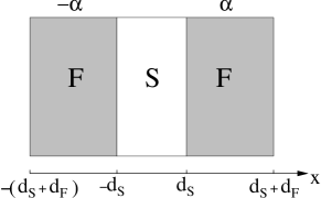
Figure 8: Trilayer geometry. The magnetization of the left (right) F layer makes an angle $\alpha$ ($-\alpha$) with the $z$-axis.

We want to demonstrate now that the triplet component with $S_{z}=\pm 1$ inevitably arises due to the overlap of the triplet components generated by the ferromagnetic layers in the $S$ layer. It is not difficult to understand why it should be so.

As we have seen in the previous section, each of the layers generates the triplet component with the zero total projection of the spin, $S_{z}=0,$ on the direction of the exchange field. If the magnetic moments of the layers are collinear to each other (parallel or antiparallel), the total projection remains zero. However, if the moments of the ferromagnetic layers are not collinear the superposition of the triplet components coming from the different layers should have all possible projections of the total spin.

From this argument we can expect the generation of the triplet component with all projections of the total spin provided the thickness of the $S$ layer is not too large. Since the only relevant length in the superconductors is $\xi_{S}\approx\sqrt{D_{S}/\pi T_{c}}$, we assume that the thickness of the superconducting layer $S$ does not exceed this length.

Now we perform explicit calculations that support the qualitative conclusion about the generation of the triplet component with all projections of the total spin. We consider the diffusive case when the Usadel equation is applicable. This means that the condition

$$h\tau<<1$$ (51)

is assumed to be fulfilled ($\tau$ is the elastic scattering time).

The linearized Usadel equation in the $F$ region takes the form (see Appendix A)

$$\partial^{2}_{xx}\check{f}-\kappa_{\omega}^{2}\check{f}+\frac{i\kappa_{h}^{2}}{2}\left\{\hat{\tau}_{0}[\hat{\sigma}_{3},\check{f}]_{+}\cos\alpha\pm\hat{\tau}_{3}[\hat{\sigma}_{2},\check{f}]\sin\alpha\right\}=0\;,$$ (52)

where $\check{f}$ is a $4\times 4$ matrix (condensate function) which is assumed to be small and $[\hat{\sigma}_{3},\check{f}]_{+}=\hat{\sigma}_{3}.\check{f}+\check{f}.\hat{\sigma}_{3}$. The wave vectors $\kappa_{\omega}$ and $\kappa_{h}$ entering Eq. (52) have the form

$$\kappa_{\omega}^{2}=2|\omega|/D_{F}$$ (53)

and

$$\kappa_{h}^{2}=2h\mathrm{sgn}\omega/D_{F}$$ (54)

The magnetization vector  $\mathbf{M}$ lies in the ($y,z$)-plane and has the components: $\mathbf{M}=M\{0,\pm\sin\alpha,\cos\alpha\}$. The sign “$+$” (“$-$”) corresponds to the right (left) ${F}$ film. We consider here the simplest case of a highly transparent $S/F$ interface and temperatures close to the critical temperature of the superconducting transition $T_{c}$. In this case the  function $\check{f}$, being small, obeys a linear equation similar to Eq.(45)

$$(\partial^{2}\check{f}/\partial x^{2})-\kappa_{S}^{2}\check{f}=2i(\delta\breve{\Delta}/D_{S})g_{BCS}^{2}\;,$$ (55)

where $\kappa_{S}^{2}=2|\omega|/D_{S}$.

The boundary conditions at the $S/F$ interfaces are

$$\check{f}_{x=d_{S}+0} = \check{f}_{x=d_{S}-0}$$ (56)

$$\gamma(\partial\check{f}/\partial x)|_{F} = (\partial\check{f}/\partial x)|_{S}\;.$$ (57)

where $\gamma=\sigma_{F}/\sigma_{S}$ and $\sigma_{F}\left(\sigma_{S}\right)$ is the conductivity in the ferromagnet (superconductor).

The first condition, Eq. (56), corresponds to the continuity of the condensate function at the ${S/F}$ interface with a high transparency, whereas Eq (57) ensures the continuity of the current across the ${S/F}$ interface Volkov et al. (2003).

A solution for Eqs.(52-55) with the boundary conditions (56-57) can easily be found. The matrix $\check{f}$ can be represented as

$$\check{f}=i\hat{\tau}_{2}\otimes\hat{f}_{2}+i\hat{\tau}_{1}\otimes\hat{f}_{1}\;,$$ (58)

where

$$\hat{f}_{1}=b_{1}(x)\hat{\sigma}_{1},\text{ \ }\hat{f}_{2}=b_{3}(x)\hat{\sigma}_{3}+b_{0}(x)\hat{\sigma}_{0},$$ (59)

In the left $F$ layer the functions $b_{k}(x)$ are to be replaced by $\bar{b}_{k}(x).$ For simplicity we assume that the thickness of the $F$ films $d_{F}$ exceeds $\xi_{F}$ (the case of an arbitrary $d_{F}$ was analyzed by Bergeret et al. (2003)). Using the representation, Eqs. (58-59), we find the functions $b_{i}(x)$ and $\bar{b}_{i}(x)$. They are decaying exponential functions and can be written as

$$b_{k}(x)=b_{k}\exp(-\kappa(x-d_{S})),\text{ }\bar{b}_{k}(x)\text{ }=\bar{b}_{k}\exp(\kappa(x+d_{S}))$$ (60)

Substituting Eq.(60) into Eqs.(52)-(55), we obtain a set of linear equations for the coefficients $b_{k}.$ The condition for the existence of non-trivial solutions yields an equation for the eigenvalues $\kappa.$ This equation reads

$$(\kappa^{2}-\kappa_{\omega}^{2})[(\kappa^{2}-\kappa_{\omega}^{2})^{2}+\kappa_{h}^{4}]=0$$ (61)

Eq. (61) is of the sixth order and therefore has six solutions. Three of these solutions should be discarded because the corresponding to $b_{k}\left(x\right)$ grow when going away from the interface. The remaining three solutions of Eq. (61) give three different physical values of $\kappa$.

If the exchange energy $h$ is sufficiently large ($h>>\{T,\Delta\}$), the eigenvalues are

$$\kappa = \kappa_{\omega}$$ (62)

$$\kappa_{\pm} \approx (1\pm i)\kappa_{h}$$ (63)

We see that these solutions are completely different. The roots $\kappa_{\pm}$ proportional to $\kappa_{h}$ (cf. Eq. (54)), are very large and therefore the corresponding solutions $b_{k}\left(s\right)$ decay very fast (similar to the singlet component). This is the solution that exists for a homogeneous magnetization (collinear magnetization vectors).

In contrast, the value for $\kappa$ given by Eq. (62), is much smaller (see Eq. (53)) and corresponds to a slow decay of the superconducting correlations. The solutions corresponding to the root given by Eq.(62) describe a long-range penetration of the triplet component into the ferromagnetic region. For each root one can easily obtain relations between the coefficients $b_{k}(x)$. As a result, we obtain

$$b_{1}(x) = b_{\omega}e^{-\kappa_{\omega}(x-d_{S})}$$ (64)

$$\!\!\!\!\!\!\!\!\!\!\!\!-\sin\alpha\left[b_{3+}e^{-\kappa_{+}(x-d_{S})}-b_{3-}e^{-\kappa_{-}(x-d_{S})}\right]\;$$

$$b_{0}(x) = -\tan\alpha\cdot b_{\omega}e^{-\kappa_{\omega}(x-d_{S})}$$ (65)

$$\!\!\!\!\!\!\!\!\!\!\!\!-\cos\alpha\left[b_{3+}e^{-\kappa_{+}(x-d_{S})}-b_{3-}e^{-\kappa_{-}(x-d_{S})}\right]$$

and

$$b_{3}(x)=b_{3+}\exp(-\kappa_{+}(x-d_{S}))+b_{3+}\exp(-\kappa_{-}(x-d_{S}))$$ (66)

The function $b_{1}(x)$ is the amplitude of the triplet component penetrating into the $F$ region over a long distance of the order of $\kappa_{\omega}^{-1}\sim\xi_{N}.$ Its value as well as the values of the other functions $b_{k}(x)$ is found from the boundary conditions (56-57) at the $S/F$ interfaces.

What remains to be done is to match the solutions for the superconductor and the ferromagnets at the interfaces between them. The solution for the superconductor satisfies Eq.(55) and can be written as

$$f_{3}(x) = \Delta/iE_{\omega}+a_{3}\cosh(\kappa_{S}x)$$ (67)

$$f_{0}(x) = a_{0}\cosh(\kappa_{S}x)$$ (68)

$$f_{1}(x) = a_{1}\sinh(\kappa_{S}x)\;,$$ (69)

where $E_{\omega}=\sqrt{\omega^{2}+\Delta^{2}}$.

Matching these solutions with Eqs. (64-66) at the $S/F$ interfaces we obtain the coefficients $b_{k}$ and $\bar{b}_{k}$ as well as $a_{k}$. Note that $b_{3\pm}=$ $\bar{b}_{3\pm}$ and $b_{\omega}=$ $-\bar{b}_{\omega}.$ Although the solution can be found for arbitrary parameters entering the equations, we present here for brevity the expressions for $b_{3\pm}$ and $b_{\omega}$ in some limiting cases only.

Let us consider first the case when the parameter $\gamma\kappa_{h}/\kappa_{S}$  is small, that is, we assume the condition

$$\gamma\kappa_{h}/\kappa_{S}\approx\frac{\nu_{F}}{\nu_{S}}\sqrt{\frac{D_{F}h}{D_{S}\pi T_{c}}}<<1$$ (70)

to be fulfilled.

Here $\nu_{F,S}$ is the density of states in the ferromagnet and superconductor, respectively (in the quasiclassical approximation the DOS for electrons with spin up and spin down is nearly the same: $h<<\epsilon_{F}$). The condition, Eq. (70), can be fulfilled in the limit $D_{F}<<D_{S}$. Taking, for example, $\nu_{F}\approx\nu_{S},$ $l_{F}\approx 30$ Å and $l_{S}\approx 300$ Å, we find that $h$ should be smaller than $30T_{c}$.

In this limit the coefficients $b_{1,3\pm}$ and $a_{1}$ can be written in a rather simple form

$$b_{\omega}\approx-\frac{2\Delta}{E_{\omega}}(\frac{\gamma\kappa_{h}}{\kappa_{S}})\frac{\sin\alpha\cos^{2}\alpha}{\sinh(2\Theta_{S})},$$ (71)

$$b_{3+}\approx b_{3-}\approx\frac{\Delta}{2i\xi_{\omega}},$$ (72)

$$a_{3}=-\frac{\Delta}{iE_{\omega}}\frac{\gamma\kappa_{h}}{\kappa_{S}}\frac{1}{\sinh(2\Theta_{S})},$$ (73)

where  $\Theta=\kappa_{S}d_{S}.$

As follows from the first of these equations, Eq. (72), the correction to the bulk BCS solution for the singlet component is small in this approximation and this justifies our approach.

At the $S/F$ interface the amplitude of the triplet component $b_{\omega}$ is small in comparison with the magnitude of the singlet one $b_{3+}$ . However the triplet component decays over a long distance $\xi_{N}$ while the singlet one vanishes at distances exceeding the short length $\xi_{F}$. The amplitudes $b_{\omega}$ and $b_{3\pm}$ become comparable if the parameter $\gamma\kappa_{h}/\kappa_{S}$ is of the order of unity.

It follows also from Eq.(71) that the amplitude of the triplet component $b_{\omega}$ is zero in the case of collinear vectors of magnetization, i.e. at $\alpha=0$ or $\alpha=\pi/2$. It reaches the maximum at the angle $\alpha_{m}$ for which $\sin\alpha_{m}=1/\sqrt{3}$. Therefore the maximum angle-dependent factor in Eq.(71) is $\sin\alpha_{m}\cos^{2}\alpha_{m}=2/3\sqrt{3}\approx 0.385.$

One can see from Eq.(71) that $b_{\omega}$ becomes exponentially small if the thickness $d_{S\text{ }}$of the $S$ films significantly exceeds the coherence length $\xi_{S}\approx\sqrt{D_{S}/\pi T_{c}}$. This means that in order to have a considerable penetration of the superconducting condensate into the ferromagnet one should not make the superconducting layer too thick.

On the other hand, if the thickness $d_{S}$ is too small the critical temperature $T_{c}$ is suppressed. In order to avoid this suppression one has to use, for instance, an $F/S/F$ structure with a small width of the $F$ films. Similar systems were considered by Beckmann et al. (2004), where non-local effects of Andreev reflections in a $S/F$ nanostructure were studied .

Another limiting case that allows a comparatively simple solution is the limit of small angles $\alpha$ Volkov et al. (2003) but an arbitrary parameter $\gamma\kappa_{h}/\kappa_{S}$, Eq. (70). At small angles $\alpha$ the amplitudes of the triplet and singlet component are given by the following formulae

$$b_{\omega}\approx-\frac{\Delta}{E_{\omega}}\frac{\sin\alpha(\gamma\kappa_{h}/\kappa_{S})\tanh\Theta_{S}}{\cosh^{2}\Theta_{S}|\tanh\Theta_{S}+(\gamma\kappa_{h}/\kappa_{S})|^{2}(1+(\gamma\kappa_{h}/\kappa_{S})\tanh\Theta_{S})},$$ (74)

$$b_{3\pm}\approx\frac{\Delta}{2iE_{\omega}}\frac{1}{1+(\gamma\kappa_{\pm}/\kappa_{S})\tanh\Theta_{S}},$$ (75)

One can see from Eqs. (74-75) that, provided the parameter given by Eq. (70) is not small and $\alpha,|\Theta_{S}|\sim 1$, the amplitudes $b_{\omega}$ and $b_{3\pm}$ are again comparable with each other.

The amplitudes of the triplet and singlet components were calculated by Bergeret et al. (2003) in a more general case of an arbitrary $S/F$ interface transparency and a finite thickness of the $F$ films.

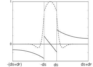
Figure 9: The spatial dependence of $\mathrm{Im}$(SC) (dashed line) and the long-range part of $\mathrm{Re}$(TC) (solid line). We have chosen $\sigma_{F}/\sigma_{S}=0.2$, $h/T_{C}=50$, $\sigma_{F}R_{b}/\xi_{F}=0.05$, $d_{F}\sqrt{T_{C}/D_{S}}=2$, $d_{S}\sqrt{T_{C}/D_{S}}=0.4$ and $\alpha=\pi/4$. The discontinuity of the TC at the S/F interface is because the short-range part is not shown in this figure. Taken from Bergeret, Volkov, and Efetov (2003)

In FIG. 9 we plot the spatial dependence of the triplet (TC) and singlet (SC) components in a $F/S/F$ structure. It is seen from this figure that, as expected, the triplet component decays slowly, whereas the singlet component decays fast over the short length $\xi_{h}$. For this reason, in a multilayered $S/F$ structure with a varying direction of the magnetization vector $\mathbf{M}$ and thick $F$ layers ($\xi_{h}<<d_{F}$) a Josephson-like coupling between neighboring layers can be realized via the odd triplet component. In this case the in-plane superconductivity is caused by both triplet and singlet components. Properties of such S/F multilayered structures will be discussed in the next chapter.

Let us mention an important fact. The quasiclassical Green’s function $\check{g}(\vartheta)$ in the diffusive case can be expanded in spherical harmonics. In the present approach, only the first two terms of this expansion are taken into account such that

$$\;\check{g}=\check{g}_{sym}+\check{g}_{as}\cos\vartheta$$ (76)

where $\vartheta$ is the angle between the momentum $p$ and the $x$-axis, and $\check{g}_{as}=-l\check{g}_{sym}\partial\check{g}_{sym}/\partial x$ is the antisymmetric part of $\check{g}(\vartheta)$ and $\check{g}_{sym}$ is the isotropic part of $\check{g}(\vartheta)$, which does not depend on $\vartheta$. The antisymmetric part of $\check{g}$ determines the electric current in the system.

Higher order terms in the expansion of $\check{g}$ are small in the diffusive limit and can be neglected. In the case of a weak proximity effect the antisymmetric part of the condensate function in the $F$ region can be written as

$$\;\check{f}_{as}\cos\vartheta\approx-l\hat{\tau}_{3}\otimes\hat{\sigma}_{0}\mbox{${\rm sgn}$}\omega\partial\check{f}_{sym}/\partial x\cos\vartheta\;.$$ (77)

This expression follows from the fact that $\check{g}_{0}\approx-\hat{\tau}_{3}\otimes\hat{\sigma}_{0}\mbox{${\rm sgn}$}\omega$ (corrections to $\check{g}_{0}$ are proportional to $\;\check{f}_{0}^{2}$). Eq. (77) holds for both the singlet and triplet components.

As we have clarified previously, the symmetric part $\check{f}_{0}$ is an odd function of $\omega$. Thus, according to Eq.(75) the antisymmetric part is an even function of $\omega$ so that the total condensate function $\check{f}=\check{f}_{0}+\check{f}_{1}\cos\vartheta$ is neither odd nor even function of $\omega$. However, in the diffusive limit it is still legitimate to speak about the odd superconductivity since the symmetric part is much larger than antisymmetric part of $\check{f}$.

If the parameter $h\tau$ is not small, i.e. the system is not diffusive, the symmetric and antisymmetric parts are comparable, and one cannot speak of the odd superconductivity. All this distinguishes the superconductivity in $S/F$ structures from the odd superconductivity suggested by Berezinskii (1975) who assumed that the order parameter $\Delta(\omega)$ was an odd function of $\omega$. In our discussion it is assumed that the order parameter $\Delta$ is an $\omega-$ independent quantity and it is determined by the singlet component of the condensate function $\check{f}_{0}$.

III.3.2 Domain wall at the S/F interface

In the previous section we have seen how the generation of the triplet component takes place. The appearance of this component leads to long range effects in a structure where the angle between the directions of magnetization in the different layers can be changed experimentally. This is an example of a situation when the long range triplet component of the superconducting condensate can be produced under artificial experimental conditions.

In this section we show that the conditions under which the triplet long range superconducting correlations occur are considerably more general. It is well known that the magnetization of any ferromagnet can be quite inhomogeneous due to the presence of domain walls. They are especially probable near interfaces between the ferromagnets and other materials. Therefore, making an interface between the ferromagnets and superconductors one produces almost inevitably domain walls, and one should take special care to get rid off them.

Figure 10: S/F structure with a domain wall in the region $0<x<w$. In this region $\alpha=Qx$, where $Q$ is the wave vector which describes the spiral structure of the domain wall. For $x>w$ it is assumed that the magnetization is homogeneous, i.e. $\alpha_{w}\equiv\alpha(x>w)=Qw$.

In this section we consider a domain wall like structure and show that it will also lead to the triplet long range correlations. This structure is shown schematically in FIG. 10. It consists of a $S/F$ bilayer with a non-homogeneous magnetization in the $F$ layer. We assume for simplicity that the magnetization vector $\mathbf{M}=M(0,\sin\alpha(x),\cos\alpha(x))$ rotates in the $F$ film starting from the $S/F$ interface ($x=0$) and the rotation angle has a simple piece-wise $x$-dependence

$$\alpha(x)=\left\{\begin{array}[]{l}Qx,\text{ \ }0<x<w\\ \alpha_{w}=Qw,\text{ \ }w<x\end{array}\right.$$ (78)

This form  means that the $\mathbf{M}$ vector is aligned parallel to the $z$-axis at the $S/F$ interface and rotates by the angle $\alpha_{w}$($=\alpha(w)$) over the length $w$ ($w$ may be the width of a domain wall). At $x>w$ the orientation of the vector $\mathbf{M}$ is fixed.

We calculate the condensate function in the $F$ region and show that it contains the long range triplet component (LRTC). As in the preceding section, we assume that the condensate function in the $F$ region is small. The smallness of $\check{f}$ in this case is either due to a mismatch of the Fermi velocities in the superconductor and ferromagnet or due to a possible potential barrier at the $S/F$ interface. In such cases the transparency of the interface is small and only a small portion of the superconducting electrons penetrates the ferromagnet.

Due to the smallness of the transparency of the interface  the function $\check{f}$ can experience a jump at the $S/F$ interface, which contrasts the preceding case. The boundary condition for the $4\times 4$ matrix $\check{f}$ has the same form as in Eq.(27)

$$\;\gamma_{F}\partial_{x}\check{f}=-\check{f}_{S}$$ (79)

The function $\check{f}_{S}$ on the right-had side is the condensate matrix Green’s function in the superconductor that, in the limit considered here, should be close to the bulk solution

$$\;\check{f}_{S}\;=f_{BCS}i\hat{\tau}_{2}\otimes\hat{\sigma}_{3}$$ (80)

We have to solve again Eq.(52) with the boundary conditions (79). Therefore we assume that the domain wall thickness $w$ is larger than the mean free path $l\$and the condition, Eq. (51) is fulfilled (dirty limit). This case was analyzed by Bergeret et al. (2001b). Another case of a thin domain wall ($w<l$) was considered by Kadigrobov et al. (2001).

The problem of finding the condensate functions in the case of the magnetization varying continuously in space is more difficult than the previous one because the angle $\alpha$ depends now on $x$. However, one can use a trick that helps to solve the problem, namely, we exclude the dependence $\alpha(x)$ introducing a new matrix $\check{f}_{n}$ related to $\check{f}$ via an unitary transformation (a rotation in the particle-hole and spin-space)

$$\;\check{f}\;=\check{U}.\check{f}_{n}.\check{U}^{+}$$ (81)

where $\check{U}=\exp(i\hat{\tau}_{3}\otimes\hat{\sigma}_{1}\alpha(x)/2).$

Performing this transformation we obtain instead of Eq.(52) a new equation

$$\;(\partial^{2}_{xx}-Q^{2}/2)\check{f}_{n} - \kappa_{\omega}^{2}\check{f}_{n}\;+i\kappa_{h}^{2}[\hat{\sigma}_{3},\check{f}_{n}]_{+}$$

$$-\frac{Q^{2}}{2}(\hat{\sigma}_{1}\check{f}_{n}\hat{\sigma}_{1}) + iQ\hat{\tau}_{3}[\hat{\sigma}_{1},\partial_{x}\check{f}_{n}]_{+}=0$$ (82)

Correspondingly, the boundary condition, Eq. (79), takes the form

$$\;\gamma_{F}\{(Q/2)i\hat{\tau}_{3}[\hat{\sigma}_{1,}\check{f}_{n}]_{+}+\partial\check{f}_{n}\;/\partial x\}=-\check{f}_{s}$$ (83)

Eq.(82) complemented by this boundary condition has to be solved in the region $0<x<w$. In the region $w<x$ one needs to solve Eq.(52) with $Q=0$. Both the solutions should be matched at $x=w$ under the assumption that there is no barrier at this point. Therefore, the matrix $\check{f}_{n}$ and its ”generalized” derivative should be continuous at $x=w$

$$\check{f}_{n}\mid_{x=w-0} = \check{f}_{n}\mid_{x=w+0}$$ (84)

$$\frac{Q}{2}i\hat{\tau}_{3}[\hat{\sigma}_{1,}\check{f}_{n}]_{+} + \partial_{x}\check{f}_{n}\mid_{x=w-0}=\partial_{x}\check{f}_{n}\mid_{x=w+0}$$ (85)

In this case the solution has the same structure as Eq.(58)  but small changes should be done. The eigenvalues $\kappa$  obey the equation

$$[(\kappa^{2}-Q^{2}-\kappa_{\omega}^{2})^{2}+4Q^{2}\kappa_{\omega}^{2}](\kappa^{2}-\kappa_{\omega}^{2})+\kappa_{h}^{4}[\kappa^{2}-Q^{2}-\kappa_{\omega}^{2}]=0$$ (86)

where $\kappa_{\omega,h}^{2}$ are determined in Eqs.(53,54). The eigenvalue given by Eq. (62) changes. Now it is equal to

$$\;\kappa_{Q}^{2}=Q^{2}+\kappa_{\omega}^{2}\;,$$ (87)

while the eigenvalues $\kappa_{\pm},$ Eq. (63), remain unchanged provided the condition

$$\;Q,\kappa_{\omega}<<\kappa_{h}$$ (88)

is fulfilled.

In the opposite limit of large $Q>>\kappa_{h}$, the eigenvalues $\kappa_{\pm}$ take the form

$$\;\kappa_{\pm}=\pm iQ[1\mp i\kappa_{h}^{2}/\sqrt{2}Q^{2}],$$ (89)

Thus, in this limit $\kappa_{\pm}$ is imaginary in the main approximation, which means that the function $\check{f}_{n}(x)$ oscillates fast in space with the period $2\pi/Q$. In this case the eigenvalues (87) change also and have the form

$$\kappa^{2}=\kappa_{\omega}^{2}+\frac{\kappa_{h}^{4}}{Q^{2}}$$ (90)

Therefore the limit of a very fast rotating magnetization ($\kappa_{h}/Q\rightarrow 0$) is analogous to the case of a normal metal, i.e. when the condensate penetrates the ferromagnet over the length $\kappa_{\omega}^{-1}\sim\sqrt{D_{F}/2\pi T}$ which is the characteristic penetration length of the condensate in a S/N system.

More interesting and realistic is the opposite limit when the condition (88) is fulfilled and the long-range penetration of the triplet component into the ferromagnet becomes possible.

In the limit of large $\kappa_{h}$, (Eq. (88)), the singlet component penetrates the ferromagnet over a short length of the order $\xi_{h}=1/\kappa_{h}$ while the LRTC penetrates over the length $\sim 1/\kappa_{Q}$. As follows from Eq. (87), this penetration length is about $1/Q$ (provided $w/\alpha_{w}$ is smaller than the length $\xi_{N}$).

Now let us find the amplitude of the LRTC. The solution for Eq.(82) in the interval $0<x<w$ is determined by Eqs.(58, 59) with the functions $b_{i}\left(x\right)$, $i=0,1,3$ given by the following formulae

$$b_{1}(x)=b_{Q}\exp(\kappa_{Q}x)+\bar{b}_{Q}\exp(-\kappa_{Q}x)\;$$ (91)

$$b_{0}(x)=-b_{3+}\exp(-\kappa_{+}x)+b_{3-}\exp(-\kappa_{-}x)\;$$ (92)

and

$$b_{3}(x)=b_{3+}\exp(-\kappa_{+}x)+b_{3-}\exp(-\kappa_{-}x)\;$$ (93)

In the region $w<x$ the solution for the condensate function $\check{f}_{n}$ takes the form

$$\;\;\check{f}_{n}\;=i\hat{\tau}_{1}\otimes\hat{\sigma}_{1}c_{\omega}\exp(-\kappa_{\omega}(x-w))$$ (94)

where $c_{\omega}$ is a coefficient that has to be found by matching the solutions  at  $x=w$.

Terms of the order of $Q/\kappa_{h}$ are small and they are omitted now.

Then we find from the matching conditions at the $S/F$ interface, Eq. (85), the following relations for the coefficients

$$b_{3\pm}=\frac{f_{BCS}}{2\gamma_{F}\kappa_{\pm}}$$ (95)

and

$$b_{Q}=-\bar{b}_{Q}=(Q/\kappa_{Q})(b_{3+}-b_{3-})$$ (96)

(the parameter $\gamma_{F}$ given by Eq. (79))

One can see from the above equations  that the condensate function $|\check{f}|$ is small provided parameter $|\gamma_{F}\kappa_{\pm}|$ is large. It follows from Eq.(96) that the amplitude of the LRTC, $b_{Q}$, is not zero only if the magnetization is nonhomogeneous, i.e., $Q\neq 0.$

Matching the solutions (91-94) at $x=w$, we find for the amplitude of the LRTC

$$\;\;c_{\omega}=-\frac{if_{BCS}}{2\gamma_{F}}[\frac{Q}{\kappa_{Q}\sinh\alpha_{w}+\kappa_{\omega}\cosh\alpha_{w}}](\frac{h\mathrm{sgn}\omega/D_{F}}{|\kappa_{+}|^{2}\mathrm{Re}\kappa_{+}})$$ (97)

where $\alpha_{w}=Qw$ is the total angle of the magnetization rotation. As it has been mentioned, the amplitude of the LRTC is an odd function of $\omega$.

As one can see from the last expression the amplitude $c_{\omega}$ increases from zero when increasing $Q$, reaches a maximum at $Q_{max}$ corresponding a certain angle $\alpha_{max}$ and then exponentially decreases at $\alpha_{w}>>$ $\alpha_{max}.$

The maximum of $c_{\omega}$  is achieved at

$$\;\alpha_{max}=(w\kappa_{\omega})\sqrt{\sqrt{5}-1}/\sqrt{2}\approx 0.786(w\kappa_{\omega})\;,$$ (98)

At $\alpha_{w}=\alpha_{max}$  the ratio in the square brackets in Eq.(97) is equal to $\approx 0.68$ . This means that the amplitude of the LRTC is of the order of the singlet component at the $S/F$ interface. The width $w$ should not be too small because in deriving the expression for $c_{Q}$ we assumed the condition $w>>\xi_{h}.$

In FIG. 11 we represented the dependence of $\left|c_{\omega}\right|$ on $\alpha_{w}$ for a fixed $w$. The spatial dependence of the LRTC and the singlet component is shown in FIG. 12. It is seen that for the parameters chosen the LRTC is larger than the singlet component and decays much slower with increasing the distance $x$.

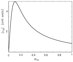
Figure 11: Dependence of the amplitude of the triplet component on $\alpha_{w}=Qw$. We have chosen $w\kappa_{\omega}=0.01$.

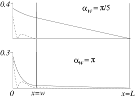
Figure 12: Spatial dependence of the amplitudes of the singlet (dashed line) and triplet (solid line) components of the condensate function in the F wire for different values of $\alpha_{w}$. Here $w=L/5$, $\epsilon=E_{T}$ and $h/E_{T}=400$. $E_{T}=D/L^{2}$ is the Thouless energy (From Bergeret, Volkov, and Efetov (2001a)).

If the magnetization vector $\mathbf{M}$ rotates by the angle $\pi$ (a domain wall) over a small length $w$ so that $Q\sim\pi/w>>\kappa_{w}$, then the ratio in brackets in Eq.(97) is equal to

$$\;\;(\frac{Q}{\kappa_{Q}\sinh\alpha_{w}+\kappa_{\omega}\cosh\alpha_{w}})\approx Q/(Q\sinh\pi)\approx 0.087$$ (99)

which shows that the amplitude of the LRTC in this case is smaller than the amplitude of the singlet component.

We can conclude from this analysis that in order to get a large LRTC, a small total angle of the rotation of the magnetization vector is more preferable.

The amplitude of the condensate function calculated here enters different physical quantities. In section III.4 we discuss how the long-range penetration of the triplet component into the ferromagnet affects transport properties of $F/S$ structures.

It is interesting to note that the type of magnetic structure discussed in this section differs drastically from the one in the case of an in-plane rotating magnetization. The latter was considered recently by Champel and Eschrig (2005a, b). It was assumed that the magnetization vector $M_{F}$ was parallel to the S/F interface and rotates; that is, it has the form $M_{F}=M_{0}\{0,\sin(Qy),\cos(Qy)\}$ (the x-axis is normal to the S/F interface plane). As shown by Champel and Eschrig (2005b), the odd triplet component arises also in this case but it penetrates into the ferromagnetic region over a short distance of the order of $\xi_{h}$.

III.3.3 Spin-active Interfaces

In almost all papers containing discussions of the $S/F$ structures it is assumed that the $S/F$ interface is spin-inactive, i.e. the spin of an electron does not change when the electron goes through the interface.

Although in many cases it is really so , one can imagine another situation when the spin of an electron passing through the interface changes. One can consider a region with a domain wall at the interface also as a “ spin-active interface” provided the width $w$ of the domain wall is very small but the product $Qw$ is of the order unity. As we have seen in section III.3.2, at such type of interfaces the triplet condensate arises.

Boundary conditions at spin-active $S/F$ interfaces for the quasiclassical Green’s functions were derived in a number of publications Millis et al. (1988); Kopu et al. (2004) and were used in studying different problems. Kulic and Endres (2000) employed these boundary conditions in the study of a system similar to the one shown in FIG. 8. Contrary to Bergeret et al. (2003), they assumed that the ferromagnets $F$ are insulators so that the condensate does not penetrate them. Nevertheless, the calculated critical temperature $T_{c}$ of the superconducting transition depends on the mutual orientation of the magnetization $M_{F}$ in the ferromagnets. In accordance with Baladie and Buzdin (2003); Tagirov (1998); Fominov et al. (2002) where metallic ferromagnets were considered in a $F/S/F$ structure, Kulic and Endres found that the critical temperature $T_{c}$ was maximal for the antiparallel magnetization orientation. If the directions of magnetization vector $M_{F}$ are perpendicular to each other, a triplet component also arises in the superconductor. The authors considered a clean case only, so that the influence of impurity scattering on the triplet component remained unclear.

According to Huertas-Hernando et al. (2002) a spin-active N/F interface plays an important role in the absolute spin-valve effect which can take place in a S/N/F mesoscopic structure. The authors considered a structure with a thin normal metal layer (N) and a ferromagnetic insulator F. The DOS variation in a conventional superconductor which is in contact with a ferromagnetic insulator was analyzed by Tokuyasu et al. (1988).

Eschrig et al. (2003) considered a clean $S/F/S$  Josephson junction in which the ferromagnet $F$  was a half metal so that the electrons with only one spin orientation (say the spin-up $\uparrow$ electrons) existed in the ferromagnet. In this case only the triplet component corresponding to the condensate function $<\psi_{\uparrow}\psi_{\uparrow}>$  may penetrate the ferromagnet. Assuming the p-wave triplet condensate function, the authors have calculated the critical Josephson current $I_{c}$ . They showed that the $\pi-$  state (negative critical current $I_{c}$ ) is possible in this junction. The dc Josephson effect in a junction consisting of two superconductors and a spin-active interface between them was analyzed by Fogelström (2000).

It would be of interest to analyze the influence of impurities on the critical current in such type of Josephson junctions because, as we noted, in a clean case the singlet component can penetrate the ferromagnet (not a half metal) over a large distance.

III.4 Long-range proximity effect

In the last decade transport properties of mesoscopic superconductor/normal metal $S/N$ structures were intensively studied (see for example the review articles by Beenakker (1997); Lambert and Raimondi (1998) and references therein). In the course of these studies many interesting phenomena have been discovered. Among them is a non-monotonic voltage and temperature dependence of the conductance in $S/N$ mesoscopic structures, i.e. structures whose dimensions are less than the phase coherence length $L_{\varphi}$ and the inelastic scattering length $l_{\varepsilon}$. This means that the resistance $R$ of a $S/N$ structure changes non-monotonically when the temperature decreases below the critical temperature $T_{c}$.

This complicated behavior is due to the fact that there are two contributions to the resistance in such systems: the one coming from the $S/N$ interface resistance and the resistance of the normal wire itself. The experimentally observed changes of the resistance can be both positive ($\delta R>0$) and negative ($\delta R<0$) Quirion et al. (2002); Shapira et al. (2000). The increase or decrease of the resistance $R$ depends, in particular, on the interface resistance $R_{S/N}$. If the latter is very small, the resistance of the $S/N$ structure is determined mainly by the resistance of the $N$ wire $R_{N}$. This resistance decreases with decreasing the temperature $T$, reaches a minimum at a temperature of the order of the Thouless energy $D_{N}/L_{N}^{2}$, and increases again returning to the value in the normal state $R_{N}(T_{c})$ at low $T$, where $D_{N}$ is the diffusion coefficient and $L_{N}$ is the length of the $N$ wire. This is the so called re-entrant behavior observed in many experiments Gubankov and Margolin (1979); Pothier et al. (1994); Dimoulas et al. (1995); Petrashov et al. (1995); Charlat et al. (1996); Chien and Chandrasekhar (1999); Shapira et al. (2000).

Theoretical explanations for the non-monotonic behavior of the resistance variation as a function of the temperature $T$ or voltage $V$ in $S/N$ structures have been presented by Artemenko et al. (1979); Volkov et al. (1993); Nazarov and Stoof (1996); Volkov et al. (1996); Golubov et al. (1997); Shapira et al. (2000). Such a variation of the resistance of the normal metal wire can be explained in terms of the proximity effect that leads to the penetration of the condensate into the ${N}$ wire. Due to this penetration there are two types of contributions to the conductance $G_{N}$ Volkov and Pavlovskii (1996); Golubov et al. (1997). One of them reduces the DOS in the $N$ wire and therefore reduces the conductance $G_{N}.$ The  other term, similar to the Maki-Thompson term Golubov et al. (1997); Volkov and Pavlovskii (1996), leads to an increase of the conductance of the $N$ wire.

In principle, the magnitude of the conductance variation $\delta G_{N}$ may be comparable with the conductance $G_{N}$. So, there are no doubts that the proximity effect plays a very important role in many experiments on $S/N$ structures.

Recently, similar investigations have been carried out also on mesoscopic $F/S$ structures in which ferromagnets ($F$) were used instead of normal (nonmagnetic) metals. According to our previous discussion, the depth of the condensate penetration into an impure ferromagnet equals $\xi_{F}=\sqrt{\hbar D/h}$. This length is extremely short ($5-50$Å) for strong ferromagnets like $Fe$ or $Ni$. Therefore one might expect that the influence of the proximity effect on the transport properties of such structures should be negligibly small.

It was a great surprise that experiments carried out recently on $F/S$ structures showed that the resistance variation $\delta R$ were quite visible (varying from about $1$ to $10\%$) when decreasing the temperature below $T_{c}$ Lawrence and Giordano (1996a, b); Petrashov et al. (1999); Aumentado and Chandrasekhar (2001); Giroud et al. (1998). For example in the experiments by Lawrence and Giordano (1996a, b), where an $Sn/Ni$ structure was studied, the effective condensate penetration length estimated from the measured resistance was about $400$Å. This quantity exceeds $\xi_{F}$ by order of magnitude. Similar results have been obtained by Giroud et al. (1998) on $Co/Al$ structures, by Petrashov et al. (1999) on a $Ni/Al$ structures and by Aumentado and Chandrasekhar (2001) on $Ni/Al$ structures.

It is worth mentioning that the change of the  resistance was both positive and negative. In some experiments the variation $\delta R_{F}$ was related to a change of the interface resistance Aumentado and Chandrasekhar (2001), whereas in others Lawrence and Giordano (1996a, b); Petrashov et al. (1999); Giroud et al. (1998) to the resistance variation of the ferromagnetic wire $\delta R_{F}$.

Figure 13: Reduction of the resistance of a Ni wire attached to a superconductor(Al). Adapted from Petrashov et al. (1999).

In FIG. 13 we show the temperature dependence of the resistance of a $Ni$ wire attached to an $Al$ bank measured by Petrashov et al. (1999). According to estimates of $\xi_{F}$ performed in this experiments, the observed $\delta R_{F}$ is by two orders of magnitude larger than it might be expected from the conventional theory of  $S/F$ the contacts. Therefore these results cannot be explained in terms of the penetration of the singlet component.

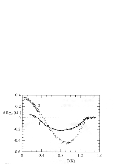
Figure 14: Temperature dependence of the resistance of a Co wire attached to a superconductor (Al) measured by Giroud et al. (1998). Note that at low temperatures the authors observed a reentrance behavior.

In FIG. 14  we show similar data from the  experiment on ${Co/Al}$ structures performed by Giroud et al. (1998). In this experiments a reentrance behavior of $\delta R$ was observed. In the limit of very low temperatures $T\rightarrow 0$ the resistance was even larger than in the normal state.

The final explanation of this effect remains until now unclear. However, the long range proximity effects considered in the previous sections may definitely contribute to the conductance variation. In order to support this point of view we analyze qualitatively the changes of the conductance due to the LRTC penetration into the ferromagnet and demonstrate that the LRTC may lead to the conductance variation comparable with that observed in the experiments.

However, before presenting these calculations it is reasonable to understand if one can explain the experiments in a more simple way. Actually, the resistance of the $S/F$ structures has been analyzed in many theoretical works. For example, de Jong and Beenakker (1994); Golubov (1999); Belzig et al. (2000) analyzed a ballistic $S/F$ contact. It was shown that at zero exchange field ($h=0$), the contact conductance $G_{F/S}$ is twice as large as its conductance $G_{F/N}$ in the normal state (above $T_{c}$), as it should be. This agrees with a conductance in a $N/S$ ballistic contact according to theoretical predictions. At the same time, it drops to zero at $h=E_{F},$ where $E_{F}$ is the Fermi energy.

The conductance of a diffusive point contact $G_{F/S}$ has been calculated by Golubov (1999) who showed that $G_{F/S}$ was always smaller than the conductance $G_{F/N}$ in the normal state. In the case of a mixed conductivity mechanism (partly diffusive and partly ballistic) the conductance $G_{F/S}$ has been calculated by Belzig et al. (2000). According to their calculations it can be both larger or smaller than the conductance in the normal state $G_{F/N}$.

The resistance $R_{F}$ of a ferromagnetic wire attached to a superconductor was calculated by Falko et al. (1999); Jedema et al. (1999); Bergeret et al. (2002a) and let us shortly describe what happens in such a system.

The proximity effect was neglected in these works but a difference in the conductivities $\sigma_{\uparrow\downarrow}$ for spin-up and down electrons was taken into account. The change of the conductance (or resistance) $\delta G_{F}$ is caused by a different form of the distribution functions below and above $T_{c}$ because of Andreev reflections.

The conductance $G_{F}(T_{c})$ of the $F$ wire in the normal state ($T>T_{c}$) is given by the simple expression

$$\;\;G_{F}(T_{c})=G_{\uparrow}+G_{\downarrow}\;,$$ (100)

where $G_{\uparrow\downarrow}=\sigma_{\uparrow\downarrow}L_{F}A,$ $L_{F}$ and $A$ are the length and cross-section area of the $F$ wire.

This means that the total conductance is the sum of the conductances of the spin-up and down channels. In this case not only the electric current but also the spin current is not zero. It turns out that  below $T_{c}$ ($T<T_{c}$) the conductance decreases and at zero temperature it is equal to

$$\;\;G_{F}(0)=4G_{\uparrow}G_{\downarrow}/(G_{\uparrow}+G_{\downarrow})$$ (101)

Eq. (101) shows  that the zero-temperature conductance $G_{F}(0)$ for the system considered is smaller than the normal state conductance $G_{F}(T_{c}).$

It is possible to obtain the explicit formulae not only in the limiting cases, Eq. (100, 101), but also to describe the system at arbitrary temperatures. The general formula for the conductance of the $F$ wire can be written as

$$\;\;G_{F}(T)=G_{F}(0)\tanh(\Delta/2T)+G_{F}(T_{c})(1-\tanh(\Delta/2T))$$ (102)

Eqs. (100) and (101) can be obtained from Eq. (102) by putting $\Delta$ or $T$ to zero. Eqs.(100-102) are valid provided the length $L_{F}$ satisfies the condition

$$l_{\uparrow\downarrow}<L_{F}<L_{SO},L_{in}\;,$$ (103)

where $\;l_{\uparrow\downarrow}$ is the mean free path of spin-up and spin-down electrons,while $L_{SO}$ and $L_{in}$ are the spin-orbit and inelastic relaxation length, respectively.

The resistance of multiterminal $S/F$  structures was calculated by Mélin (2001); Mélin and Peysson (2003); Mélin and Feinberg (2004) on the basis of the tunnel Hamiltonian method. The influence of superconducting contacts on giant magnetoresistance in multilayered structures was studied by Taddei et al. (2001). Tkachov et al. (2002) studied an enhancement of Andreev reflection at the S/F interface due to inelastic magnon-assisted scattering.

One can conclude from the works listed above that neglecting the penetration of the LRTC into the $F$ wire an increase in the conductance $G_{F}$ cannot be explained. Therefore,  let us discuss the consequences of the LRTC penetration into the ferromagnetic wire. In order to avoid the consideration of the $S/F$ interface contribution to the total resistance, we consider a cross geometry (see FIG. 15) and assume that the resistance of the interface between the $F$ wire and $F$ reservoirs is negligible. Such a geometry was used, for example, in the experiments by Petrashov et al. (1995). The structure under consideration consists of two $F$ wires attached to the $F$ and $S$ reservoirs. We assume that there is a significant mismatch between parameters of the superconductor and ferromagnet so that the condensate amplitude induced in $F$ is small and is determined by Eqs.(74) or (97).

Figure 15: The cross geometry used to measured the changes of the resistance of a F wire due to the proximity effect.

According to our results obtained previously the long range proximity effect is possible provided there is a domain wall near the interface between the superconductor and ferromagnet and we assume that this is the case for the setup shown in FIG. 15. Another possibility to generate the triplet condensate would be to attach to the superconductor   an additional ferromagnet with a non-collinear magnetization.

The conductance can be found on the basis of a general formula for the current (see for example the book by Kopnin (2001) and Appendix A)

$$I=(1/16e)(L_{y}L_{z})\sigma_{F}\mathrm{Tr}\hat{\sigma}_{0}\otimes\hat{\tau}_{3}\circ\int\mathrm{d}\epsilon[\check{g}^{R}\partial_{x}\check{g}^{K}+\check{g}^{K}\partial_{x}\check{g}^{A}]$$ (104)

where $\sigma_{F}$ is the conductivity of the $F$ wire in the normal state.

The matrix Green’s function $\check{g}^{K}=\check{g}^{R}\check{F}-\check{F}$ $\check{g}^{A}$ is the Keldysh function related to a matrix distribution function $\check{F}$. The distribution function consists of two parts, namely, one of them is symmetric with respect to the energy $\epsilon$, the  other one is antisymmetric in $\epsilon$ and determines the dissipative current.

In the limit of a weak proximity effect the retarded (advanced) Green’s function has the form

$$\check{g}^{R(A)}\approx\pm\hat{\tau}_{3}\otimes\hat{\sigma}_{0}+\;\check{f}^{R(A)}\;,$$ (105)

where $\check{f}^{R(A)}$ is given by Eqs.(74) or (97).

We have to find the conductance of the vertical $F$ wire in FIG. 15. In the main approximation the distribution function in this $F$ wire is equal to

$$\check{F}=F_{0}\cdot\hat{\tau}_{0}\otimes\hat{\sigma}_{0}+F_{3}\cdot\hat{\tau}_{3}\otimes\hat{\sigma}_{0}\;,$$ (106)

where $F_{0,3}=[\tanh((\epsilon+V)/2T)\pm\tanh((\epsilon-V)/2T)].$

The distribution function $F_{3}$ symmetric in $\epsilon$ determines the current $I.$ The differential conductance $G_{d}=dI/dV$ can be represented as

$$G_{d}=G_{0}+\delta G\;,$$ (107)

where $G_{0}=\sigma_{F}L_{F}A$ is the conductance in the normal state (here we neglect for simplicity the difference between $\sigma_{\uparrow}$ and $\sigma_{\downarrow}$).

The normalized correction to the conductance due to the proximity effect $\delta S(T)\equiv\delta G/G_{0}$ can be found using a general formula Bergeret et al. (2001a)

$$\delta S(T)=(32T)^{-1}\mathrm{Tr}\hat{\sigma}_{0}\int d\epsilon<(\hat{f}^{R}-\hat{f}^{A})^{2}>F_{V}^{\prime}(\epsilon)$$ (108)

where

$F_{V}^{\prime}(\epsilon)=[$ $\cosh^{-2}((\epsilon+eV)/2T)+\cosh^{-2}((\epsilon-eV)/2T)]/2$.

The angle brackets $<...>$ denote the average over the length of the ferromagnetic wire between the F (or N) reservoirs. The functions $\hat{f}^{R(A)}$ are given by expressions similar to Eq.(97). This formula shows that if $T<D_{F}/L^{2}$,  on the order of magnitude $\delta S(T)\sim|f_{tr}|^{2}$,where $L$ is the length of the ferromagnetic wire and $|f_{tr}|$ is the amplitude of the triplet component at the S/F interface at a characteristic energy $\epsilon_{ch}\sim\min\{T,D_{F}/L\}.$ According to Eq.(97) the amplitude of the triplet component is of the order of $c_{1}(\rho\xi_{h}/R_{b})$ where $\rho$ is the resistivity of the ferromagnet and $c_{1}$ is determined by the factor in the square brackets, that is, by the characteristics of the domain wall. In principle the amplitude $|f_{tr}|$ may be of the order of 1.

Strictly speaking, both the singlet and triplet components contribute to the conductance. However if the length $L_{F}$ much exceeds the short length $\xi_{F}$ only the contribution of the LRTC is essential.

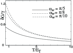
Figure 16: The $\delta G(T)$ dependence. Here $\gamma=\rho\xi_{h}/R_{b}$. $\Delta/E_{T}\gg 1$ and $w/L=0.05$ (from Bergeret, Volkov, and Efetov (2001a)).

In FIG. 16 we present the temperature dependence of the correction to the conductance  $\delta G(T).$ It is seen that with increasing the temperature $\delta G_{F}(T)$ decreases in a monotonous way. This dependence differs from the re-entrant behavior discussed above that occurs in the $S/N$ structures. The reason for this difference is that the time-reversal symmetry in $S/F$ structures is broken and this leads to a difference in transport properties. In a $S/N$ system, a relation$\hat{f}^{R}(\epsilon)=\hat{f}^{A}(\epsilon)|_{\epsilon=0}$ holds and this equality is a consequence the time-reversal symmetry. That is why $\delta G(0)=\delta G(T_{c})=0$ in $S/N$ structures, whereas in a $S/F$ structure $\hat{f}^{R}(\epsilon)\neq\hat{f}^{A}(\epsilon)|_{\epsilon=0}$ and that is why $\delta S(T)_{T=0}\neq 0.$

Although the LRTC may be the reason for the enhancement of the conductivity in the $S/F$ structures (this possibility was also pointed out in the work by Giroud et al. (2003)), our understanding is based on the assumption that the magnetic moment is fixed and does not change with the temperature. Dubonos et al. (2002) suggested another mechanism based on an assumption about a domain redistribution when the temperature drops below $T_{c}.$ The ferromagnetic wires (or strips) used in different experiments may consist of many domains. Their form and number depend on the sample geometry and parameters of the system. When the temperature decreases below $T_{c}$, stray magnetic fields excite the Meissner currents in the superconductor attached to the $F$ wire. Therefore the demagnetizing factors change, which may lead to a new domain structure. At the same time,  the total conductance (or resistance) $G_{F}$ depends on the form and the number of domains. So, one might expect that the conductance $G_{F}(T)$ below $T_{c}$ would differ from $G_{F}$ in the normal state. This idea was supported by measurements carried out by Dubonos et al. (2002). In this work a structure consisting of a two-dimensional electron gas and five Hall probes was used. An $F/S$ system ($Ni$+$Al$ disks) was placed on top of this structure. Measuring the Hall voltage, the authors were able to probe local magnetic fields around the ferromagnetic disks. They found that these fields really changed when the temperature dropped below $T_{c}$.

On the other hand, the Meissner currents and, hence, the effect of the redistribution of the domain walls may be considerably reduced in wires, as discussed previously. Changing the thickness of the superconducting wires in a controlled way and measuring the conductance could help to distinguish experimentally between the contribution to the conductivity of the triplet condensate and the effects of the redistribution of the domain walls.

An experiment in which the domain redistribution was excluded has been performed by Nugent et al. (2004). The authors measured the resistance variation of a ferromagnetic wire (Ni_1-xCu_x) lowering the temperature $T$ below the critical temperature $T_{c}$ of the superconductor (Al or Pb), which was attached to the middle part of the ferromagnetic wire. A magnetic field, strong enough to align all domains in the ferromagnet in one direction but not too strong to suppress the superconductivity, was applied to the system. Under these conditions a small increase in the resistance ($\delta R/R\approx 3\cdot 10^{-3}$) was observed when the temperature $T$ drops below $T_{c}$. The analysis presented above shows that the triplet component leads to an increase of the conductance but not in the resistance of the ferromagnetic wire. Therefore this particular experiment can hardly be explained in terms of the long-range proximity effect. Perhaps the small increase in the resistance of the ferromagnetic wire observed in Nugent et al. (2004) was related to the ”kinetic” mechanism discussed above (see Eq. (102)) or to weak localization corrections caused by the triplet Cooperons McCann et al. (2000). According to McCann et al. (2000) the change of the resistance of the ferromagnetic wire is positive (contrary to the contribution of the LRTC) and its order of magnitude is $(e^{2}/\hbar)R_{F}$, where $R_{F}$ is the resistance of the F wire in the normal state. In order to clarify the role of the LRTC in the transport properties of S/F structures, further theoretical and experimental investigations are needed. Note that strong ferromagnets like Fe are not suitable materials for observing the contribution of the LRTC into the conductance variation because of the strong exchange field $h$. In this case, according to Eq.(71) and Eq.(97), the amplitude of the LRTC is small because it contains $h$ in the denominator.

IV Josephson effect in S/F systems (inhomogeneous magnetization)

As we have mentioned above, one of the most interesting issues in the $S/F$ structures is the possibility of switching between the so called 0- and $\pi$-states in Josephson $S/F/S$ junctions. The $\pi$-state denotes the state for which the Josephson critical current $I_{c}$ becomes negative. This occurs for a certain thickness $d_{F}$ and temperature $T$. In this state the minimum of the Josephson coupling energy $E_{J}=(\hbar I_{c}/e)(1-\cos\phi)$ corresponds to a phase difference of $\phi=\pi$ but not to $\phi=0$ as in conventional Josephson junctions.

The reason for the sign reversal of $I_{c}$ is the oscillatory dependence of the condensate functions $\hat{f}$ on the thickness $d_{F}$ (see Eq.(37)). Since the critical current $I_{c}$ is sensitive to the phase of the condensate function at the boundary, the $\pi$-state is a rather natural consequence of the oscillations.

The possibility of the $\pi-$ state was predicted by Bulaevskii et al. (1977) and Buzdin et al. (1982), and studied later in many other works (e.g. Radovic et al., 1991; Buzdin and Vujicic, 1992). Experimentally, this phenomenon manifests in a non-monotonic dependence of the critical temperature on the thickness of the junction observed in many experiments and discussed in Section II.2.2. Another manifestation of the transition from the $0$- state to the $\pi$- state is the sign reversal of the critical current observed in the experiment by Ryazanov et al. (2001) on $Nb/Cu_{x}Ni_{1-x}/Nb$ Josephson junctions (see FIG. 5). The proper choice of an alloy with a weak ferromagnetic coupling was crucial for the observation of the effect.

Subsequent experiments, Kontos et al. (2002), Blum et al. (2002) and Guichard et al. (2003), corroborated the observed change of the sign of the Josephson coupling varying the thickness of the intermediate $F$ layer. Qualitatively, the experimental data on the Josephson effect in the $S/F/S$ structures are in agreement with the theoretical works above mentioned. However, a more accurate control and understanding of the $0$-$\pi$ transition demands knowledge of the magnetic structure of the ferromagnetic materials.

Almost in all theoretical papers very simplified models of the $S/F/S$ junction were analyzed. For example, Blanter and Hekking (2004) assumed that the $F$ layer consisted either of one domain or two domains with the collinear orientation of the magnetization. In this case and according to the discussion of section III.3 the LRTC is absent in the system.

If the $F$ layer is a single domain layer, the critical current $I_{c}$ is maximal at a non-zero external magnetic field $H_{ext}$ equal to $-4\pi M_{F}$, where $M_{F}$ is the magnetization of the $F$ layer. At the same time, in experiments Ryazanov et al. (2001); Kontos et al. (2001, 2002); Blum et al. (2002); Strunk et al. (1994); Sellier et al. (2004) a decrease of the current $I_{c}$ with increasing field $H_{ext}$ was observed and it was maximal at $H_{ext}=0$. This means, as it was assumed in these experimental works, that the F layer in real junctions contains many magnetic domains. In this case the Josephson critical current $I_{c}$ may change sign in the $S/F/S$ junctions with a multidomain magnetic structure even if the local Josephson current density $j_{c}$ is always positive. The reason for the sign reversal of $I_{c}$ in this case is a spatial modulation of the phase difference $\phi(x)$ due to an alternating magnetization $M\left(x\right)$ in the domains Volkov and Anishchanka (2004). In order to determine the mechanism that leads to the sign reversal of the critical current further experiments are needed.

In this chapter we discuss a new phenomenon, namely,  how the Josephson coupling between the $F$ layers in the $S/F$ structures is affected by the LRTC.

First, we consider a planar $S/F/S$ Josephson junction with a ferromagnet magnetization $\mathbf{M_{F}}$ rotating in the direction normal to the junction plane. This model is an idealization of a real multidomain structure with different magnetization orientations. In this case, as we discussed in Section III.4, the LRTC arising in the structure affects strongly the critical current $I_{c}.$

Next, we will analyze a multilayered $S/F/S/$… structure in which the vector $\mathbf{M}_{F}$ has a different direction in different $F$ layers. Again, in this case the LRTC arises in the system. Interestingly, if the thickness of the $F$ layers $d_{F}$ is much larger than the penetration length $\xi_{F}$ of the singlet component but less or of the order of $\xi_{N}$, then the Josephson coupling between the $F$ layers is realized due to the LRTC (odd triplet superconductivity in the transverse direction). At the same time, the  in-plane superconductivity is due to the conventional singlet superconducting pairing.

Finally we will discuss the dc Josephson effect in a $SF/I/FS$ junction (here $SF$ is a superconductor-ferromagnet bilayer and $I$ is a thin insulating layer). In this structure, the exchange field may lead not only to a suppression of the Josephson coupling as one could naively expect but, under a certain condition, to its enhancement.

Let us consider first a planar $S/F/S$ Josephson junction. We assume the following spacial dependence of the magnetization vector in the F layer: $\mathbf{M}_{F}=M_{F}(0,\sin(Qx),\cos(Qx))$, where the $x$-axis is normal to the junction plane.

In this case, as we have seen in Section III.3.2, the LRTC arises. Due to the long range penetration into the ferromagnet the triplet component can give a very important contribution to the Josephson current. A general expression for the Josephson current can be written in the form

$$I_{J}=(L_{y}L_{z}/4e)\sigma_{F}(\pi T)\mathrm{Tr(}\hat{\sigma}_{0}\otimes\hat{\tau}_{3}.\sum_{\omega}\check{f}_{\omega}\partial_{x}\check{f}_{\omega})\;.$$ (109)

We assume that the impurity concentration is sufficiently high and therefore the condensate function $\check{f}_{\omega}$ should be found from the Usadel equation. In the limit of a weak proximity effect (the $S/F$ interface transparency is not too high) this equation can be linearized and solved exactly. The solution for the $\check{f}_{\omega}$ matrix in the $F$ region can be found in a similar way as it was done in Section III.3.2. Due to the rotation of the magnetization the condensate function contains the LRTC. We obtain for the Josephson current Bergeret et al. (2001c) the following expression

$$I_{J}=I_{c}\sin\phi$$ (110)

where the critical current $I_{c}$ is equal to

$$I_{c}=(L_{y}L_{z}\sigma_{F}/l)\tilde{\gamma}_{F}^{2}\mathrm{Re}\sum_{\omega>0}f_{s}^{2}\left[\frac{e^{-\kappa_{+}d_{F}}}{\kappa_{+}l}+\frac{(Ql)^{2}e^{-\kappa_{l}d_{F}}}{2(3h\tau)^{3/2}}\right]\;,$$ (111)

and $\kappa_{l}^{2}=2|\omega_{n}|/\Delta+Q^{2}$. The parameter $\tilde{\gamma}_{F}=(3/4)<\mu T(\mu)>$ is an effective, averaged over angles, transmittance coefficient which characterizes the S/F interface transparency and $\kappa_{+}$ is defined in Eq. (89)

The first term in the brackets containing the parameter  $\kappa_{+}$corresponds to Eq. (36).  It decays by increasing the thickness $d_{F}$ over the short characteristic length $\xi_{F}=\sqrt{D_{F}/h}$ and can change the sign. The second term in Eq. (111)  originates from  the rotation of $h$ along the $x$-axis. It decays with the thickness $d_{F}$ over another characteristic length $\kappa_{l}^{-1}$ that can be much larger than $\xi_{F}$. Therefore this term results in a drastic change of the critical current.

The presence of the second term in Eq. (111) is especially interesting in the case when the thickness $d_{F}$ of the ferromagnetic spacer between the superconductors obeys $\xi_{F}<d_{F}<\kappa_{l}^{-1}$. Then the main contribution to the Josephson coupling comes from the long-range triplet component of the condensate. Another important feature of this limit is that for sufficiently large values of $Ql$ the critical current is always positive (no possibility for the $\pi$-contact). This can be seen from FIG. 7.

The fact that the superconductivity looses its “exotic properties” at large $Q$ is quite understandable. The superconductivity is sensitive not to the local values of the exchange field but to its average on the scales of the order of the superconducting coherence length. If the exchange field oscillates very fast such that the period of the oscillations is much smaller than the superconducting coherence length, its average on this scale vanishes and therefore all new properties of the superconductivity originating from the presence of the exchange field become negligible.

To conclude this introduction we summarize the results known for $S/F/S$ Josephson junctions.

When the magnetization in the ferromagnetic  $F$ is homogeneous, we have to distinguish between two different  cases.

In the dirty limit ($h\tau\ll 1$) the change of the sign of the critical current occurs if the thickness of the $F$ layer $d_{F}$ is of the order of $\xi_{F}$. The condensate function in the $F$ layer decays exponentially over this $\xi_{h}$ and oscillates with the same period.

In the opposite clean limit, $h\tau\gg 1$, the condensate function oscillates in space with the period $v_{F}/h$ and decays exponentially over the mean free path $l$.

Finally, if the ferromagnetic region contains a domain wall described by a vector $Q$, a long-range component of the condensate appears. It decays in the $F$ film over a considerably larger length of the order $\xi_{N}=\sqrt{D/2\pi T}$ that can greater exceed the characteristic length ($\sim\sqrt{D/h}$) in a homogeneous $F$ layer ($Q=0$). In this case the coupling between the superconductors survives even if the thickness of $F$ is larger than $\xi_{F}$.

It is clear that the presence of a domain wall between the superconductors is something that cannot be controlled very well experimentally. Therefore in the next section we discuss a possible experiment on $S/F$ multilayered structures that may help in detecting  the LRTC by measuring the Josephson critical current.

IV.1 Josephson coupling between S layers via the triplet component

In this subsection we analyze another type of multilayered $S/F$ structure in which the LRTC arises. This is a multilayered periodic $...S/F_{n-1}/S/F_{n}/S/F_{n+1}/S...$ structure with alternating magnetization vector $\mathbf{M}_{F,n}$ in different $F$ layers. We assume that the vector $\mathbf{M}_{F,n}$ is turned  with respect to the vector $\mathbf{M}_{F,n-1}$ by an angle $2\alpha$, such that the angle increases monotonously with increasing $n$. We call this arrangement of the magnetization the one with a positive chirality.

In an infinite system the magnetization vector $\mathbf{M}_{F}$ averaged over $n$ is equal to zero (it rotates when one moves from the $n-th$ to the ($n+1)-th,$ layer etc.). Another type of chirality (negative chirality) is the arrangement  when the angle between vectors $\mathbf{M}_{F,n}$ and $\mathbf{M}_{F,n-1}$ is equal to $2\alpha(-1)^{n}$. In this case the averaged vector $\mathbf{M}_{F}$ is not zero.

In Section III.3.1 we have seen that in a $F/S/F$ structure with a non-collinear orientation of the magnetization vectors in the $F$ layers the LRTC arises. If one assumes that the thickness of the $F$ layers $d_{F}$ is larger than the coherence length in the normal metal   $\xi_{N},$ the overlap of the condensate functions created in a $F$ layer by neighboring $S$ layers is weak, and the solutions given by Eqs.(58-66) remain valid for the multilayered $S/F$ structure.

Using these solutions one can calculate the Josephson current between neighboring $S$ layers. As the thickness $d_{F}$ is assumed to be much larger than $\xi_{F}$ (as usual, we assume that $\xi_{F}<<\xi_{N}$), the Josephson coupling between the $S$ layers is solely due to the LRTC. So, in such systems we come to a new type of the superconductivity: an odd triplet out-of-plane superconductivity and the conventional singlet in-plane superconductivity (the triplet component gives  only a small   contribution to the in-plane superconductivity).

Using the general Eqs. (58-66) one can perform explicit calculations for this case without considerable difficulties. As a result, the Josephson critical current $I_{c}$ can be written as follows Bergeret et al. (2003)

$$eR_{F}I_{c}=\pm 2\pi T\sum_{\omega}\kappa_{\omega}d_{F}b_{1}^{2}(\alpha)\left(1+\tan^{2}\alpha\right)e^{-d_{F}\kappa_{\omega}}\;,$$ (112)

where

$$b_{1}(\alpha)=-f_{BCS}\sin\alpha\frac{\mbox{$\tilde{\kappa}$}_{S}^{2}(\mbox{$\tilde{\kappa}$}_{+}-\mbox{$\tilde{\kappa}$}_{-})\mbox{${\rm sgn}$}\omega}{\cosh^{2}\Theta_{S}\left(M_{+}T_{-}+M_{-}T_{+}\right)(g_{BCS}+\gamma_{F}\kappa_{\omega}\tanh\Theta_{F})}\;,$$

$\Theta_{S}=\kappa_{s}d_{S}$, $\Theta_{F}=\kappa_{\omega}d_{F}$, $\mbox{$\tilde{\kappa}$}_{\pm}=\kappa_{\pm}/(g_{BCS}+\gamma_{F}\kappa_{\pm})$, $\mbox{$\tilde{\kappa}$}=\kappa_{\omega}/(g_{BCS}+\gamma_{F}\kappa_{\omega}\tanh\Theta_{F})$, $\mbox{$\tilde{\kappa}$}_{S}=\kappa_{S}/(g_{BCS}\gamma)$ and

$$M_{\pm} = T_{\pm}(\mbox{$\tilde{\kappa}$}_{S}\coth\Theta_{S}+\mbox{$\tilde{\kappa}$}\tanh\Theta_{F})+\tan^{2}\alpha\,C_{\pm}(\mbox{$\tilde{\kappa}$}_{S}\tanh\Theta_{S}+\mbox{$\tilde{\kappa}$}\tanh\Theta_{F})$$

$$T_{\pm} = \mbox{$\tilde{\kappa}$}_{S}\tanh\Theta_{S}+\mbox{$\tilde{\kappa}$}_{\pm}$$

$$C_{\pm} = \mbox{$\tilde{\kappa}$}_{S}\coth\Theta_{S}+\mbox{$\tilde{\kappa}$}_{\pm}\;.$$

$R_{F}$ is defined as $R_{F}=2d_{F}/(L_{y}L_{z}\sigma_{F})$. Eq. (112) describes the layered systems with both the positive (“+” sign) and negative (“-” sign) chirality.

One can see from Eq. (112) that in the case of positive chirality the critical current is positive, while if the chirality is negative the system is in the $\pi$-state (negative current). This means that changing the configuration of the magnetization, one can switch between the $0$ and $\pi$ state.

It is important to emphasize that the nature of the $\pi$-contact obtained here differs from that predicted by Bulaevskii et al. (1977) and observed by Ryazanov et al. (2001). In the latter cases the transition is due to the change of the values of either the exchange field, the temperature or the thickness of the $F$ film. In the case considered in this section, the negative Josephson coupling originates from the presence of the triplet component and can be realized in $S/F$ structures with negative chirality. Since for the positive chirality the Josephson current is positive, the result obtained gives an unique opportunity to switch experimentally between the $0$ and $\pi$-states by changing the angles of the mutual magnetization of the layers.

A similar dependence of the Josephson current $I_{c}$ on the chirality was predicted in a Josephson junction $S_{m}IS_{m}$ ($I$ is an insulator) between two magnetic superconductors $S_{m}$ by Kulic and Kulic (2001). For the magnetic superconductors considered in that work, the magnetization vector $\mathbf{M}$ rotated with the angle of rotation equal to $\alpha=x\mathbf{Q\cdot n}_{x}\mathbf{,}$where $\mathbf{Q}$ is the wave vector of the x- dependence of the angle $\alpha$, $\mathbf{n}_{x}$ is the unit vector normal to the insulating layer $I.$ Therefore the chirality (or spiral helicity, in terms of Kulic and Kulic) in this case is determined by the sign of the product $\mathbf{Q}_{R}\mathbf{\cdot Q}_{L},$ where $\mathbf{Q}_{L,R}$ is the wave vector in the left (right) magnetic superconductor.

However, there is an essential difference between the multilayered $S/F$ structure discussed here and the magnetic superconductors. In the magnetic superconductors with a spiral magnetization the triplet component also exists but, in contrast to the $S/F$ structures, the singlet and triplet components cannot be separated. In particular, in the case of a collinear alignment of $\mathbf{M,}$ the Josephson coupling in the $S/F$ structures with thick $F$ layers disappears, whereas it remains finite  in the $S_{m}IS_{m}$ system.

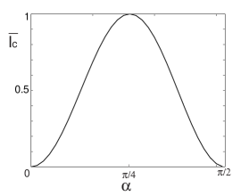
Figure 17: FIG. 16: Dependence of the critical current on the angle $\alpha$. The value of the current is given in arbitrary units (from Bergeret, Volkov, and Efetov (2003)).

FIG. 17 shows the dependence of the Josephson current $I_{c}$ on the angle $\alpha$ given by Eq. (112). If the mutual  orientation of $\mathbf{M}$ is parallel ($\alpha=0$) or antiparallel ($2\alpha=\pi$) the amplitude of the triplet component is zero and therefore there is no coupling between the neighboring $S$ layers, i.e. $I_{c}=0$. For any other angles between the magnetizations the amplitude of the triplet component is finite and this leads to a non-zero critical current. At $2\alpha=\pi/2$ ( perpendicular orientation of $\mathbf{M}$) the Josephson current $I_{c}$ reaches its maximum value.

Another possible experiment for detecting the long range triplet component is the measurement of the density of states in the $F/S/F$ system as it is shown in FIG. 18. Kontos et al. (2001) determined the spatial changes of the DOS in a $PdNi/Al$ structure with the help of planar tunnelling spectroscopy. This method could also  be used in order to detect the LRTC. It is clear that if the thickness of the $F$ layer in FIG. 18 is larger than the penetration of the short-range components, then any change of the DOS at the outer boundary of the $F$ layer may occur only due to the long range penetration of the  triplet component. If the magnetizations of both $F$ layer are collinear no effect is expected to  be observed, while for a non-collinear magnetization a change of the DOS should be seen.

Figure 18: Schematic: Measurement of the change of the density of states at the outer F interface by tunnelling spectroscopy. Kontos et al. (2001) performed such experiments on S/F structures.

IV.2 Enhancement of the critical Josephson current

Another interesting effect in the $S/F$ structures that we would like to discuss is the enhancement of the Josephson critical current by the exchange field. The common wisdom is that any exchange field should reduce or destroy the singlet superconductivity. In the previous sections we have seen that this is not always so and the superconductivity can survive in the presence of a strong exchange field. But still, it is not so simple to imagine that the superconducting properties can be enhanced by the exchange field.

Surprisingly, this possibility exists and we will demonstrate now how this unusual phenomenon occurs. Although the LRTC is not essential to get the critical current enhancement, the short-range triplet component arises in this case and it plays a certain role in this effect. The enhancement of the Josephson current in the $S/F/I/F/S$ tunnel structures ($I$ stands for an insulating layer, see FIG. 19) was predicted by Bergeret et al. (2001b) and further considered in a subsequent work by Golubov et al. (2002b). As we will see below, if the temperature is low enough and the $S/F$ interface transparency is good, one can expect an enhancement of the critical current with increasing the exchange field provided the magnetizations of the $F$ layers are antiparallel to each other.

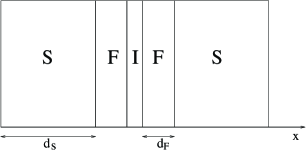
Figure 19: The S/F/I/F/S system. I is an insulating thin layer.The relative magnetization of the F layers can be switched.

This surprising result can be obtained in a quite simple way in the limit when  the thicknesses $d_{S}$ and $d_{F}$ of the $S$ and $F$ layers are smaller than the superconducting coherence length $\xi_{S}\sim\sqrt{D/2\pi T_{c}}$ and the penetration length of the condensate into the ferromagnet $\xi_{F}\sim\sqrt{D/h}$, respectively. In this case one can assume that the quasiclassical Green’s functions does not depend on the space coordinates and, in particular, the superconducting order parameter $\Delta$ is a constant in space. Moreover, instead of considering the dependence of the exchange field $h$ on the coordinates one can replace it by a homogeneous effective exchange field $h_{eff}$ with a reduced value. Therefore we use in our calculations effective fields $\Delta_{eff}$ and $h_{eff}$ defined as

$$\Delta_{eff}/\Delta = \nu_{S}d_{S}\left(\nu_{S}d_{S}+\nu_{F}d_{F}\right)^{-1}\;,$$ (113)

$$h_{eff}/h = \nu_{F}d_{F}\left(\nu_{S}d_{S}+\nu_{F}d_{F}\right)^{-1}\;,$$ (114)

where $\nu_{S}$ and $\nu_{F}$ are the densities of states in the superconductor and ferromagnet, respectively.

With this simplification,  we can write the Gor’kov equations for the normal and anomalous Green’s functions in the spin-space as

$$\left(i\omega+\xi-\mathbf{\sigma h}\right)\hat{G}_{\omega}+\hat{\Delta}\hat{F}_{\omega}^{+} = 1$$ (115)

$$\left(-i\omega+\xi-\mathbf{\sigma h}\right)\hat{F}_{\omega}+\hat{\Delta}\hat{G}_{\omega} = 0\;,$$ (116)

where $\mathbf{\sigma}=(\mbox{$\hat{\sigma}_{1}$},\mbox{$\hat{\sigma}_{2}$},\mbox{$\hat{\sigma}_{3}$})$ are the Pauli matrices and $\xi=\epsilon\left(\mathbf{p}\right)-\epsilon_{F},$ $\varepsilon_{F}$ is the Fermi energy, $\varepsilon\left(\mathbf{p}\right)$ is the spectrum, and $\omega=\left(2n+1\right)\pi T$ are Matsubara frequencies. (We omit the subscript $eff$  in Eqs. (115-116) and below).

In order to calculate the Josephson current $I_{J}$ through the tunnel junction represented in FIG. 19 we use the well known standard formula

$$I_{J}=\left(2\pi T/eR\right)\mathrm{Tr}\sum_{n}\hat{f}_{\omega}(h_{1})\hat{f}_{\omega}(h_{2})\sin\varphi\;,$$ (117)

where

$$\hat{f}_{\omega}=\frac{i}{\pi}\int{\hat{F}_{\omega}\mathrm{d}\xi}$$ (118)

is the quasiclassical anomalous Green’s function, $\varphi$ is the phase difference between both the superconductors, $R$ is the barrier resistance and $h_{1,2}$ are the exchange fields of the left and the right $F$-layers.

The only difference between Eqs. (117, 118) and the corresponding equations in the absence of the exchange field is the dependence of the condensate function $\hat{f}_{\omega}$ on $h$. This dependence can be found immediately from Eqs. (115, 116).

$$\hat{f}_{\omega}=\hat{\Delta}\left(\left(\omega+i\mathbf{\sigma h}\right)^{2}+\Delta^{2}\right)^{-1/2}$$ (119)

What remains to be done is to insert the condensate function $\hat{f}$ into Eq. (117) for certain exchange fields $h_{1}$ and $h_{2}$ and to calculate the sum over the Matsubara frequencies $\omega$. Although it is possible to carry out these calculations for arbitrary vectors $h_{1}$ and $h_{2},$ we restrict our consideration by the cases when the absolute values the magnetizations $h_{1}$ and $h_{2}$ are equal but the magnetizations are either parallel or antiparallel to each other. This simplifies the computation of the Josephson current but, at the same time, captures the essential physics of the phenomenon.

Using Eqs. (117-119) and assuming first that $h_{1}$ and $h_{2}$ are parallel to each other we write the expression for the critical current as Bergeret et al. (2001b)

$$I_{J}=I_{c}\sin\varphi$$ (120)

$$I_{c}^{\left(p\right)}\!\!=\frac{\Delta^{2}\left(T\right)4\pi T}{eR}\sum_{\omega}\frac{\omega^{2}+\Delta^{2}\left(T,h\right)-h^{2}}{\left(\omega^{2}+\Delta^{2}\left(T,h\right)-h^{2}\right)^{2}+4\omega^{2}h^{2}},$$ (121)

The corresponding equation for the antiparallel configuration is different from Eq. (121) and can be written as

$$I_{c}^{\left(a\right)}\!\!=\frac{\Delta^{2}\left(T\right)4\pi T}{eR}\sum_{\omega}\frac{1}{\sqrt{\left(\omega^{2}+\Delta^{2}\left(T,h\right)-h^{2}\right)^{2}+4\omega^{2}h^{2}}}.$$ (122)

One can easily check that the critical current $I_{c}^{\left(p\right)}$ for the parallel configuration, Eq. (121), is always smaller than the current $I_{c}^{\left(a\right)}$ for the antiparallel case. These two expressions are equal to each other only in the absence of any magnetization.

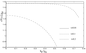
Figure 20: Dependence of the normalized critical current on $h$ for different temperatures in the case of a parallel orientation. Here $eV_{c}=eRI_{c}$, $h_{F}$ is the effective exchange field, $t=T/\Delta_{0}$ and $\Delta_{0}$ is the superconducting order parameter at $T=0$ and $h=0$

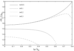
Figure 21: The same dependence as in FIG. 20 in the case of an antiparallel orientation.

In FIGS. 20 and 21 we represent the dependence of the critical current on the strength of the exchange field.  We see from FIG. 20 that for the parallel configuration the exchange field reduces the value of the Josephson current and this is exactly what one could expect. At the same time, the critical current grows with the exchange field for the antiparallel configuration at low temperatures, which is a new intriguing effect (see FIG. 21).

This unexpected result can be understood from Eq. (122) rather easily without making numerics. In the limit $T\rightarrow 0$ the sum over the  Matsubara frequencies can be replaced by an integral and one can take for the superconducting order parameter $\Delta$ the values $\Delta=\Delta_{0}$ if $h<\Delta_{0},$ and $\Delta=0$ if $h>\Delta_{0}$, where $\Delta_{0}$ is the BCS order parameter in the absence of an exchange field (see, e.g. Larkin and Ovchinikov (1964)).

Inserting this solution into Eq. (122) one can see that the Josephson critical current $I_{c}^{\left(a\right)}$ grows with increasing exchange field. Moreover, formally it diverges logarithmical when $h\rightarrow\Delta_{0}$

$$I_{c}^{\left(a\right)}\left(h\rightarrow\Delta_{0}\right)\simeq\frac{I_{c}\left(0\right)}{\pi}\ln\left(\Delta_{0}/\omega_{0}\right)\,,$$ (123)

where $I_{c}\left(0\right)$ is the critical current in the absence of the magnetic moment at $T=0$, and $\omega_{0}$ is a parameter needed to cut the logarithm at low energies.

When deriving Eqs. (121, 122) the conventional singlet superconducting pairing was assumed. The electrons of a Cooper pair have the opposite spins. This picture of a superconducting pairs with the opposite spins of the electrons helps in the understanding of the effect.

If the magnetic moments in both the magnetic layers are parallel to each other, they serve as an obstacle for the Cooper pair because the pairs located in the region of the ferromagnet demand more energy. This leads to a reduction of the Josephson current. However, if the exchange fields of the different layers are antiparallel, they may favor the location of the Cooper pairs in the vicinity of the Josephson junction. A certain probability exists that one of the electrons of the pair is located in one layer, whereas the other is in the second layer. Such a possibility is energetically favorable because the spins of the electrons of the pair can now have the same direction as the exchange fields of the layers. Then it is more probable for the pairs to be near the junction even in comparison with a junction without exchange fields and, as a result, the critical current may increase.

The results presented above have been obtained for the $SF/I/FS$ structure by Bergeret et al. (2001b). Earlier a formula for the Josephson critical current in the $S_{m}IS_{m}$ ($S_{m}$  is the magnetic superconductor) junction was presented by Kulic and Kulic (2001). From that formulae one could, in principle, derive an enhancement of the critical current for the antiparallel $M$ orientation in magnetic superconductors $S_{m}$. Unfortunately, the authors seem to have missed this interesting effect.

Some remarks should be made at this point:

1) The results presented above are valid in the tunnelling regime, i.e. when the transparency of the insulating barrier $I$ is low enough. Golubov et al. (2002b) have shown that a smearing of the singularity of $I_{c}^{(a)}$ is provided by a finite temperature or a not very low barrier transparency. The maximum of the critical current for the antiparallel configuration $I_{c}^{(a)}$ decreases with decreasing resistance of the $I$ layer. The effect becomes weaker as the thickness of the $F$ layer grows.

2) We assumed that the $S/F$ interface was perfect. In a structure with a large $S/F$ interface resistance $R_{S/F}$ the bulk properties of the $S$ film are not considerably influenced by the proximity of the $F$ film (to be more precise, the condition $R_{S/F}>(\nu_{F}d_{F}/\nu_{S}d_{S})\rho_{F}\xi_{F}$ must be satisfied, where $\rho_{F}$ is the specific resistance of the $F$ film). Then, as one can readily show (see section II.2), a minigap $\epsilon_{bF}=\left(D\rho\right)_{F}/\left(2R_{S/F}d_{F}\right)$ arises in the $F$ layer. The Green’s functions in the $F$ layers have the same form as before with $\Delta$ replaced by $\epsilon_{bF}$. The singularity in $I_{c}(h)$ first occurs at $h$ equal to $\epsilon_{bF}$.

A physical explanation for the singular behavior of the critical current $I_{c}^{(a)}$ was given by Golubov et al. (2002b) These authors noticed that the density of states in the $F$ layer has a singularity when $h=\epsilon_{bF}$. At this value of $h$ the maximum of $I_{c}^{(a)}$ is achieved due to an overlap of two $\epsilon^{-1/2}$ singularities. This leads to the logarithmic divergency of the critical current in the limit $T\rightarrow 0$ in analogy with the well known Riedel peak in $SIS$ tunnel junctions for the voltage difference $2\Delta$. In the latter case the shift of the energy is due to the electric potential.

Golubov et al. (2002b) have also  shown that for the parallel configuration, at $h=\epsilon_{bF}$ the critical current changes its signs, i.e. there is a transition from $0$ to a $\pi$ junction. Similar results were obtained by Krivoruchko and Koshina (2001a, b). The case of an arbitrary $S/F$ transparency was also studied by Li et al. (2002); Chtchelkatchev et al. (2002); Barash et al. (2002). In the paper by Barash et al. (2002) the authors calculated the Josephson current as a function of the angle between the magnetizations in the $F$ film.

V Reduction of the Magnetization due to Superconductivity: Inverse Proximity Effect

Until now we have been studying the superconducting properties of different $S/F$ structures for a fixed magnetization. This means that we assumed a certain value for this quantity and its dependence on coordinates. The implied justification of this assumption was that the ferromagnetism is a stronger phenomenon than the superconductivity and the magnetic moment of conventional ferromagnets can hardly be affected by the superconductivity.

This assumption is certainly correct in many cases but not always. Often the presence of the superconductivity can drastically change magnetic properties of the ferromagnets even if they are strong.

Experiments performed by Mühge et al. (1998) and Garifullin et al. (2002) showed that the total magnetization of certain $S/F$ bilayers with strong ferromagnets decreased with lowering the temperature below the critical superconducting transition temperature $T_{c}$. As an explanation, it was suggested that due to the proximity effect domains with different magnetization appeared in the magnetic materials and this could reduce the total magnetization. At the same time, quantitative estimates based on an existing theory Buzdin and Bulaevskii (1988) led to a conclusion that this mechanism was not very probable.

In this Chapter we address the problem of the reduction of the magnetic moment by the presence of a superconductor assuming again that, in the absence of the ferromagnet, we would have the conventional singlet superconducting pairing. It turns out that two different and independent mechanisms that lead to a decrease of the magnetization in $S/F$ heterostructures due to the proximity effect exist and we give a detailed account of them.

In order to study the magnetic properties we have to choose a model. One can distinguish two different types of the ferromagnetism: a) itinerant ferromagnetism due to the spin ordering of free electrons and b) ferromagnetism caused by localized spins. Most of ferromagnetic metals show both of the types of ferromagnetism simultaneously, i.e. their magnetization consists of both contributions.

We consider a model in which the conducting electrons interact with the localized moments via an effective exchange interaction. The corresponding term in the Hamiltonian is taken in  the form (see Appendix A):

$$-\int d^{3}r\psi^{\dagger}(\mathbf{r})_{\alpha}\left(J\mathbf{S(r)}\mathbf{\sigma})\right)_{\alpha\beta}\psi(\mathbf{r})_{\beta}\;.$$ (124)

This term is suitable to describe $s-d$ or $s-f$ interaction between the $s$ and localized $d$ and $f$ electrons. We also consider the ferromagnetic interaction between the localized moments. This interaction can be very complicated and to determine it, one should know the detailed band structure of the metal as well as different parameters.  However, all these details are not important for us and we write the interaction between the localized spins  phenomenologically as

$$-\sum_{ij}\mathcal{J}_{ij}\mathbf{S}_{i}\mathbf{S}_{j}\;.$$ (125)

It is assumed that $\mathcal{J}$ is positive. This interaction, Eq. (125) , is responsible for the ferromagnetic alignment of the localized moments and is known as the Heisenberg Hamiltonian.

So , we consider a metallic ferromagnet in which the conduction electrons interact with localized magnetic moments. The ferromagnetic interaction (125) assures a finite magnetic moment of the background. The total magnetization is the sum of the background magnetization (localized moments) and the magnetization of the polarized free electrons.

In the next two sections we discuss the  two different mechanisms that lead to a decrease of the magnetization at low temperatures. In Section V.1 we consider a possibility of changing the magnetic order of the localized magnetic spins in a $F$ film deposited on top of a bulk superconductor. The contribution from free electrons to the magnetization is first assumed to be small. We will see that for not too strong ferromagnetic coupling $\mathcal{J}$ the proximity effect may lead to an inhomogeneous magnetic state. Contrary to this case, we consider in Section V.2 an itinerant ferromagnet in which the main contribution to the magnetization is due to free electrons. We will show that the magnetization of free electrons may decrease at low temperatures  due to a some kind of spin screening. Thus, both effects may lead to the decrease in the magnetization observed in experiments Mühge et al. (1998); Garifullin et al. (2002).

V.1 Cryptoferromagnetic state

In 1959 Anderson and Suhl suggested that superconductivity could coexist with a nonhomogeneous magnetic order in some type of materials. Anderson and Suhl called this state cryptoferromagnetic state.

The reason for this coexistence is that, if the magnetization direction varies over a scale smaller than the superconducting coherence length, the superconductivity may survive despite the ferromagnetic background. This is due to the fact that the superconductivity is sensitive to the ferromagnetic moment averaged on the scale of the size of Cooper pairs rather than to its local values.

In 1988 Buzdin and Bulaevskii discussed properties of a bilayer system consisting of a conventional superconductor in contact with a ferromagnet. They have shown that the magnetic ordering in the magnet might take the form of a structure consisting of small size domains, such that the superconductivity is not destroyed. Of course, as follows from Eq. (125), the formation of a domain-like structure costs a magnetic energy but this is compensated by the energy of the superconductor that would have been lost if the magnetic order remained ferromagnetic.

This is only possible if the stiffness of the magnetic order parameter ($\mathcal{J}$) is not too large. For instance this nonhomogeneous magnetization occurs in magnetic superconductors as those studied by Bulaevskii et al. (1985). But can one see it in the heterostructures containing strong ferromagnets like $Fe$ or $Ni$ in contact with conventional superconductors?

At first glance, it seems impossible, since the Curie temperature of, for example, iron is hundred times or more larger than the critical temperature of a conventional superconductor. Therefore any change of the ferromagnetic order look much less favorable energetically than the destruction of the superconductivity in the vicinity of the $S/F$ interface.

This simple argument was however questioned in the experiments performed by Mühge et al. (1998) on $Fe/Nb$ bilayers and by Garifullin et al. (2002) on $V/Pd_{1-x}Fe_{x}$ structures. Direct measurements of the ferromagnetic resonance has shown that in several samples with thin ferromagnetic layers the average magnetic moment started to decrease below the superconducting transition temperature $T_{c}$.

Of course, one can reduce the influence of the ferromagnet on the superconductor by diminishing the thickness of the ferromagnet. Using the formulae obtained by Buzdin and Bulaevskii (1988), Mühge et al. (1998) estimated the thickness of the ferromagnet for which the superconductivity was still possible and got a value of the order of $1$Å, which created a doubt on the explanation of the experiment in this way.

At the same time, the use of the formulae derived by Buzdin and Bulaevskii was not really justified because the calculations were done for thick but weak ferromagnets assuming a strong anisotropy of the ferromagnet that was necessary for a formation of the domain walls with the magnetization vector changing its sign but not its axis.

Bergeret, Efetov, and Larkin (2000) investigated theoretically the possibility of a cryptoferromagnetic-like (CF) state in $S/F$ bilayers with parameters corresponding to the experiments by Mühge et al. and Garifullin et al.. In that work a CF state with a magnetic moment that rotates in space was considered. This corresponds to a weak anisotropy of the ferromagnet, which was the case in the samples studied in Mühge et al. (1998). In particular, Bergeret et al. (2000) studied a phase transition between the CF and the ferromagnetic (FM) phases. The calculations were carried out in the limit $d_{F}\ll\xi_{h}=v_{0}/h,$ $T_{c}\ll h\ll\epsilon_{0}$, $v_{0}$ and $\epsilon_{0}$ are the Fermi velocity and Fermi energy, respectively. This limit is consistent with the parameters of the experiment of Mühge et al. (1998), Garifullin et al. (2002). We present here the main ideas of this work.

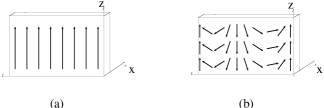
Figure 22: A S/F bilayer consisting of a thin ferromagnet attached to a bulk superconductor. The ferromagnet may be either in the (a) ferromagnetic or the (b) cryptoferromagnetic phase.

The Hamiltonian describing the bilayer structure in FIG. 22 can be written as

$$H\left(\gamma\right)=H_{0}+H_{BCS}-\gamma\int d\mathbf{r}\Psi_{\alpha}^{+}(\mathbf{r})\left[\mathbf{h}(\mathbf{r})\mathbf{\sigma}\right]_{\alpha\beta}\Psi_{\beta}(\mathbf{r})+H_{M}\;,$$ (126)

where the integration must be taken in the region $-d<x<0$. Here $H_{0}$ is the one-particle electron energy (including an interaction with impurities), $H_{BCS}$ is the usual term describing the conventional BCS superconductivity in the superconductor $S$ and the third term describes the interaction between localized moments and conduction electrons, where $\gamma$ is a constant that will be put to $1$ at the end (see Appendix A).

The term $H_{M}$ describes the interaction between the localized moments in the ferromagnet (cf. Eq.(125)). We assume that the magnetization of the localized spins is described by classical vectors and take into account the interaction between neighboring spins only. In the limit of slow variations of the magnetic moment in space with account of Eq. (125), the Hamiltonian $H_{M}$ can be written in the form

$$H_{M}=\int\mathcal{J}\left[\left(\mathbf{\nabla}S_{x}\right)^{2}+\left(\mathbf{\nabla}S_{y}\right)^{2}+\left(\mathbf{\nabla}S_{z}\right)^{2}\right]dV,$$ (127)

where the magnetic stiffness $\mathcal{J}$ characterizes the strength of the coupling between the localized moments in the $F$ layer and the $S_{i}$ are the components of a unit vector that are parallel to the local direction of the magnetization.

We assume that the magnetic moments are directed parallel to the $S/F$ interface and write the spin vector $\mathbf{S}$ as $\mathbf{S}=\left(0,-\sin\theta,\cos\theta\right)$. A perpendicular component of the magnetization would induce strong Meissner currents in the superconductor, which would require a greater additional energy.

The condition for an extremum of the energy $H_{M}$, Eq. (127) can be written as

$$\Delta\theta=0$$ (128)

Solutions of Eq. (128) can be written in the form $\theta=Qy$, where $Q$ is the wave vector characterizing the rotation in space (see FIG. 22). The value $Q=0$ corresponds to the ferromagnetic state.

What we want to do now is to compare the energies of the ferromagnetic and cryptoferromagnetic states. The latter will be considered for the case with a rotating in space magnetic moment $\theta=Qy$. This should be energetically more favorable than the domain-like structure one provided the magnetic anisotropy of $F$ is low. Such a CF state corresponds to a so called Neel wall (see for example Aharoni (1996)).

Strictly speaking, one has to take into account also a magnetostatic energy due to a purely magnetic interaction of the magnetic moments. However, if the condition

$$\frac{\mathcal{J}}{M_{s}^{2}}\gg d^{2}$$ (129)

where $M_{s}$ is the magnetic moment per volume, is fulfilled one can neglect its contribution with respect to the one of the exchange energy Aharoni (1996).

Taking typical values of the parameters for $Fe$: $M_{s}=800$emu/cm³ and $J=2.10^{-6}$erg/cm one can see that the condition (129) requires that the thickness $d$ of the ferromagnet is smaller than $10nm$, which corresponds to comparatively thick layers. Throughout this section this condition is assumed to be fulfilled.

In this case the magnetic energy $\Omega_{M}$ (per unit surface area) is given by the simple expression

$$\Omega_{M}=JdQ^{2}\;.$$ (130)

In order to calculate the superconducting energy $\Omega_{S}$ one has to take into account the fact that the order parameter should be destroyed, at least partially, near the contact with the ferromagnet. This means that the order parameter $\Delta$ is a function of the coordinate $x$ perpendicular to the interface. As we want to minimize the energy we should look for a non-homogeneous solution for $\Delta\left(x\right)$ of non-linear equations describing the superconductivity. Near the critical temperature $T_{c}$ one can use Ginzburg-Landau equations. The proper solution of these equations can be written in the form

$$\Delta\left(x\right)=\Delta_{0}\tanh\left(\frac{x}{\sqrt{2}\xi_{GL}\left(T\right)}+C\right)$$ (131)

where $\Delta_{0}$ the value of the order parameter in the bulk, and $\xi_{GL}$ is the correlation length of the superconductor defined in Eq. (2). Near $T_{c}$ this length can be much larger than the length $\xi_{S}$. The parameter $C$ in Eq. (131) is a number that has to be found from boundary conditions.

The solution for $\Delta\left(x\right)$, Eq. (131) is applicable at distances exceeding the length $\xi_{S}$ and therefore we cannot use it near the interface.

Having fixed the constant $C$ one can compute the decrease of the superconducting energy due to the suppression of superconductivity in the $S$ layer using the Ginzburg-Landau free energy functional (e.g. de Gennes, 1966). The decrease of the superconducting energy $\Omega_{S}$ per unit area at the $F/S$ interface is a function of $C$ and can be written as

$$\Omega_{S}=\frac{\sqrt{\pi}}{6\sqrt{2}}|\tau|^{3/2}\left(2+K\right)(1-K)^{2}\;,$$ (132)

where $K=\tanh C$, and $\tau=(T-T_{c})/T_{c}.$

It remains only to determine the contribution from the third term of the Hamiltonian (126). The corresponding free energy $\Omega_{M/S}$ is given by the expression:

$$\Omega_{M/S}=-i\pi T\nu_{0}\frac{\mathrm{Tr}}{2}\sum_{\omega}\int_{0}^{1}d\gamma\int d^{3}\mathbf{r}(\mathbf{h\sigma})\left\langle\hat{g}\right\rangle_{0}\;,$$ (133)

where $\nu_{0}$ is the density of states and $\left\langle\hat{g}\right\rangle_{0}$ is the quasiclassical Green’s function averaged over all directions of the Fermi velocity.

Since the exchange field $h$ in a strong ferromagnet may be much higher than the value of  $\tau^{-1}$ (here $\tau$ is the momentum relaxation time), one has to solve the Eilenberger equation in the $F$ region and the Usadel equation in the $S$ region. Solutions for these equations in both the superconductor and ferromagnet were obtained by Bergeret et al. (2000).

Thus, the total energy is given by $\Omega=\Omega_{M}+\Omega_{S}+\Omega_{M/S}$, Eqs. (130, 132, 133). As a result, one can express the free energy as a function of two unknown parameters, $K$ and $Q$. One can find these parameters from the condition that the free energy must be minimal, which leads to the equations

$$\partial{\ \Omega}/\partial K=\partial{\Omega}/\partial Q=0$$ (134)

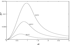
Figure 23: Phase diagrams ($\lambda,a$) for different values of $|\tau|=\frac{T_{c}-T}{T_{c}}$. The area above (below) the curves corresponds to the F (CF) state.

One can show that the CF-F transition is of second order, which means that near the transition the parameter $Q$ is small. At the transition it vanishes and this gives an equation binding the parameters. Solving the equation numerically we come to the phase diagram of FIG. 23 determining the boundary between the ferromagnetic and cryptoferromagnetic states. The parameters $a$ and $\lambda$ used in FIG. 23 are defined as

$$a^{2}\equiv\frac{2h^{2}d_{f}^{2}}{DT_{c}\eta^{2}},\;\;\;\lambda\equiv\frac{\mathcal{J}d_{F}}{\nu_{F}\sqrt{2T_{c}D^{3}}}\frac{7\zeta(3)}{2\pi^{2}},$$ (135)

where $\eta$ is the ratio between the Fermi velocities $v_{0}^{F}/v_{0}^{S}$. It is clear from Eqs.  (135) that the parameter $a$ is related to the exchange energy $h$, while $\lambda$ is the related to the magnetic stiffness $\mathcal{J}$.

The conclusion that the phase transition between F and CF states should be of the second order was drawn neglecting the magnetostatic interaction. The direct magnetic interaction can change this transition to a first order one Buzdin (2005b). However, in the limit of Eq. (129), this first order transition will be inevitably close to the second order one. Such a modification of the type of the phase transition is out of the focus of this review.

Let us make estimates for the materials used in the experiments. Performing ferromagnetic resonance measurements, Mühge et al. (1998) have observed a decrease of the effective magnetization of a $Nb/Fe$ bilayer. The stiffness $\mathcal{J}$ for materials like $Fe$ and $Ni$ is $\approx 60K/$Å. The parameters characterizing $Nb$ can be estimated as follows: $T_{c}\!=\!10K$ , $v_{F}\!\cong\!10^{8}$cm/s, and $l\!\cong\!100$Å. The thickness of the magnetic layer is of order $d\!=\!10$Å, and the exchange field $h\!\cong\!10^{4}K$ which is proper for iron.

Assuming that the Fermi velocities and energies of the ferromagnet and superconductor are close to each other, we obtain $a\approx 25$ and $\lambda\sim 6.10^{-3}$. It is clear from FIG. 23 that the cryptoferromagnetic state is hardly possible in the $Fe/Nb$ samples used in the experiment Mühge et al. (1998).

However, one can in principle explain the observed, decrease of the magnetization taking a closer look at the structure of the $S/F$ interface. In the samples analyzed by Mühge et al. the interface between the $Nb$ and $Fe$ layers is rather rough. So, one can expect that in the magnetic layers there were “islands” with smaller values of $\mathcal{J}$ and/or $h$. A reduction of these parameters in the $Fe/Nb$ bilayers is not unrealistic because of the formation of non-magnetic “dead” layers that can also affect the parameters of the ferromagnetic layers. If the cryptoferromagnetic state were realized only on the islands, the average magnetic moment would be reduced but would remain finite. Such a conclusion correlates with what one observes experimentally. One can also imagine islands very weakly connected to the rest of the layer, which would lead to smaller energies of a non-homogeneous state.

Let us now consider the experiment by Garifullin et al. (2002) on $Pd_{0.97}Fe_{0.03}/V$. Due to the low concentration of iron, the magnetic stiffness and the exchange field of the $F$-layers is much lower than the one in the case of a pure iron. For this system, one estimates the parameters as(see Garifullin et al. (2002)) $J\sim 60K/nm$, $h\sim 100K$. Assuming again that the Fermi velocities of $V$ and $Pd_{1-x}Fe_{x}$ are close to each other, Garifullin et al. (2002) obtained for the sample with $d_{F}=1.2$nm the following values of the parameters $a\sim 1.2$ and $\lambda\sim 1.3.10^{-3}$.

Using these values for $a$ and $\lambda$ one can see from the phase diagram in FIG. 23 that  there can be a transition from the F to the CF state at $|\tau|\sim 0.2$, which corresponds to $T\sim 2.4K$. The decrease of the effective magnetization $M_{eff}$ with decreasing temperature was not observed in samples with larger $F$ thickness $d_{F}$: $M_{eff}$ was a temperature-independent constant for the sample with $d_{F}=4.4nm$ and $d_{S}=37.2nm$. In the sample with $d_{F}=1.2nm$ and $d_{S}=40nm$ the effective magnetization $M_{eff}$ decreased by $\approx 50\%$ with cooling from $T\approx 4K$ to $T\approx 1.5K$. This fact is again in accordance with the predictions of Bergeret et al. (2000).

The results of this section demonstrate that not only ferromagnets change superconducting properties but also superconductivity can affect ferromagnetism. This result is valid, in particular, for strong ferromagnets, although the thickness of the ferromagnetic layers must be small in this case.

The exchange interaction between the superconducting condensate and the magnetic order parameter reduces the energy of the system if the direction of the magnetization vector $M_{F}$ is not constant in space but oscillates. Provided the energy of the anisotropy is small, this interaction leads to the formation of a spiral magnetic structure in the $F$ film.

As we will see in the next section the appearance of the CF-state is not the only effect that leads to a reduction of the effective magnetization in S/F structures. We will show that the proximity effect may also lead to a change of the absolute value of the magnetic moment $M_{F}$ in the ferromagnet and to an induced magnetization $M_{S}$ in the superconductor.

V.2 Ferromagnetism induced in a superconductor

In the previous section we have seen that the superconductivity can affect the magnetic ordering changing the orientation of magnetic moments in the ferromagnetic film. In this section we want to demonstrate that another mechanism for a change of the total magnetization of a $S/F$ system exists. In contrast to the phenomenon discussed in the previous Section, the orientation of the magnetic moments in the $F$ film does not change but the magnitude of the magnetization both in the $F$ and $S$ films does.

This change is related to the contribution of free electrons both in the ferromagnet ($\delta M_{F}$) and in the superconductor ($M_{S}$) to the total magnetization. On one hand, the DOS in the $F$ film is reduced due to the proximity effect and therefore $\delta M_{F}$ is reduced. On the other hand, the Cooper pairs in the $S$ film are polarized in the direction opposite to $M_{F}$, where $M_{F}$ is the magnetization of free electrons in the ferromagnet.

Let us consider first a bulk ferromagnet and derive a relation between the exchange field and the magnetization of the free electrons. The exchange field $h=JS$ in the ferromagnet can be due to the  localized moments (see Eq. (124)) or due to the free electrons in the case of an itinerant ferromagnet In some ferromagnets both the  localized and itinerant moments contribute to the magnetization.

The magnetization of the free electrons is given by

$$M=\frac{i}{4}\mu_{B}\int\frac{d\omega}{2\pi}\int\frac{d^{3}p}{(2\pi)^{3}}\mathrm{Tr}\mbox{$\hat{\tau}_{3}$}\mbox{$\hat{\sigma}_{3}$}\left(\check{G}^{R}-\check{G}^{A}\right)n_{p}\;,$$ (136)

where $\mu_{B}$ is an effective Bohr magneton and $n_{P}$ is the Fermi distribution function of the free electrons. The expression in front of $n_{P}$ in Eq. (136) determines the DOS that depends on the exchange field $\mathbf{h}$. We assume that the magnetization is oriented along the $z$-axis.

Using Eq. (136) one can easily compute the contribution of the free electrons to the magnetization in a bulk ferromagnet. In the simplest case of a normal metal with a quadratic energy spectrum we have

$$M_{F}=\frac{\mu_{B}}{(2\pi)^{2}}\int p^{2}dp\left[n(\xi_{p}-h)-n(\xi_{p}+h)\right]\;,$$ (137)

where $\xi_{p}=p^{2}/2m-\epsilon_{F}$. At $T=0$ the  magnetization is given by:

$$M_{F0}=\frac{\mu_{B}}{2(3\pi^{2})}\left(p_{+}^{3}-p_{-}^{3}\right)\;$$ (138)

where $p_{\pm}=\sqrt{2m(\epsilon_{F}\pm h)}$ are the Fermi momenta for spin up and spin down electrons. In the quasiclassical limit it is assumed that $h\ll\epsilon_{F}$, and therefore

$$M_{F0}\cong\mu_{B}\nu h\,,$$ (139)

where $\nu=p_{F0}m/\pi^{2}$ is the density of states at the Fermi level, and $p_{F0}=\sqrt{2m\epsilon_{F}}$ is the Fermi momentum in the absence of the exchange field. For the temperature range $T\ll h$ we are interested in, one can assume that the magnetization of the ferromagnet does not depend on $T$ and is given by Eq. (139).

Now let us consider a $S/F$ system with a thin F layer (see FIG. 24) and ask a question: Is the magnetization of the itinerant electrons modified by the proximity effect? We assume that the exchange field of the ferromagnet $F$ is homogeneous and aligned in the $z$- direction, which is the simplest situation.

Figure 24: S/F structure and schematic representation of the inverse proximity effect. The dashed curves show the local magnetization.

At first glance, it is difficult to expect anything interesting in this situation and, to the best of our knowledge, such a system has not been discussed until recently.

However, physics of this heterostructure is actually very interesting and is general for any shape of the $S$ and $F$ regions. It turns out that the proximity effect reduces the total magnetization of the system and this effect can be seen as a certain kind of “spin screening”.

Before doing explicit calculations we would like to explain the phenomenon in simple words. If the temperature is above $T_{c}$, the total magnetization of the system $M_{tot}$ equals $M_{0F}d_{F}$, where $d_{F}$ is the thickness of the $F$-layer. When the temperature is lowered below $T_{c},$ the $S$ layer becomes superconducting and the Cooper pairs with the size of the order of $\xi_{S}\cong\sqrt{D_{S}/2\pi T_{c}}$ arise in the superconductor. Due to the proximity effect the Cooper pairs penetrate the ferromagnet. In the case of a homogeneous magnetization the Cooper pairs consist, as usual, of electrons with the opposite spins, such that the total magnetic moment of a pair is equal to zero. The exchange field is assumed to be  not too strong, otherwise the pairs would break down.

It is clear from this simple picture that pairs located entirely in the superconductor cannot contribute to the magnetic moment of the superconductor because their magnetic moment is simply zero, which is what one could expect. Nevertheless, some pairs are located in space in a more complicated manner: one of the electrons of the pair is in the superconductor, while the other moves in the ferromagnet. These are the pairs that create the magnetic moment in the superconductor. This follows from the simple fact that the direction along the magnetic moment $\mathbf{M}$ in the ferromagnet is preferable for the electron located in the ferromagnet (we assume a ferromagnetic type of exchange field) and this makes the spin of the other electron of the pair be antiparallel to $\mathbf{M}$. So, all such pairs with one electron in the ferromagnet and one in the superconductor equally contribute to the magnetic moment in the bulk of the superconductor. As a result, a ferromagnetic order is created in the superconductor, the direction of the magnetic moment in this region being opposite to the direction of the magnetic moment $\mathbf{M}$ in the ferromagnet. Moreover, the induced magnetic moment penetrates the superconductor over the size of the Cooper pairs $\xi_{S}$ that can be much larger than  $d_{F}$.

This means that although the magnetization $M_{S}$ induced in the superconductor is less than the magnetization in the ferromagnet $M_{F0}$, the total magnetic moment in the superconductor $\bar{M}_{S}=\int_{S}d^{3}rM_{S}(r)$ may be comparable with the magnetic moment of the ferromagnet in the normal state $\bar{M}_{F0}=M_{F0}V_{F}$, where $V_{F}=d_{F}$ in the case of a flat geometry ($\bar{M}_{F0}$ is the magnetic moment per unit square) and $V_{F}=4\pi a_{F}^{3}/3$ is the volume of the spherical ferromagnetic grain. It turns out that the total magnetic moment of the ferromagnetic region ( film or grain) $\bar{M}_{F0}=\mu_{B}\nu_{F}hV_{F}$ due to free electrons is compensated at zero temperature by the total magnetic moment $\bar{M}_{S}$ induced in the superconductor. This statement is valid if the condition

$$\Delta<<h<<E_{Th}=D_{F}/d_{F}^{2}$$ (140)

is fulfilled. If the thickness of the F film (or radius of the F grain) is not small in comparison with the correlation length $\xi_{S}$, the situation changes: the induced magnetic moment $\bar{M}_{S}$ is much smaller than $\bar{M}_{F0}$ but a variation of the magnetic moment of the ferromagnetic film (or grain) $\delta M_{F}$ becomes comparable with $\bar{M}_{F0}$. The latter is caused by a change in the density of states of the ferromagnet due to the proximity effect. However, the case of a large ferromagnet size is less interesting because the exchange field $h$ should be smaller than $\Delta$ (the full screening of $\bar{M}_{F0}$ occurs only if the second condition in Eq.(140) is fulfilled).

Using similar arguments we can come to a related effect: the magnetic moment in the ferromagnet should be reduced in the presence of the superconductivity because some of the electrons located in the ferromagnet condensate into Cooper pairs and do not contribute to the magnetization.

¿From this qualitative and somewhat oversimplified picture one can expect that the total magnetization of the $S/F$ system will be reduced for temperatures below $T_{c}$. Both the mechanism studied here and that of the last section lead to a negative change of the total magnetization. Thus, independently of the origin of ferromagnetism, they can explain, at least qualitatively, the experimental data of Mühge et al. (1998) and Garifullin et al. (2002).

The ideas presented above can be confirmed by calculations based on the Usadel equation. In order to determine the change of the magnetization it is enough to compute the quasiclassical Green’s functions $\mbox{$\check{g}$}^{R(A)}=(i/\pi)\int d\xi\check{G}^{R(A)}$ and, in particular, the component proportional to $\hat{\tau}_{3}$$\hat{\sigma}_{3}$.

The matrix Green’s function has the form (we write $\check{g}$ in Matsubara representation: $\mbox{$\check{g}$}(\omega)=\check{g}^{R}(i\omega)$ for positive $\omega$)

$$\mbox{$\check{g}$}=\mbox{$\hat{\tau}_{3}$}\mbox{$\hat{g}$}+i\mbox{$\hat{\tau}_{2}$}\mbox{$\hat{f}$}\;.$$ (141)

In the ferromagnet we represent, for convenience, the matrix $\hat{f}$ in the spin-space as

$$\left(\begin{array}[]{cc}f_{+}&0\\ 0&f_{-}\end{array}\right)$$ (142)

The diagonal form of the matrix is a consequence of the uniformity of the exchange field $h$. The matrix $\hat{g}$ has the same form.

In order to find the function $g_{3}$ that determines the magnetization, we have to solve the Usadel equation (178) in the $F$ and $S$ region and to match the corresponding solutions with the help of the boundary conditions (181).

The simplest case when the Usadel equation can be solved analytically  is the case of a thin $F$ layer. We suppose that the thickness $d_{F}$ of the $F$ layer is small compared with the characteristic length $\xi_{F}$ of the condensate penetration into the ferromagnet (this condition is fulfilled in the experiments by Garifullin et al. (2002)). In this case we can average the exact Usadel equation (178) over $x$ in the $F$ layer assuming that the Green’s functions are almost constant in space. In addition, provided the ratio $\sigma_{F}/\sigma_{S}$ is small enough, the Green’s functions in the superconductor are close to the bulk values $f_{BCS}$ and $g_{BCS}$. This allows us to linearize the Usadel equation in the superconductor. The component of the Green’s function in $S$ that enters the expression for the magnetization can be obtained from the boundary condition (181) and is given by

$$g_{S3}(x)=-\frac{1}{\gamma_{S}\kappa_{S}}\left(-g_{BCS}f_{F0}+f_{BCS}g_{F3}\right)e^{\kappa_{s}x}\;,$$ (143)

where $\kappa_{S}^{2}=2\sqrt{\omega^{2}+\Delta^{2}}/D_{S}$, $f_{F0}=(f_{+}+f_{-})/2$, $g_{F3}=(g_{+}-g_{-})/2$ and $g_{\pm}$ and $f_{\pm}$ are the components of the matrices $\hat{g}$ and $\hat{f}$. They are defined as

$$g_{F\pm}=\tilde{\omega}_{\pm}/\zeta_{\omega\pm},\text{ \ }f_{F\pm}=\pm\epsilon_{bF}f_{BCS}/\zeta_{\omega\pm}\;,$$ (144)

where $\tilde{\omega}_{\pm}=\omega+\epsilon_{bF}g_{BCS}\mp ih$, $\zeta_{\omega\pm}=\sqrt{\tilde{\omega}_{\pm}^{2}-(\epsilon_{bF}f_{BCS})^{2}}$, $\epsilon_{bF}=D_{F}/(2\gamma_{F}d_{F})$. The magnetization variation is determined by the expression

$$\delta M=-i\pi\nu T\sum_{\omega=-\infty}^{\infty}\mathrm{Tr}\text{ }(\hat{g}\cdot\hat{\sigma}_{3})\;,$$ (145)

Using Eqs. (143-145) for $\mathrm{Tr}(\hat{g}\cdot\hat{\sigma}_{3})/2\equiv g_{3}=(g_{+}-g_{-})/2,$ one can easily calculate $\delta M$. In FIG. 25 we show the change of the magnetization $\delta M$ induced in the superconductor as a function of the temperature. We see that for low enough temperatures the decrease of the magnetization can be very large. At the same time, the change of the magnetization in the ferromagnet is small Bergeret et al. (2004a).

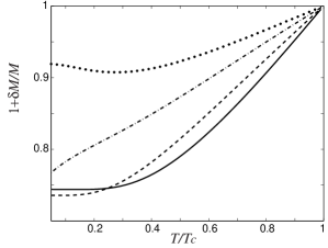
Figure 25: Change of the magnetization of a F/S bilayer as a function of the temperature.

It is interesting to calculate the total magnetic moment $\delta\bar{M}_{S}$ induced in the superconducting film and compare it with the total magnetization of the ferromagnet $M_{F0}d_{F}$ (as we have mentioned, the magnetization variation $\delta M_{F}$ in the ferromagnet is small and can be neglected).

The total magnetization of the superconductor is given by

$$\delta\bar{M}_{S}=\int_{-d_{s}}^{0}dx\delta M_{S}(x)\;.$$

Assuming that $h\ll\epsilon_{bF}=D_{F}/(2\gamma_{F}d_{F})$  or $h\ll[D_{F}/(2d_{F}^{2})](\rho_{F}d_{F}/R_{b})$, we can easily compute the ratio

$$\frac{\delta\bar{M}_{S}}{M_{F0}d_{F}}\approx-\pi\frac{D_{S}\nu_{S}\Delta^{2}T}{d_{F}\gamma_{S}\nu_{F}\epsilon_{bF}}\sum_{\omega}\frac{1}{(\omega^{2}+\Delta^{2})^{3/2}}=-1\;,$$ (146)

where $\rho_{F}$ is the resistivity of the F region.

We see that in the case of a thin ferromagnet at low temperatures and a not too strong exchange field the magnetization induced in the superconductor compensates completely the magnetization in the ferromagnet. This result follows from the fact that the magnetization induced in the superconductor (it is proportional to $g_{S3}$) spreads over distances of the order of $\xi_{S}$. In view of this result one can expect that the magnetic moment of a small ferromagnetic particle embedded in a superconductor should be completely screened by the Cooper pairs. We discuss the screening of a ferromagnet particle by the Cooper pairs in the next subsection.

It is worth mentioning that the problem of finding the magnetization in a $S/F$ structure consisting of thin $S$ ($d_{S}<\xi_{S}$) and $F$ ($d_{F}<\xi_{F}$) layers is equivalent to the problem of magnetic superconductors where ferromagnetic (exchange) interaction and superconducting correlations coexist. If we assume a strong coupling between the thin $S$ and $F$ layers, we can again average the equations over the thickness of the structure and arrive at the Usadel equation for the averaged Green’s function with an effective exchange field $\tilde{h}=hd_{F}/d$ and an effective order parameter $\tilde{\Delta}=\Delta d_{S}/d,$ where $d=d_{S}+d_{F}$. In this case the magnetization is given by $M=g\mu_{B}\nu\sqrt{\tilde{h}^{2}-\tilde{\Delta}^{2}}\Theta(\tilde{h}-\tilde{\Delta})$, where  $\Theta\left(x\right)$  is the step function. This means that the total magnetization $M$ is zero for $\tilde{h}<\tilde{\Delta}$. This result agrees with those obtained by Karchev et al. (2001); Shen et al. (2003) who studied the problem of the coexistence of superconductivity and itinerant ferromagnetism in magnetic superconductors.

One of the assumptions made for obtaining the previous results is the quasiclassical condition $h/\epsilon_{F}\ll 1$. For some materials the latter is not fulfilled and one has to go beyond the quasiclassical approach. Halterman and Valls (2002a) studied the imbalance of spin up and spin down electrons in pure $S/F$ structures (i.e. without impurities) in the case of strong exchange fields ($h/\epsilon_{F}\leq 1$). In that case superconductivity is strongly suppressed at the $S/F$ interface. Solving the Bogoliubov-de Gennes equations numerically the authors showed that there was a magnetic “leakage” from the ferromagnet into the superconductor, which lead to a polarization of the electrons in $S$ over the short length scale $\lambda_{F}$. The direction of the induced magnetic moment in the superconductor was parallel to that in the ferromagnet, which contrasts our finding.

At the same time, the limit of a very strong exchange field considered by Halterman and Valls (2002a) differs completely from ours. It is clear that due to the strong suppression of the superconductivity at the $S/F$ interface, the magnetic moment cannot be influenced by the superconductivity and therefore thick ferromagnetic layers with exchange energies of the order of the Fermi energy are not suitable for observing the reduction of the magnetization described above.

The DOS for states with spin-up and spin-down electrons in a $S/F$ structure has been calculated on the basis of the Usadel equation by Fazio and Lucheroni (1999). The authors have found that the DOS of these states was different in the superconductor over the length of the order $\xi_{S}$. However, the change of the magnetization has not been calculated in this work.

This has been done later by Krivoruchko and Koshina (2002) for a $S/F$ structure. Using the Usadel equation, the authors numerically calculated the magnetization induced in the superconductor. They found that the magnetic moment leaked from the $F$ layer into the $S$ layer and changed the sign at some distance of the order of $\xi_{S}$, thus becoming negative at sufficiently large distances only. In our opinion, the “leakage” of the magnetic moment $M_{S}$ obtained in that paper is a consequence of the use by the authors of a wrong expression for the magnetic moment. They did not add to the formula obtained in the quasiclassical approximation a contribution from the energies levels located far from the Fermi energy. The latter contribution is not captured by the quasiclassical approach and should be written additionally.

We have seen that under certain conditions a finite magnetic moment is induced inside the superconductor. Does this magnetic moment affect the superconductivity? The magnetic field $B_{S}$ in the superconductor equals the magnetization $4\pi M_{s}$. The induced magnetization in the superconductor $M_{S}$ is smaller than the magnetization in the ferromagnet: $M_{S}=M_{F}\max(d_{F}/\{\xi_{S},d_{S}\})$. The critical field for superconducting thin films is given by the expression $H_{c}\sim(\lambda_{L}/d_{S})H_{bulk}$, where $\lambda_{L}$ is the London penetration depth, and $H_{bulk}$ is the critical field of the bulk material. The superconductivity is not affected by the induced field $B_{S}$ if the field $B_{S}\approx 4\pi M_{F}(d_{F}/\xi_{S})$ (we set $d_{S}\approx\xi_{S}$) is smaller than $H_{c}$. Therefore the condition $4\pi M_{F}<(\lambda_{L}/d_{F})H_{bulk}$ should be satisfied. If we take $\lambda_{L}\approx 1\mu m$ and $d_{F}\approx 50$Å, we arrive at the condition $4\pi M_{F}<200H_{bulk}$. This condition is fulfilled easily for the case of not too strong ferromagnets. Due to the presence of the magnetization in the ferromagnet and superconductor spontaneous currents arise in the system. The spontaneous Meissner currents induced by the magnetization in S/F structures were studied by Bergeret et al. (2001c); Krawiec et al. (2004).

The phenomenon discussed in this section can be considered as an alternative mechanism of the decrease of the total magnetic moment observed by Garifullin et al. (2002). In order to clarify which of these two effects is more important for the experimental observations one needs more information.

The most direct check for the cryptoferromagnetic phase would be measurements with polarized neutrons. In a recent work by Stahn et al. (2005), in which a multilayered $S/F/S/F...$ structure was studied. This structure consists of the high $T_{c}$ superconductor $YBa_{2}Cu_{3}O_{7}$ ($S$ layer) and of the ferromagnet $La_{2/3}Ca_{1/3}MnO_{3}$ ($F$ layer). Two samples with the $S$ and $F$ layers of the same thickness were used. Layers of sample 1(2) are $98$Å($160$Å) thick. The Curie temperature of the ferromagnet and the temperature of the superconducting transition are equal to $165K$ and $75K$ respectively. By using neutron reflectometry the authors obtained an information about the spatial distribution of the magnetic moment in the structure. Analyzing the temperature dependence of the Bragg peaks intensity they came to the conclusion that the most probable scenario to explain important features of this dependence observed was the assumption that an induced magnetization arises in the $S$ layers. If this explanation was correct, the sign of the induced magnetization had to be opposite to the sign of the magnetization in the $F$ layers. It is quite reasonable to think that the mechanism discussed above for conventional superconductors should be present also in high $T_{c}$ superconductors and then the theoretic scenario analyzed in this section can serve as an explanation of the experiment.

V.3 Spin screening of the magnetic moment of a ferromagnetic particle in a superconductor

Let us  consider now a ferromagnetic particle (grain) embedded into a superconductor (see FIG. 26). As in the previous subsection, we analyze the magnetic moment induced in the superconductor around the particle and compare it with the magnetic moment of the $F$ particle $(4\pi a^{3}/3)M_{F0}$ (we assume that the particle has a spherical form and radius $a$).

Figure 26: Ferromagnetic grain embedded into a superconductor. Due to the inverse proximity effect the magnetic moment of the grain is screened by the electrons of the superconductor.

It is well known that the superconducting currents (Meissner currents) in a superconductor screen a magnetic field that decays from the surface over the London penetration length $\lambda_{L}$ and vanishes in the bulk of the superconductor. The same length characterizes the decay of the magnetic field created by a ferromagnetic $(F)$ grain embedded in a superconductor if the radius  of the grain $a$ is larger than $\lambda_{L}$. However, if the radius $a$ is small, the Meissner effect can be neglected and a stray magnetic field around the grain should decay, as in a normal metal, over a length of the order $a$. We consider now just this case.

Above the critical temperature $T_{c}$ the stray magnetic field polarizes the spins of free electrons and induces a magnetic moment. This magnetic moment is very small because the Pauli paramagnetism is weak ($\mu_{B}^{2}\nu\sim 10^{-6}$). In addition, the total magnetic moment induced by the stray magnetic field is zero. The penetration depth $\lambda_{L}$ can be of the order of hundreds of interatomic distances or larger, so that if $a$ is smaller or of the order of $10nm$, the Meissner effect can be neglected.

The screening of the magnetic moment is a phenomenon specific for superconductors. It is usually believed that in a situation, when the screening due to the orbital electron motion can be neglected (small grains and thin films), the total magnetic moment is just the magnetic moment of the ferromagnetic particle and no additional magnetization is induced by the electrons of the superconductor.

This common wisdom is quite natural because in conventional superconductors the total spin of a Cooper pair is equal to zero and the polarization of the conduction electrons is even smaller than in the normal metal. Spin-orbit interactions may lead to a finite magnetic susceptibility of the superconductor but it is positive and smaller anyway than the one in the normal state Abrikosov and Gor’kov (1962); Abrikosov (1988).

Let us now take a closer look at the results of the last subsection. We have seen that the proximity effect induces in the superconductor a magnetic moment with the sign opposite to the one in the ferromagnet. In view of this result it is quite natural to expect that the magnetic moment of a small ferromagnetic particle embedded in a superconductor may be screened by the Cooper pairs as it is sketched in FIG. 26. So, let us consider this situation in more detail.

We consider a ferromagnetic grain of radius $a$ embedded in a bulk superconductor. If the size of the particle is smaller than the length $\xi_{F}$ we can again assume that the quasiclassical  Green’s functions in the $F$ region are almost constant and given by Eq. (144), where now $\epsilon_{bF}=3D_{F}/(2\gamma_{F}a)$. In the superconductor we have to solve the linearized Usadel equation for the component $g_{S3}$ determining the magnetization

$$\nabla^{2}g_{S3}-\kappa_{S}^{2}g_{S3}=0\;,$$ (147)

where $\nabla^{2}=\partial_{rr}+(2/r)\partial_{r}$ is the Laplace operator in spherical coordinates.

Using the boundary conditions Eq. (181) we write the solution of this equation as

$$g_{S3}=\frac{f_{BCS}}{\gamma_{S}}\left(g_{BCS}f_{F0}-f_{BCS}g_{F3}\right)\frac{a^{2}}{1+\kappa_{S}a}\frac{e^{-\kappa_{S}(r-a)}}{r}\;,$$ (148)

where $f_{F0}=(f_{F+}+f_{F-})/2$ and $g_{F3}=(g_{F+}-g_{F-})/2$.

We assume again that the transmission coefficient through the $S/F$ interface is not small and the condition $\Delta<<h\leq(D_{F}/a^{2})$ is fulfilled. In this case the expression for $g_{S3}$ drastically simplifies. Indeed, in this limit $g_{F3}=f_{F0}f_{BCS}/g_{BCS}$ and $f_{F0}\cong ihf_{BCS}g_{BCS}/\epsilon_{bF}$. Therefore Eq.(148) acquires the form

$$\mathbf{g}_{S3}\mathbf{=}\frac{f_{BCS}^{2}}{\gamma_{S}}\frac{a^{2}}{r}\frac{ih}{\epsilon_{bF}}\mathbf{e}^{-\kappa_{S}(r-a)}\mathbf{\;,}$$ (149)

This solution can be obtained from Eq.(147) if one writes down the term $4\pi A\delta(r)$ on the right-hand side of this equation with $A=f_{BCS}^{2}a^{2}ih/(\gamma_{S}\epsilon_{bF}).$ This means that the ferromagnetic grain acts on Cooper pairs as a magnetic impurity embedded into a dirty superconductor. It induces a ferromagnetic cloud of the size of the order $\xi_{S}$ with a magnetic moment $\sim-\mu_{B}\nu hV_{F}.$

In order to justify the assumptions made above we estimate the energy $D_{F}/a^{2}$ assuming that the mean free path is of the order of $a$. For $a=30$Å and $v_{F}=10^{8}cm/\sec$ we get $D_{F}/a^{2}\sim 1000K;$. This condition is fulfilled for ferromagnets with the exchange energy of the order of several hundreds $K$.

In the limit of  low temperatures the calculation of the magnetic moment becomes very easy and we obtain for the magnetic moment $\bar{M}_{S}$ induced in the superconductor the following expression

$$\frac{\bar{M}_{S}}{M_{F0}(4\pi a^{3}/3)}=-1$$ (150)

This is a remarkable result which shows that the induced magnetic moment is opposite in sign to the moment of the ferromagnetic particle and their absolute values are equal to each other. In other words, the magnetic moment of the ferromagnet is completely screened by the superconductor Bergeret et al. (2004b). The characteristic radius of the screening is the coherence length $\xi_{S}$, which contrasts the orbital screening due to the Meissner effect characterized by the London penetration depth $\lambda_{L}$.

To avoid misunderstanding we emphasize once again that the full screening occurs only if the magnetization (per unit volume) of the ferromagnetic grain $M_{F0}$ is given by Eq.(139), which means that the ferromagnetic grain is an itinerant ferromagnet. If the magnetization of the ferromagnet is caused by both localized moments ($M_{loc})$ and itinerant electrons ($M_{itin})$, the full screening is not achieved. Moreover, the magnetization $M_{loc}$ may be larger than $M_{itin}$ and have opposite direction. In this case we would have an anti-screening Bergeret and García (2004).

Actually, we have discussed the diffusive case only. However, it turns out that the spin screening occurs also in the clean case provided the exchange field is not too high: $h<<v_{F}/d_{F}$, where $v_{F}$ and $d_{F}$ are the Fermi velocity and the thickness (radius) of the ferromagnetic film or grain Kharitonov et al. (2005); Bergeret et al. (2005).

The energy spectrum of a superconductor with a point-like classical magnetic moment was studied many years ago by Shiba (1968), Sakurai (1970) and Rusinov (1969), and more recently by Salkola et al. (1997). The magnetic impurity leads to a bound state $\beta_{0}$ inside the superconducting energy gap. There is some critical strength $h_{c}\sim\epsilon_{F}$ of the exchange coupling $h$ that separates two different ground states of the system denoted by $\psi$ if $h<h_{c}$ and $\psi^{\prime}$ if $h>h_{c}$. The bound state $\beta_{0}$ corresponds to a localized quasiparticle with spin “up”. Since the total electronic spin in the state $\psi$ is zero one says that the continuum localizes a spin “up”. The energy needed to create a quasiparticle excitation decreases when increasing $h$. At $h=h_{c}$ the state $\psi$ becomes unstable against a spontaneous creation of an excitation with spin “up” and the transition to the state $\psi^{\prime}$ occurs. In this state the electronic spin at the impurity site is now equal to $-1/2$. All the works considering this problem focused the attention on the subgap structure of the spectrum and did not addressed the problem of the screening of the magnetic moment by the continuum spectrum. This is of no surprise because a sufficiently large magnetic moment of the impurity ($S\gg 1$) cannot be screened by the quasiparticles.

V.4 Spin-orbit interaction and its effect on the proximity effect

In this section we discuss the influence of the spin-orbit (SO) interaction on the proximity effect. Although in general its characteristic energy scale is much smaller than the exchange energy $h$, it can be comparable with the superconducting gap $\Delta$ and therefore this effect can be very important. Since the SO scattering leads to a mixing of the spin channels, we expect that it will affect not only the singlet component of the condensate but also the triplet one in the ferromagnet.

In conventional superconductors the SO interaction does not affect thermodynamic properties. However, a non-vanishing magnetic susceptibility at zero temperature (Knight shift) observed in small superconducting samples and films can be explained only if the SO interaction is taken into account Abrikosov and Gor’kov (1962). In the $F/S$ structures considered here the exchange field $h$ breaks the time-reversal symmetry in analogy to the external magnetic field in the Knight shift problem. Therefore the SO interaction in the superconductor is expected to influence the inverse proximity effect studied in this Chapter.

In this Section we will generalize the analysis of the long-range proximity effect and the inverse proximity effect presented above taking the SO interaction into account. The quasiclassical equations in the presence of the SO interaction were derived by Alexander et al. (1985) and used for the first time for the $F/S$ systems by Demler et al. (1997).

The derivation of these equations is presented in the Appendix A. The resulting Usadel equation takes the form

$$-iD\partial_{\mathbf{r}}(\mbox{$\check{g}$}\partial_{\mathbf{r}}\mbox{$\check{g}$}) + i\left(\mbox{$\hat{\tau}_{3}$}\partial_{t}\mbox{$\check{g}$}+\partial_{t^{\prime}}\mbox{$\check{g}$}\mbox{$\hat{\tau}_{3}$}\right)+\left[\check{\Delta},\mbox{$\check{g}$}\right]+\left[\mathbf{h}\mathbf{\check{S}},\mbox{$\check{g}$}\right]$$ (151)

$$+ \frac{i}{\tau_{s.o.}}\left[\mathbf{\check{S}}\mbox{$\hat{\tau}_{3}$}\mbox{$\check{g}$}\mbox{$\hat{\tau}_{3}$}\mathbf{\check{S}},\mbox{$\check{g}$}\right]=0\;.$$

All symbols are defined in the Appendix A. The spin-orbit relaxation time $\tau_{s.o.}$ takes very different values depending on the material used in the experiments. Some estimates for the values of $1/h\tau_{s.o.}$can be found in Oh et al. (2000). For example, for transition metals like $Fe$ one obtains $1/h\tau_{s.o.}\sim 10^{-2}$, while for a typical magnetic rare earth the value  $1/h\tau_{s.o.}\sim 0.3$ is more typical. In the latter case the SO interaction should clearly affect the penetration of the condensate into the ferromagnet.

In order to study the influence of the SO interaction on both the long-range and the inverse proximity effect we will use Eq.(151). We consider first the well known problem of the Knight shift. This example will show the convenience of using the quasiclassical approach.

The Knight shift in superconductors

Since the pioneering work of Abrikosov and Gor’kov (1962) it is well established that the magnetic susceptibility of small superconducting samples is not zero due to the spin-orbit interaction. This explains the experiments performed for the first time many years ago by Androes and Knight (1961) who used the nuclear magnetic resonance technique.

Let us consider a superconductor in an external magnetic field $H$. In the Usadel equation, Eq. (151), the field $H$ plays the role of the exchange energy $h$. We are interested in the linear response to this filed, i.e. in the magnetic susceptibility $\chi_{S}$ of the superconductor. We assume that the superconductor is homogeneous and therefore we drop the gradient term in Eq. (151):

$$-\omega\left[\hat{\tau}_{3},\check{g}\right]+i\left[\check{\Delta},\mbox{$\check{g}$}\right]+iH\left[\check{n},\mbox{$\check{g}$}\right]-({1}/\tau_{s.o.})\left[\mathbf{\check{S}}\mbox{$\hat{\tau}_{3}$}\mbox{$\check{g}$}\mbox{$\hat{\tau}_{3}$}\mathbf{\check{S}},\mbox{$\check{g}$}\right] = 0\;,$$ (152)

$$\check{g}^{2} = 1\;.$$ (153)

The solution of Eq. (152) has the form

$$\check{g}=\left(g_{BCS}+g_{3}\hat{\sigma}_{3}\right)\hat{\tau}_{3}+\left(f_{BCS}\hat{\sigma}_{3}+f_{0}\right)i\hat{\tau}_{2}\;,$$ (154)

where the functions $g_{3}$ and $f_{0}$ are corrections to the normal $g_{BCS}$ and anomalous $f_{BCS}$ Green’s functions. In the particle-hole space the matrix $\check{g}$ has the usual form, i.e. it is expanded in matrices $\hat{\tau}_{3}$ and $i\mbox{$\hat{\tau}_{2}$}$. In the spin space the triplet component (the $g_{3}$ and $f_{0}$ terms) appears due to the magnetic field acting on the spins. Using Eqs. (152-154) one can readily obtain

$$g_{3}=-i\frac{\Delta^{2}H}{E_{\omega}^{2}(E_{\omega}+4/\tau_{s.o.})}\;.$$ (155)

where $E_{\omega}=\sqrt{\Delta^{2}+\omega^{2}}$.

Substituting Eq. (155) into Eq. (145) we can write the magnetization $M$ as follows

$$M=M_{0}-\mu_{B}\nu\left(2\pi T\Delta^{2}\sum_{\omega}\frac{1}{E_{\omega}^{2}(E_{\omega}+4/\tau_{s.o.})}\right)H$$ (156)

The first term in Eq. (156) cannot be calculated in the framework of the quasiclassical theory and one should use exact Green’s functions. It corresponds to the Pauli paramagnetic term given by $M_{0}=\mu_{B}\nu H$. In the quasiclassical approach this term is absent. This term does not depend on temperature on the energy scale of the order of $T_{c}$ and originates from a contribution of short distances where the quasiclassical approximation fails.

This situation is rather typical for the quasiclassical approach and one usually adds to formulae obtained within this approach contributions coming from short distances or times by hand (see, for example, Artemenko and Volkov (1980); Kopnin (2001); Rammer and Smith (1986)). Eq. (156) was first obtained by Abrikosov and Gor’kov (1962).

In the absence of the spin orbit interaction the magnetization at $T=0$ is, as expected, equal to zero. However, if the SO interaction is finite the spin susceptibility $\chi_{S}$ does not vanish at $T=0$. It is interesting that, as follows from Eq. (152), the singlet component of the condensate is not affected by the SO interaction. The origin of the finite susceptibility is the existence of the triplet component $f_{0}$ of the condensate.

In the $S/F$ structures there is no exchange field in the superconductor and therefore the situation is in principle different. However, we have seen that due to the proximity effect the triplet component $f_{0}$ is induced in the superconductor.

From the above analysis one expects that the SO interaction may affect the penetration length of such component in the superconductor. In the next sections we consider the influence of the SO the superconducting condensate in both the ferromagnet and the superconductor.

V.4.1 Influence of the Spin-Orbit interaction on the long-range Proximity Effect

Now we consider again the $S/F/S/F/S$ structure of Section IV.1 and assume that the long-range triplet component is created, which is possible provided the angle $\alpha$ between the magnetizations differs from $0$ and $\pi$. In order to understand how the SO interaction affects the triplet component it is convenient to linearize Eq. (151) in the $F$-layer assuming, for example, that the proximity effect is weak. One can easily obtain a linearized equation similar to Eq. (52) for the condensate function $\check{f}$. The solution of this equation is represented again in the form

$$\mbox{$\check{f}$}(x)=i\mbox{$\hat{\tau}_{2}$}\otimes(f_{0}(x)\mbox{$\hat{\sigma}_{0}$}+f_{3}(x)\mbox{$\hat{\sigma}_{3}$})+i\mbox{$\hat{\tau}_{1}$}\otimes f_{1}(x)\mbox{$\hat{\sigma}_{1}$}\;.$$ (157)

The functions $f_{i}(x)$ are given as before  by $f_{i}(x)=\sum_{j}b_{j}\exp[\kappa_{j}x]$ but now the new eigenvalues $\kappa_{j}$ are written as

$$\kappa_{\pm}^{2} = \pm\frac{2i}{D_{F}}\sqrt{h^{2}-\left(\frac{4}{\tau_{so}}\right)^{2}}+\frac{4}{\tau_{so}D_{F}}$$ (158)

$$\kappa_{0}^{2} = \kappa_{\omega}^{2}+2\left(\frac{4}{\tau_{s.o.}D_{F}}\right)\;.$$ (159)

We see from these equations that both the singlet and triplet components are affected by the spin-orbit interaction making the decay of the condensate in the ferromagnet faster. In the limiting case, when  $4/\tau_{so}>h,T_{c}$, both the components penetrate over the same distance $\xi_{s.o.}=\sqrt{\tau_{so}D_{F}}$ and therefore the long-range effect is suppressed. In this case the characteristic oscillations of the singlet component are destroyed Demler et al. (1997). In the more interesting case $4/\tau_{so}\sim T_{c}<h$, the singlet component does not change and penetrates over the short distance $\xi_{F}$ . At the same time, the triplet component is more sensitive to the spin-orbit interaction and the penetration length equals $\min$($\xi_{so},\xi_{T}$)$>\xi_{F}$.

Therefore, if the spin-orbit interaction is not very strong, the penetration of triplet condensate over the long distances discussed in the preceding sections is still possible, although the penetration length is reduced.

V.4.2 Spin-Orbit Interaction and the Inverse Proximity Effect

Studying a $S/F$ bilayer we have seen that the induced magnetic moment in the superconductor $S$ is related to the appearance of the triplet component $f_{0}$. Moreover, we have shown that this component is affected by the SO interaction, while the singlet one $f_{3}$ is not. So, one should expect that the SO interaction may change the scale over which the magnetic moment is induced in the superconductor and one can estimate easily this length.

Assuming that the Green’s functions in the superconductor take values close to the bulk values we linearize the Usadel equation (151) in the superconductor. The solution has the same form as before, Eq. (143), but $\kappa_{S}$ should be replaced by

$$\kappa_{S}^{2}\rightarrow\kappa_{S}^{2}+\kappa_{so}^{2},$$ (160)

where $\kappa_{so}^{2}=8D_{S}/\tau_{so}$. Therefore, the length of the penetration of $g_{S3}$ and, in its turn, of  $M_{S}$ into the $S$ region decreases if $\kappa_{S}^{2}\sim\xi_{S}^{-2}<\kappa_{so}^{2}$.

In principle, one can measure the spatial distribution of the magnetic moment in the $S$ region as it was done by Luetkens et al. (2003) by means of muon spin rotation and get an information about the SO interaction in superconductors. As Eq. (160) shows, this would be an alternative method to measure the strength of the SO interaction in superconductors, complementary to the measurement of the Knight shift Androes and Knight (1961).

VI Discussion of the results and outlook

In this review we have discussed new unusual properties of structures consisting of conventional superconductors in a contact with ferromagnets. It has been known that such systems might exhibit very interesting properties like a non-monotonous reduction of the superconducting temperature as a function of the thickness of the superconductor, possibility of a $\pi$-contact in Josephson junctions with ferromagnetic layers, etc.

However, as we have seen, everything is even more interesting and some spectacular phenomena are possible that even might look at first glance as a paradox. The common feature of the effects discussed in this review is that almost all of them originate in situations when the exchange field is not homogeneous. As a consequence of the inhomogeneity, the spin structure of the superconducting condensate function becomes very non-trivial and, in particular, the triplet components are generated. In the presence of the inhomogeneous exchange field, the total spin of a Cooper pair is not necessarily equal to zero and the total spin equal to unity with all projections onto the direction of the exchange field is possible.

We have discussed the main properties of the odd triplet superconductivity in the $S/F$ structures. This superconductivity differs from the well known types of superconductivity: a) singlet superconductivity with the s-wave (conventional $T_{c}$ superconductors) and d-wave (high $T_{c}$ superconductors) types of pairing; b) odd in momentum $p$ and even in frequency $\omega$ triplet superconductivity observed, e.g., in $Sr_{2}RuO_{4}$.

The odd triplet superconductivity discussed in this Review has a condensate (Gor’kov) function that is an odd function of the Matsubara frequency $\omega$ and an even function (in the main approximation) of the momentum $p$ in the diffusive limit. It is insensitive to the scattering on nonmagnetic impurities and therefore may be realized in thin film $S/F$ structures where the mean free path is very short.

For the first time, the condensate function of this type has been suggested by Berezinskii (1975) many years ago as a possible candidate to describe superfluidity in $He^{3}$. Later, it has been established  that the superfluid condensate in $He^{3}$ had a different structure - it was odd in $p$ and even in $\omega$. In principle, there is an important difference between the triplet superconductivity discussed here and that predicted by Berezinskii who assumed that the order parameter $\Delta$ was also an odd function of $\omega$. In our case the order parameter $\Delta$ is determined by the singlet, s-wave condensate function and has the ordinary BCS structure (i.e., it does not depend on the momentum $p$ and frequency $\omega$). On the other hand the structure of the triplet condensate function $\;\check{f}$ in the diffusive case considered here  coincides with that suggested by Berezinskii: it is an odd function of the Matsubara frequency $\omega$ and, in the main approximation, is constant in the momentum space. The antisymmetric part of $\;\check{f}$  is small compared with the symmetric part,  being odd in $p$ and even in $\omega.$

The triplet component with the projection of the total spin $S_{z}=\pm 1$ penetrates the ferromagnet over a long distance of the order of $\xi_{N}\approx\sqrt{D_{F}/2\pi T},$ which shows that the exchange field does not affect the triplet part of the condensate.  At the same time, the exchange field suppresses the amplitude of the singlet component at the $S/F$ interface that determines the amplitude of the triplet component. The long-range triplet component arises only in the case of a nonhomogeneous magnetization. The triplet component appears also in a system with a homogeneous magnetization but in this case it corresponds to the projection $S_{z}=0$ and penetrates the ferromagnet over a short length $\xi_{F}=\sqrt{D_{F}/h}<<\xi_{N}$.

The triplet component exists also in magnetic superconductors Bulaevskii et al. (1985); Kulic and Kulic (2001) with a spiral magnetic structure. However, it always coexists with the singlet component and cannot be separated from it. In contrast, in the  multilayered $S/F$ structures with a nonhomogeneous magnetization and with the thickness of the $F$ layers $d_{F}$ exceeding $\xi_{F}$, the Josephson coupling between $S$ layers is realized only through the long-range triplet component and this separates the singlet and triplet components from each other. As a result, the “real” odd triplet superconductivity may be realized in the transverse direction in such structures.

Another interesting peculiarity of the $S/F$ structures is the inverse proximity effect, namely, the penetration of the magnetic order parameter (spontaneous magnetic moment $M$) into the superconductor and a spatial variation of the magnetization direction in the ferromagnet under the influence of the superconductivity. It turns out that both effects are possible. A homogeneous distribution of the magnetization $M_{F}$ in the $S/F$ bilayer structures may be energetically unfavorable in $F$ even in a one-domain case resulting in a nonhomogeneous distribution of $\mathbf{M}_{F}$ in the ferromagnet.

Moreover, the magnetic moment penetrates the superconductor (induced ferromagnetism) changing sign at the $S/F$ interface. Therefore the total magnetic moment of the system is reduced. Under some condition the full spin screening of $M_{F}$ occurs. For example, at zero temperature the itinerant magnetic moment of a ferromagnetic grain embedded into a superconductor is completely screened by spins of the Cooper pairs in $S$. The radius of the screening cloud is of the order of the superconducting coherence length $\xi_{S}$. If the magnetization vector $\mathbf{M}_{F}$ is oriented in the opposite direction to the ferromagnetic exchange field $\mathbf{h}$, the anti-screening is possible.

As concerns the experimental situation, certainly there are indications in favor of the long-range triplet component, although an unambiguous evidence does not exist so far. For example, the resistance of ferromagnetic films or wires in the $S/F$ structures changes on distances that exceed the length of the decay of the singlet component $\xi_{h}$ Aumentado and Chandrasekhar (2001); Petrashov et al. (1999); Giroud et al. (1998). A possible reason for this long-range proximity effect in the $S/F$ systems is the long-range penetration of the triplet component. However a simpler effect might also be the reason for this long-range proximity effect. It is related to a rearrangement of a domain structure in the ferromagnet when the temperature lowers below $T_{c}$. The Meissner currents induced in the superconductor by a stray magnetic field affect the domain structure, and the resistance of the ferromagnet may change Dubonos et al. (2002). At the same time, the Meissner currents should be considerably reduced in an one dimensional geometry for the ferromagnet like that used in Giroud et al. (1998) and the explanation in terms of the long range penetration of the triplet component are more probable here.

Sefrioui et al. (2003) also obtained some indications on the existence of a triplet component in a multilayered $S/F/S/F$… structure. The samples used by Sefrioui et al. contained the high $T_{c}$ material $YBa_{2}Cu_{3}O_{7}$ (as a superconductor) and the half-metallic ferromagnet $La_{0.7}Ca_{0.3}MnO_{3}$ (as a ferromagnet). They found that superconductivity persisted even in the case when the thickness of the $F$ layers $d_{F}$ essentially exceeded $\xi_{F}$ ($d_{F}\gtrsim 10nm$ and $\xi_{F}\approx 5nm$). In a half-metal ferromagnet with spins of free electrons aligned in one direction the singlet Cooper pairs cannot exist. Therefore it is reasonable to assume that the superconducting coupling between neighboring $S$ layers is realized via the triplet component Volkov et al. (2003); Eschrig et al. (2003).

A reduction of the magnetic moment of the $S/F$ structures due to superconducting correlations  has been observed already Garifullin et al. (2002). This reduction may be caused both by the spin screening of the magnetic moment $M_{F}$ and by the rotation of $M_{F}$ in space Bergeret et al. (2000); Bergeret et al. (2004a). Perhaps, the spin screening can be observed directly by probing the spatial distribution of the magnetic field (or magnetic moment $M$) with the aid of the muon spin rotation  technique Luetkens et al. (2003). The variation of the magnetic moment $M$ occurs on a macroscopic length $\xi_{S}$ and therefore can be detected.

An evidence in favor of the inverse proximity effect has also been obtained in another experimental work Stahn et al. (2005). Analyzing data of neutron reflectometry on a multilayered $YBa_{2}Cu_{3}O_{7}/La_{2/3}Ca_{1/3}MnO_{3}$ structure, the authors concluded that a magnetic moment was induced in the superconducting $YBa_{2}Cu_{3}O_{7}$ layers. The sign of this induced moment was opposite to the sign of the magnetic moment in the ferromagnetic $La_{2/3}Ca_{1/3}MnO_{3}$ layers, which correlates with our prediction.

In spite of these experimental results that may be considered as, at least preliminary, confirmation of the existence of the triplet component in the $S/F$ structures, there is a need in additional experimental studies of the unconventional superconductivity discussed in this review. One of the important issues would be to understand whether the long range proximity effects already observed experimentally are due to the triplet pairing or to a simple redistribution of the domain walls by the Meissner currents. We believe that measurements on thin ferromagnetic wires where the Meissner currents are reduced may clarify the situation.

It is very interesting to distinguish between the two possible inverse proximity effects experimentally. Although both the formation of the cryptoferromagnetic state and the induction of the magnetic moments in the superconductors are very interesting effects, it is not clear yet which of these effects causes the magnetization reduction observed by Mühge et al. (1998); Garifullin et al. (2002).

The enhancement of the Josephson current by the presence of the ferromagnet near the junction is one more theoretical prediction that has not been observed yet but, certainly, this effect deserves an attention. An overview for experimentalists interested in all these subjects is presented in Appendix B, where we discuss briefly different experiments on S/F structures, focusing our attention on the materials for which, we expect, the main effects discussed in this review may be observed.

In addition, further theoretical investigations are needed. The odd triplet component has been studied mainly in the diffusive limit ($h\tau<<1$). It would be interesting to investigate the properties of the triplet component for an arbitrary impurity concentration ($h\tau\gtrless 1$). No theoretical work on dynamics of magnetic moments in the $S/F$ structures has been performed yet, although the triplet component may play a very important role in the dynamics of the $S/F$ structures. Transport properties of the $S/F$ structures require also further theoretical considerations. It would be useful to study the influence of domain structures on properties of the $S/F$ structures, etc. In other words, physics of the proximity effects in the superconductor-ferromagnet structures is evolving into a very popular field of research, both experimentally and theoretically.

The study of the proximity effect in $S/F$ structures may be extended to include ferromagnets in contact with high temperature superconductors. Although some experiments have been done already Sefrioui et al. (2003); Stahn et al. (2005), one can expect much more broad experimental investigations in the future. The modern technique allows the preparation of multilayered $S/F/S/F$.. structures consisting of thin ferromagnetic layers (as $La_{2/3}Ca_{1/3}MnO_{3}$) and thin layers of high $T_{c}$ superconductor (as $YBa_{2}Cu_{3}O_{7}$) with variable thicknesses. It would be very interesting to study, both experimentally and theoretically, such a system with non-collinear magnetization orientations. In this case d-wave singlet and odd triplet superconductivity should coexist in the system. It is known that many properties of the ordinary BCS superconductivity remain unchanged in the high $T_{c}$ superconductors. This means that many effects considered in this review can also occur in S/F structures containing high $T_{c}$ materials, but there will certainly be differences with respect to the conventional superconductors with the s-pairing.

We hope that this review will encourage experimentalists and theoreticians to make further investigations in this fascinating field of research.

Appendix A Basic equations

Throughout this review we use mainly the well established method of quasiclassical Green’s functions. Within this method the Gor’kov equations can be drastically simplified by integrating the Green’s function over the momentum. This method was first introduced by Larkin and Ovchinnikov (1968) and Eilenberger (1968), and then extended by Usadel (1970) for a dirty case and by Eliashberg (1971) for a non-equilibrium case . The method of the quasiclassical Green’s functions is discussed in many reviews Serene and Reiner (1983); Rammer and Smith (1986); Larkin and Ovchinnikov (1984); Belzig et al. (1999) and in the book by Kopnin (2001). In this Appendix we present a brief derivation of equations for the quasiclassical Green’s functions and write formulae for the main observable quantities in terms of these functions. A special attention will be paid to the dependence of these functions on the spin variables that play a crucial role in the S/F structures. In particular, we take into account the spin-orbit interaction alongside with the exchange interaction in the ferromagnet.

We start with a general Hamiltonian describing a conventional BCS-superconductor/ferromagnet structure:

$$\hat{H} = \sum_{\{p,s\}}\left\{a_{sp}^{+}\left[\left(\left(\xi_{p}\delta_{pp^{\prime}}+eV\right)+U_{imp}\right)\delta_{ss^{\prime}}+U_{s.o.}\right.\right.$$ (161)

$$\left.\left.-\left(\mathbf{h}.\sigma\right)\right]a_{s^{\prime}p^{\prime}}-\left(\Delta a_{\overline{s}\overline{p}}^{\dagger}a_{s^{\prime}p^{\prime}}^{\dagger}+c.c.\right)\right\}\;.$$

The summation is carried out over all momenta $(p,p^{\prime})$ and spins $(s,s^{\prime})$ (the notation $\overline{s}$, $\overline{p}$ means inversion of both spin and momentum), $\xi_{p}=p^{2}/2m-\epsilon_{F}$ is the kinetic energy counted from the Fermi energy $\epsilon_{F}$, $V$ is a smoothly varying electric potential. The superconducting order parameter $\Delta$ must be determined self-consistently. It vanishes in the ferromagnetic regions. The potential $U_{imp}=U(p-p^{\prime})$ describes the interaction of the electrons with nonmagnetic impurities, and $U_{s.o.}$ describes a possible spin-orbit interaction Abrikosov and Gor’kov (1962):

$$U_{s.o.}=\sum_{i}\frac{u_{s.o.}^{(i)}}{p_{F}^{2}}\left(\mathbf{p\times p^{\prime}}\right)\mathbf{\sigma}\;.$$

Here the summation is performed over all impurities.

The representation of the Hamiltonian in the form (161) implies that we use the mean-field approximation for the superconducting ($\Delta$) and magnetic ($\mathbf{h}$) order parameter. The exchange field $\mathbf{h}$ is parallel to the magnetization $\mathbf{M}_{F}$ in $F$. In strong ferromagnets the magnitude of $\mathbf{h}$ is much higher than $\Delta$ and corresponds to an effective magnetic field $H_{exc}=h/\mu_{B}$ of the order $10^{6}Oe$ (where $\mu_{B}=g\mu_{Bohr},$ $g$ is the $g$-factor and $\mu_{Bohr}$ is the Bohr magneton).

In order to describe the ferromagnetic region we use a simplified model that catches all physics we are interested in. Ferromagnetism in metals is caused by the electron-electron interaction between electrons belonging to different bands that can correspond to localized and conducting states. Only the latter participate in the proximity effect. If the contribution of free electrons strongly dominates (an itinerant ferromagnet), one has  $M_{F}\cong M_{e}$ and the exchange energy is caused mainly by free electrons.

If the polarization of the conduction electrons is due to the interaction with localized magnetic moments, the Hamiltonian $\hat{H}_{F}$ can be written in the form

$$\ \hat{H}_{F}=-h_{1}\sum_{\{p,s\}}\left\{a_{sp}^{+}\mathbf{S}\ast\mathbf{\sigma}_{ss^{\prime}}a_{s^{\prime}p^{\prime}}\right\}$$ (162)

where $\mathbf{S}=\sum_{a}\mathbf{S}_{a}\delta(r-r_{a})$, $\mathbf{S}_{a}$ is the spin of a particular ion. A constant $h_{1}$ is related to $h$ via the equation: $h=h_{1}n_{M}S_{0}$ , where $n_{M}$ is the concentration of magnetic ions and $S_{0}$ is a maximum value of $S_{a}$ (we consider these spins as classical vectors; see Ref. Gor’kov and Rusinov (1963)). In this case the magnetization is a sum: $M=M_{loc}+M_{e}$, and the magnetization $M_{e}$ can be aligned parallel ($h_{1}>0$, the ferromagnetic type of the exchange field)  to $M$ or antiparallel ($h_{1}<0$, the antiferromagnetic type of the exchange field). In the following we will assume a ferromagnetic exchange interaction ($M_{e}$ and $M$ are oriented in the same direction$)$. In principle,  one can add to Eq. (162) the term $\sum_{\{a,b\}}\left\{\mathbf{S}_{a}\ast\mathbf{S}_{b}\right\}$ describing a direct interaction between localized magnetic moments but in the most part of the review this term is not important except Section V.A. where the cryptoferromagnetic state is discussed.

Starting from the Hamiltonian (161) and using a standard approach Larkin and Ovchinnikov (1984), one can derive the Eilenberger and Usadel equations. Initially these equations have been derived for $2\times 2$ matrix Green’s functions $g_{n,n^{\prime}}$, where indices $n,n^{\prime}$ relate to normal $(g_{11},g_{22})$ and anomalous or condensate $(f_{12},f_{21})$ Green’s functions. These functions describe the singlet component. In the case of a non-homogenous magnetization considered in this review one has to introduce additional Green’s functions depending on spins and describe not only the singlet but also the triplet component. These matrices depend not only on $n,n^{\prime}$ indices but also on the spin indices $s,s^{\prime},$ and are $4\times 4$ matrices in the spin and Gor’kov space (sometimes the $n,n^{\prime}$ space is called the Nambu or Nambu-Gor’kov space).

In order to define the Green’s functions in a customary way it is convenient to write the Hamiltonian (161) in terms of new operators $c_{nsp}^{\dagger}$ and $c_{nsp}$ that are related to the creation and anhilation operators $a_{s}^{+}$ and $a_{s}$ by the relation (we drop the index $p$ related to the momentum)

$$c_{ns}=\left\{\begin{array}[]{c}a_{s},n=1\\ a_{\overline{s}}^{\dagger},n=2\;.\end{array}\right.$$ (163)

These operators (for $s=1$) were introduced by Nambu Nambu (1960) . The new operators allow one to express the anomalous averages $<a_{\uparrow}\cdot a_{\uparrow}>$ introduced by Gor’kov as the conventional averages $<c_{1}\cdot c_{2}^{+}>$ and therefore the theory of superconductivity can be constructed by analogy with a theory of normal systems. Thus, the index $n$ operates in the particle-hole (Numbs-Gor’kov) space, while the index $s$ operates in the spin space. In terms of the $c_{ns}$ operators the Hamiltonian can be written in the form

$$H=\sum_{\{p,n,s\}}c_{ns}^{+}\mathcal{H}_{(nn^{\prime})(ss^{\prime})}c_{n^{\prime}s^{\prime}}\;,$$ (164)

where the summation is performed over all momenta, particle-hole and spin indices. The matrix $\check{\mathcal{H}}$ is given by

$$\check{\mathcal{H}} = \frac{1}{2}\left\{\left[\left(\xi_{p}\delta_{pp^{\prime}}+eV\right)+U_{imp}\right]\hat{\tau}_{3}\otimes\hat{\sigma}_{0}+\widetilde{\hat{\Delta}}\otimes\hat{\sigma}_{3}-\mathbf{h}\hat{\tau}_{3}\mathbf{\check{S}}\right.$$ (165)

$$\left.+\sum_{i}\frac{u_{s.o.}^{(i)}}{p_{F}^{2}}\left(\mathbf{p\times p^{\prime}}\right)\mathbf{\check{S}}\right\}\;.$$

The matrices $\hat{\tau}_{i}$ and $\hat{\sigma}_{i}$ are the Pauli matrices in the particle-hole and spin space respectively; $i=0,1,2,3$, where $\hat{\tau}_{0}$ and $\sigma_{0}$ are the corresponding unit matrices. The matrix vector $\mathbf{\check{S}}$ is defined as

$$\mathbf{\check{S}}=(\hat{\sigma}_{1},\hat{\sigma}_{2},\hat{\tau}_{3}\hat{\sigma}_{3})\;,$$

and the matrix order parameter equals $\widetilde{\hat{\Delta}}=\hat{\tau}_{1}Re\Delta-\hat{\tau}_{2}Im\Delta$. Now we can define the matrix Green’s functions (in the particle-hole$\otimes$spin space) in the Keldysh representation in a standard way

$$\check{G}(t_{i},t_{k}^{\prime})=\frac{1}{i}\left\langle T_{C}\left(c_{ns}(t_{i})c_{n^{\prime}s^{\prime}}^{\dagger}(t_{k}^{\prime})\right)\right\rangle,$$ (166)

where the temporal indices take the values $1$ and $2$, which correspond to the upper and lower branch of the contour $C$, running from $-\infty$ to $+\infty$ and back to $-\infty$.

One can introduce a matrix in the Keldysh space of the form

$$\mathbf{\check{G}}(t,t^{\prime})=\left(\begin{array}[]{cc}\check{G}(t,t^{\prime})^{R}&\check{G}(t,t^{\prime})^{K}\\ 0&\check{G}(t,t^{\prime})^{A}\end{array}\right)$$ (167)

where the retarded (advanced) Green’s functions $\check{G}(t,t^{\prime})^{R(A)}$ are related to the matrices $\check{G}(t_{i},t_{k}^{\prime}):$ $\check{G}(t,t^{\prime})^{R(A)}=\check{G}(t_{1},t_{1}^{\prime})-\check{G}(t_{1(2)},t_{2(1)}^{\prime})$. All these elements are $4\times 4$ matrices. These functions determine thermodynamic properties of the system (density of states, the Josephson current etc). The matrix $\check{G}(t,t^{\prime})^{K}=$ $\check{G}(t_{1},t_{2}^{\prime})+\check{G}(t_{2},t_{1}^{\prime})$ is related to the distribution function and has a nontrivial structure only in a nonequilibrium case. In the equilibrium case it is equal to: $\check{G}(\epsilon)^{K}=\int d(t-t^{\prime})\check{G}(t-t^{\prime})^{K}\exp(i\epsilon(t-t^{\prime}))=[\check{G}(\epsilon)^{R}-\check{G}(\epsilon)^{A}]\tanh(\epsilon/2T).$

In order to obtain the equations for the quasiclassical Green’s functions, we follow the procedure introduced by Larkin and Ovchinnikov (1984). The equation of motion for the Green’s functions is

$$\left(i\partial_{t}-\check{H}-\check{\Sigma}_{imp}-\check{\Sigma}_{s.o.}\right)\mathbf{\check{G}}=\check{1}\;,$$ (168)

where

$$\check{H}=-\mbox{$\hat{\tau}_{3}$}\frac{\partial_{\mathbf{r}}^{2}}{2m}-\epsilon_{F}-\mathbf{h}\hat{\tau}_{3}\mathbf{\check{S}}+\widetilde{\hat{\Delta}}\otimes\hat{\sigma}_{3}$$

and $\check{\Sigma}_{imp}$ and $\check{\Sigma}_{s.o.}$ are the self-energies given in the Born approximation by

$$\check{\Sigma}_{imp} = N_{imp}u_{imp}^{2}\hat{\tau}_{3}\langle\mathbf{\check{G}}\rangle\hat{\tau}_{3},\;\;\langle\mathbf{\check{G}}\rangle=\nu\int d\xi_{p}\int\frac{d\Omega}{4\pi}\mathbf{\check{G}}$$

$$\check{\Sigma}_{s.o.} = N_{imp}u_{s.o.}^{2}\langle\mathbf{\check{G}}\rangle_{s.o.},$$

$$\langle\mathbf{\check{G}}\rangle_{s.o.} = \nu\int d\xi_{p}\int\frac{d\Omega}{4\pi}(\mathbf{n\times n^{\prime}})\mathbf{\check{S}\check{G}\check{S}}(\mathbf{n\times n^{\prime}})\;.$$ (169)

Here $N_{imp}$ is the impurity concentration, $\nu$ is the density of states at the Fermi level and $\mathbf{n}$ is a unit vector parallel to the momentum.

Next step is to subtract from Eq.(168), multiplied by $\hat{\tau}_{3}$ from the left, its conjugate equation multiplied by $\hat{\tau}_{3}$ from the right. Then one has to go from the variables ($\mathbf{r,r^{\prime}}$) to ($\mathbf{(r+r^{\prime})/2,r-r^{\prime}}$) and to perform a Fourier transformation with respect to the relative coordinate. By making use of the fact that the Green’s functions are peaked at the Fermi surface, one can integrate the resulting equation over $\xi_{p},$ and finally one obtains

$$\hat{\tau}_{3}\partial_{t}\mathit{\check{g}}+\partial_{t^{\prime}}\mathit{\check{g}}\hat{\tau}_{3} + \mathbf{v_{F}}\nabla\mathit{\check{g}}-i\left[\mathbf{h}\mathbf{\check{S}},\mathit{\check{g}}\right]-i\left[\check{\Delta},\mathit{\check{g}}\right]$$

$$+\frac{1}{2\tau}\left[\langle\mathit{\check{g}}\rangle,\mathit{\check{g}}\right] + \frac{1}{2\tau_{s.o.}}\left[\hat{\tau}_{3}\langle\mathit{\check{g}}\rangle_{s.o.}\hat{\tau}_{3},\mathit{\check{g}}\right]=0$$ (170)

where $\check{\Delta}=\hat{\tau}_{3}\widetilde{\hat{\Delta}}$ and the quasiclassical Green’s functions $\mathit{\check{g}}(t_{i},t_{k}^{\prime})$ are defined as

$$\mathit{\check{g}}(\mathbf{p}_{\mathbf{F}},\mathbf{r})=\frac{i}{\pi}\left(\hat{\tau}_{3}\otimes\hat{\sigma}_{0}\right)\int d\xi_{p}\mathbf{\check{G}}(t_{i},t_{k}^{\prime};\mathbf{p},\mathbf{r})\;,$$ (171)

and $\mathbf{v_{F}}$ is the Fermi velocity. The scattering times appearing in Eq. (170) are defined as

$$\tau^{-1} = 2\pi\nu N_{imp}u_{imp}^{2}$$ (172)

$$\tau_{s.o.}^{-1} = \frac{1}{3}\pi\nu N_{imp}\int\frac{d\Omega}{4\pi}u_{s.o.}^{2}\sin^{2}\theta$$ (173)

Eq. (170) is a generalization of an equation derived by Larkin and Ovchinnikov (1968), and Eilenberger (1968) for a general nonequilibrium case. This generalization (in the absence of spin-dependent interactions) has been done by Eliashberg (1971) and Larkin and Ovchinnikov Larkin and Ovchinnikov (1984). A solution for Eq.(170) is not unique. The proper solutions must obey the so called normalization condition

$$\int(d\epsilon_{1}/2\pi)\mathit{\check{g}}(\mathbf{p}_{\mathbf{F}},\mathbf{r;}\epsilon,\epsilon_{1}).\mathit{\check{g}}(\mathbf{p}_{\mathbf{F}},\mathbf{r;}\epsilon_{1},\epsilon^{\prime})=1$$ (174)

Generalization for the case of exchange and spin-orbit interaction was presented in Bergeret et al. (2000) and Bergeret et al. (2001c). The solution for Eq.(170) can be obtained in some limiting cases, for example, in a homogeneous case. However finding its solution for nonhomogeneous structures with an arbitrary impurity concentration may be a quite difficult task. Further simplifications can be made in the case of a dirty superconductor when the energy $\tau^{-1}$ related to the elastic scattering by nonmagnetic impurities is larger than all other energies involved in the problem, and the mean free path $l$ is smaller than all characteristic lengths (except the Fermi wave length that is set in the quasiclassical theory to zero). In this case one can expand the solution of Eq. (170) in terms of spherical harmonics and retain only the first two of them, i.e.

$$\mathit{\check{g}}(\mathbf{p}_{\mathbf{F}},\mathbf{r;})=\mathit{\check{g}}_{s}(\mathbf{r})+(\mathbf{p}_{F}/p_{F})\mathbf{\check{g}}_{a}(\mathbf{r})\;,$$ (175)

where $\mathit{\check{g}}_{s}(\mathbf{r})$ is a matrix that depends only on coordinates. The second term is the antisymmetric part (the first Legendre polynomial) that determines the current. It is assumed that the second term is smaller than the first one. The parameter $l/x_{0}$ determines it’s smallness, where $l$ is the mean free path and $x_{0}$ is a characteristic length of the problem. In $S/F$ structures $x_{0}\approx\sqrt{D_{F}/h\text{ }}$ is the shortest length because usually $h>\Delta.$ In the limit $l/x_{0}<<1,$ that is, if the product $h\tau$ is small, one can express $\mathbf{\check{g}}_{a}(\mathbf{r})$ from Eq.(170) in terms of $\check{g}_{s}(\mathbf{r})$

$$\mathbf{\check{g}}_{a}(\mathbf{r;}\epsilon,\epsilon^{\prime})=-l\mathit{\check{g}}_{s}(\mathbf{r;}\epsilon,\epsilon_{1})\nabla\mathit{\check{g}}_{s}(\mathbf{r;}\epsilon_{1},\epsilon^{\prime}),$$ (176)

When obtaining Eq.(176), we used the relations

$$\mathit{\check{g}}_{s}(\mathbf{r;}\epsilon,\epsilon_{1})\circ\mathit{\check{g}}_{s}(\mathbf{r;}\epsilon_{1},\epsilon^{\prime})=1\;,$$ (177)

$$\mathbf{\check{g}}_{as}(\mathbf{r;}\epsilon,\epsilon_{1})\circ\mathit{\check{g}}_{s}(\mathbf{r;}\epsilon_{1},\epsilon^{\prime})+\mathit{\check{g}}_{s}(\mathbf{r;}\epsilon,\epsilon_{1})\circ\mathbf{\check{g}}_{a}(\mathbf{r;}\epsilon_{1},\epsilon^{\prime})=0$$

The symbolically written products in Eqs.(176),(177) imply an integration over the internal energy $\epsilon_{1}$ as it is shown in Eq.(174).

The equation for the isotropic component of the Green’s function after averaging over the direction of the Fermi velocity $\mathbf{v_{F}}$ reads

$$-iD\nabla(\mbox{$\check{g}$}\nabla\mbox{$\check{g}$}) + i\left(\mbox{$\hat{\tau}_{3}$}\partial_{t}\mbox{$\check{g}$}+\partial_{t^{\prime}}\mbox{$\check{g}$}\mbox{$\hat{\tau}_{3}$}\right)+\left[\check{\Delta},\mbox{$\check{g}$}\right]+\left[\mathbf{h}\mathbf{\check{S}},\mbox{$\check{g}$}\right]$$ (178)

$$+ \frac{i}{\tau_{s.o.}}\left[\mathbf{\check{S}}\mbox{$\hat{\tau}_{3}$}\mbox{$\check{g}$}\mbox{$\hat{\tau}_{3}$}\mathbf{\check{S}},\mbox{$\check{g}$}\right]=0\;,$$

where $D$ is the diffusion coefficient.

If we take the elements $(11)$ or $(22)$ of the supermatrix $\mathit{\check{g}}$, we obtain the Usadel equation for the retarded and advanced Green’s functions $\check{g}^{R(A)}(t,t^{\prime})$ generalized for the case of the exchange field acting on the spins of electrons. In this review we are interested mainly in stationary processes, when the matrices $\check{g}^{R(A)}(t,t^{\prime})$ depend only on the time difference $(t-t^{\prime}).$ Performing the Fourier transformation $\check{g}^{R(A)}(\epsilon)=\int d(t-t^{\prime})\check{g}^{R(A)}(t-t^{\prime})\exp(i\epsilon(t-t^{\prime}))$, we obtain for $\check{g}^{R(A)}(\epsilon)$ the following equation (we drop the indices $R(A)$)

$$D\partial_{x}\left(\mbox{$\check{g}$}\partial_{x}\check{g}\right)+i\epsilon\left[\mbox{$\hat{\tau}_{3}$}\mbox{$\hat{\sigma}_{0}$},\mbox{$\check{g}$}\right]+ih\left\{\left[\mbox{$\hat{\tau}_{3}$}\mbox{$\hat{\sigma}_{3}$},\mbox{$\check{g}$}\right]\cos\alpha(x)+\left[\mbox{$\hat{\tau}_{0}$}\mbox{$\hat{\sigma}_{2}$},\mbox{$\check{g}$}\right]\sin\alpha(x)\right\}+i\left[\check{\Delta},\mbox{$\check{g}$}\right]+\frac{i}{\tau_{s.o.}}\left[\mathbf{\check{S}}\hat{\tau}_{3}\check{g}\hat{\tau}_{3}\mathbf{\check{S}},\check{g}\right]=0\;.$$ (179)

It is assumed here that $\mathbf{h}$ has the components $h(0,\sin\alpha,\cos\alpha)$. This equation was first obtained by Usadel (1970) and it is known as the Usadel equation. An inclusion of the exchange and spin-orbit interaction was made in Alexander et al. (1985); Demler et al. (1997).

Eq. (178) can be solved analytically in many cases and it is used in most of previous sections in order to describe different $S/F$ structures. Solutions for the Usadel equation must obey the normalization condition

$$\check{g}(\mathbf{p}_{\mathbf{F}},\mathbf{r;}\epsilon).\check{g}(\mathbf{p}_{\mathbf{F}},\mathbf{r;}\epsilon)=1$$ (180)

The Usadel equation is complemented by the boundary conditions presented by Kuprianov and Lukichev (1988) on the basis of the Zaitsev’s boundary conditions Zaitsev (1984). Various aspects of the boundary conditions have been discussed by Lambert et al. (1997); Nazarov (1999); Kopu et al. (2004); Xia et al. (2002). In the absence of spin-flip processes at the interface they take the form:

$$\check{g}_{1}\partial_{x}\check{g}_{1}=\frac{1}{2\gamma_{a}}\left[\check{g}_{1},\check{g}_{2}\right]\;,$$ (181)

where $\gamma_{1}=R_{b}\sigma_{1}$, $\sigma_{1}$ is the conductivity of the conductor $1$ and $R_{b}$ is the interface resistance per unit area, the $x$-coordinate  is assumed to be normal to the plane of the interface.

The boundary condition (181) implies that we accept the simplest model of the S/F interface which is used in most papers on S/F structures. We assume that the interface separates two dirty regions: a singlet superconductor and a ferromagnet. The superconductor and the ferromagnet are described in the mean field approximation with different order parameters: the off-diagonal order parameter $\Delta$ in the superconductor (in the weak coupling limit) and the exchange field $\ h$ in the ferromagnet acting on the spins of free electrons. No spin-flip scattering processes are assumed at the S/F interface. A generalization of the boundary conditions we use to the case of a spin-active S/F interface was carried out in the papers by Millis et al. (1988); Kopu et al. (2004); Fogelström (2000); Eschrig (2000).

Eqs. (178) and (181) together with the self-consistency equation that determines the superconducting order parameter $\Delta$, constitute a complete set of equations from which one can obtain the Green’s functions.

The Usadel equation can be solved in some particular cases. We often use the linearized Usadel equation. In order to obtain the linearized Usadel equation we represent the Green’s functions $\check{g}$ in the superconductor in the form

$$\check{g}(\mathbf{p}_{\mathbf{F}},\mathbf{r;}\omega)=\check{g}_{BCS}(\omega)+\delta\check{g}_{S}+\mbox{$\delta\check{f}_{S}$}\;,$$ (182)

where $\check{g}_{BCS}(\omega)=\hat{\tau}_{3}g_{BCS}(\omega)+i\hat{\tau}_{2}f_{BCS}$, $g_{BCS}(\omega)=(i\omega/\Delta)f_{BCS},$ $f_{BCS}=\Delta/i\sqrt{\omega^{2}+\Delta^{2}}$. We have written the matrix $\check{g}$ in the so called Matsubara representation. This means that a substitution $\epsilon\Longrightarrow i\omega$ ($\omega=\pi T(2n+1),n=0,\pm 1,\pm 2,...$..) is done and $\check{g}(\omega)$ coincides with $\check{g}^{R}(\epsilon)$ for positive $\omega$ and with $\check{g}^{A}(\epsilon)$ for negative $\omega$. The linearized Usadel equation has the form

$$\partial^{2}_{xx}\mbox{$\delta\check{f}_{S}$}-\kappa_{S}^{2}\mbox{$\delta\check{f}_{S}$}=2i(\delta\breve{\Delta}/D_{S})g_{BCS}^{2}$$ (183)

in the $S$ region and

$$\partial^{2}_{xx}\mbox{$\delta\check{f}$}-\kappa_{\omega}^{2}\mbox{$\delta\check{f}$}+i\kappa_{h}^{2}\left\{[\hat{\sigma}_{3},\mbox{$\delta\check{f}$}]_{+}\cos\alpha\pm\hat{\tau}_{3}[\hat{\sigma}_{2},\mbox{$\delta\check{f}$}]_{-}\sin\alpha\right\}=0$$ (184)

in the $F$ region. Here $\kappa_{S}^{2}=2E_{\omega}/D_{S}$, $\kappa_{\omega}^{2}=2|\omega|/D_{F}$, $\kappa_{h}^{2}=h$ $\mbox{${\rm sgn}$}\omega/D_{F}$ and $[A,B]_{\pm}=AB\pm BA,\delta\breve{\Delta}=i\hat{\tau}_{2}\hat{\sigma}_{3}\delta\Delta$. The signs $\pm$ in Eq. (184) correspond to the right and left layer respectively.

The boundary conditions for $\delta\check{f}_{S}$ and $\mbox{$\delta\check{f}$}_{F}\equiv f$ (in zero-order approximation $\mbox{$\delta\check{f}$}_{F}=0$) are obtained from Eq.(181). They have the form

$$\partial_{x}\mbox{$\delta\check{f}_{S}$}=(1/\gamma_{S})[g_{BCS}^{2}\mbox{$\delta\check{f}$}-g_{BCS}\hat{f}_{BCS}\hat{\sigma}_{3}g_{F3}-g_{BCS}\mbox{$\check{f}_{S}$}]$$ (185)

$$\partial_{x}\mbox{$\check{f}_{F}$}=(1/\gamma_{F})[g_{BCS}\mbox{$\delta\check{f}$}-\mbox{$\check{f}_{S}$}]$$ (186)

where $\gamma_{F,S}=R_{b}\sigma_{F,S}$.

If the Green’s functions are known, one can calculate macroscopic quantities such as the current, magnetic moment etc. For example, the current is given by Larkin and Ovchinnikov (1984)

$$I_{S}=(L_{y}L_{z}/16)\sigma_{F}\mathrm{Tr}\left(\mbox{$\hat{\tau}_{3}$}\mbox{$\hat{\sigma}_{0}$}\right)\int d\epsilon(\mathit{\check{g}}_{s}\partial\mathit{\check{g}}_{s}/\partial x)_{12}$$ (187)

where $L_{y,z}$ are the widths of the films in $y$ and $z$ direction (the current flows in the transverse $x$-direction) and subscript $(12)$ shows that one has to take the Keldysh component of the supermatrix $\mathit{\check{g}}_{s}\partial\mathit{\check{g}}_{s}/\partial x$. A variation of the magnetic moment due to proximity effect is determined by formulae

$$\delta M_{z}=\mu_{B}\nu(1/2)i\pi T\sum_{\omega}Tr(\hat{\tau}_{3}\otimes\hat{\sigma}_{3}\delta\check{g})$$ (188)

$$\delta M_{x,y}=\mu_{B}\nu(1/2)i\pi T\sum_{\omega}Tr(\hat{\tau}_{0}\otimes\hat{\sigma}_{1,2}\delta\check{g})$$ (189)

where $\nu$ is the density-of-states at the Fermi level in the normal state and $\mu_{B}=g\mu_{Bohr}$ is an effective Bohr magneton.

Finally, it is important to make remarks concerning the notations used in this review. In most works where the ${S/F}$ structures with homogeneous magnetization are studied, the Green’s function $\check{g}$ is a ${2\times 2}$ matrix with the usual normal and Gor’kov’s components. Of course, this simplification can be made provided the magnetizations of the ${F}$ layers involved in the problem are aligned in one direction. However, this simple form leads to erroneous results if the magnetizations are arbitrarily oriented with respect to each other. The ${4\times 4}$ form of the Green’s function is unavoidable if one studies structures with a non-homogeneous magnetization. Of course, the $c$- operators in Eq. (163) can be defined in different ways. For example, Maki (1969) introduced a spinor representation of the field operators, which is equivalent to letting in Eq. (163) the spin index of the operator $a$ unchanged when $n=2$. This notation was used in later works (Demler et al., 1997; Alexander et al., 1985, e.g) in which the Green’s functions have a ${2\times 2}$ block matrix form. The diagonal blocks represent the normal Green’s functions, while the off-diagonal blocks represent the anomalous one. With this notation the matrix, Eq. (165), changes its form. For example, the term containing $\Delta$ is proportional to $i\mbox{$\hat{\sigma}_{2}$}$ and not to $\hat{\sigma}_{3}$. The choice of the notation depends on the problem to solve. In order to study the triplet superconductivity induced in ${S/F}$ systems and to see explicitly the three projections ($S_{z}=0,\pm 1$) of the condensate function it is more convenient to use the operators defined in Eq.(163) (see for example Fominov et al. (2003) and Bergeret et al. (2001c)).

Appendix B Future direction of the experimental research

As we have seen throughout the paper there is a great number of experiments on S/F structures. The variety of superconducting and ferromagnetic materials is very large. In this section we review briefly some of these experiments. We will not dwell on specific fabrication techniques but rather focus on the discussion: which pairs of material (S and F) are more appropriate for the observation of the effects studied in this review.

First experiments on S/F structures used strong ferromagnets (large exchange fields) as Fe, Ni, Co or Gd and conventional superconductors like Nb, Pb, V, etc. Hauser et al. (1963). In these experiments the dependence of the superconducting transition temperature on the thicknesses of the S and F layers has been measured. In other words the suppression of the superconductivity due to the strong exchange field of the ferromagnet was analyzed. It is clear that for such strong ferromagnets the spin splitting is large and therefore a mismatch in electronic parameters of the S and F regions is large. This leads to a low interface transparency and a weak proximity effect. This was confirmed by Aarts et al. (1997) in experiments on V/V_1-xFe_x multilayers. Varying the concentration of Fe in the VFe alloys they could change the values of the exchange field and indirectly the transparency of the interface. Such systems consisting of a conventional superconductor and a ferromagnetic alloy, both with similar band structure (in the above experiment the mismatch was $<5\%$) , are good candidates for observing the effects discussed in sections IV.1., V.2. and V.3.

Weak ferromagnets have been used in the last years in many experiments on S/F structures. Before we turn our attention to ferromagnets with small exchange fields it is worth mentioning the experiment by Rusanov et al. (2004). They analyzed the so-called spin switch effect. In particular they studied the transport properties of Permalloy(Py)/Nb bilayers. They observed an enhancement of superconductivity in the resistive transition in the field range where the magnetization of the Py switches and many domains are present. Interesting for us is that Py shows a well defined magnetization switching at low fields and therefore it could be used in order to detect the long-range triplet component that appears when the magnetization of the ferromagnet is not homogeneous (see section III.3). Finally, a magnetic configuration analysis of the strong-ferromagnetic structures used in transport experiments as those performed by Petrashov et al. (1999); Giroud et al. (1998) may also serve to confirm the predictions of section III.3. As it was discussed before the increase in the conductance of the ferromagnet for temperatures below the superconducting $T_{c}$ may be explained assuming a long-range proximity effect.

The proximity effect in S/F is stronger if one uses dilute ferromagnetic alloys. Thus, such materials are the best candidates in order to observed most of the effects discussed in this review. The idea of using ferromagnetic alloys with small exchanges field was used by Ryazanov et al. (2001). They were the first in observing the sign reversal of the critical current in a S/F/S Josephson junction. Nb was used as superconductor while Cu_0.48Ni_0.52 alloy as a ferromagnet (exchange field $\sim 25K$). (Later on similar results were obtained by Kontos et al. (2002) on Nb/Al/Al₂O₃/PdNi/Nb structures). The CuNi alloy was also used in the experiment by Gu et al. (2002b) on F/S/F structures. In this experiment the authors determined the dependence of the superconducting transition temperature on the relative magnetization-orientation of the two F layers. In order to get different alignments between the two CuNi layers an exchange-biased spin-valve stack of CuNi/Nb/CuNi/Fe₅₀Mn₅₀ was employed. With a small magnetic field the authors could switch the magnetization direction of the free NiCu layer. This technique could be very useful in order to observe the Josephson coupling via the triplet component as described in section IV.1.

Finally, it is worth mentioning the experiment by Stahn et al. (2005) on YBa₂Cu₃O₇/La_2/3Ca_1/3MnO₃. Using the neutron reflectometry technique they observed a induced magnetic moment in the superconductor. Although the materials employed in this experiment cannot be quantitatively described with the methods presented in this review (the ferromagnet used by Stahn et al. (2005) is a half-metal with a exchange field comparable to the Fermi-energy and the superconductor is unconventional), the experimental technique may be used in other experiments in order to detected the induced magnetization predicted in sections V.2. and V.3.

List of Symbols and Abbreviations

S		superconductor
N		nonmagnetic normal metal
F		ferromagnetic metal
I		insulator
LRTC		long-range triplet component
$\hat{\tau}_{i}$, $i=1,2,3$		pauli matrices in particle-hole space
$\hat{\sigma}_{i}$, $i=1,2,3$		Pauli matrices in spin space
$\hat{\tau}_{0}$, $\hat{\sigma}_{0}$		unit matrices.
$D$		diffusion coefficient
$\nu$		density of states
$\omega=\pi T(2n+1)$		Matsubara Frequency
$\epsilon$		real frequency (energy)
$g_{BCS}$		quasiclassical normal Green’s function for a bulk superconductor
$f_{BCS}$		quasiclassical anomalous Green’s function for a bulk superconductor
$T_{c}$		superconducting critical temperature
$I_{c}$		Josephson critical current
$R_{b}$		interface resistance per unit area
$\epsilon_{bN}=D_{N}/2R_{b}\sigma_{N}d_{N}$		minigap induced in a normal metal
$\sigma_{S,F}$		conductivity in the normal state
$\gamma_{S,F}$		$R_{b}\sigma_{S,F}$
$\gamma$		ratio $\sigma_{F}/\sigma_{S}$
$\mathcal{J}$		magnetic coupling between localized magnetic moments.
$h$		exchange field acting on the spin of conducting electrons
$\xi_{N}=\sqrt{\frac{D_{N}}{2\pi T}}$		characteristic penetration length of the condensate into a dirty normal metal
$\xi_{F}=\sqrt{\frac{D_{F}}{h}}$		characteristic penetration length of the condensate into a dirty ferromagnet
$\xi_{S}=\sqrt{\frac{D_{S}}{2\pi T_{c}}}$		superconducting coherence length for a dirty superconductor

References

- Aarts et al. (1997) Aarts, J., J. M. E. Geers, E. Brück, A. A. Golubov, and R. Coehoorn, 1997, Phys. Rev. B 56, 2779.
- Abrahams et al. (1993) Abrahams, E., A. V. Balatsky, J. R. Schrieffer, and P. B. Allen, 1993, Phys. Rev. B 47, 513.
- Abrikosov (1988) Abrikosov, A. A., 1988, Fundamentals of the Theory of Metals (North-Holland, Amsterdam).
- Abrikosov and Gor’kov (1962) Abrikosov, A. A., and L. P. Gor’kov, 1962, Zh. Eksp. Teor. Fiz. 42, 1088, [Sov. Phys. JETP 15,752 (1962)].
- Adkins and Kington (1969) Adkins, C. J., and B. W. Kington, 1969, Phys. Rev. 177, 777.
- Aharoni (1996) Aharoni, A., 1996, Introduction to the Theory of Ferromagnetism (Claredon Press (Oxford)).
- Alexander et al. (1985) Alexander, J. A. X., T. P. Orlando, D. Rainer, and P. M. Tedrow, 1985, Phys. Rev. B 31, 5811.
- Altland et al. (2000) Altland, A., D. Taras-Semchuk, and B. D. Simons, 2000, Adv. Phys. 49, 321.
- Anderson and Suhl (1959) Anderson, P., and H. Suhl, 1959, Phys. Rev. 116, 898.
- Andreev (1964) Andreev, A., 1964, Sov. Phys. JETP 19, 1228.
- Androes and Knight (1961) Androes, G. M., and W. D. Knight, 1961, Phys. Rev. 121, 779.
- Anthore et al. (2003) Anthore, A., H. Pothier, and D. Esteve, 2003, Phys. Rev. Lett. 90, 127001.
- Artemenko et al. (1979) Artemenko, S. N., A. Volkov, and A. V. Zaitsev, 1979, Sol. St. Comm. 30, 771.
- Artemenko and Volkov (1980) Artemenko, S. N., and A. F. Volkov, 1980, Sov. Phys. Uspejhi 22, 295.
- Aumentado and Chandrasekhar (2001) Aumentado, J., and V. Chandrasekhar, 2001, Phys. Rev. B 64, 054505.
- Bagrets et al. (2003) Bagrets, A., C. Lacroix, and A. Vedyayev, 2003, Phys. Rev. B 68, 054532.
- Baladie and Buzdin (2001) Baladie, I., and A. Buzdin, 2001, Phys. Rev. B 64, 224514.
- Baladie and Buzdin (2003) Baladie, I., and A. Buzdin, 2003, Phys. Rev. B 67, 014523.
- Baladie et al. (2001) Baladie, I., A. Buzdin, N. Ryzhanova, and A. Vedyayev, 2001, Phys. Rev. B 63, 054518.
- Balatsky and Abrahams (1992) Balatsky, A., and E. Abrahams, 1992, Phys. Rev. B 45, 13125.
- Balatsky et al. (1995) Balatsky, A., E. Abrahams, D. J. Scalapino, and J. R. Schrieffer, 1995, Phys. Rev. B 52, 1271.
- Barash et al. (2002) Barash, Y. S., I. V. Bobkova, and T.Kopp, 2002, Phys. Rev. B 66, 140503.
- Bardeen et al. (1957) Bardeen, J., L. N. Cooper, and J. R. Schrieffer, 1957, Phys. Rev. 106, 162.
- Barone and Paterno (1982) Barone, A., and G. Paterno, 1982, Physics and Applications of the Josephson Effect (Wiley, New York).
- Baselmans et al. (1999) Baselmans, J. J. A., A. Morpurgo, B. J. van Wees, and T. M. Klapwijk, 1999, Nature 397, 43.
- Bauer et al. (2004) Bauer, A., J. Bentner, M. Aprili, M. L. D. Rocca, M. Reinwald, W. Wegscheider, and C. Strunk, 2004, Physical Review Letters 92, 217001.
- Beckmann et al. (2004) Beckmann, D., H. B. Weber, and H. v. Löhneysen, 2004, cond-mat/0404360 .