Peculiar ‘ from-Edge-to-Interior’ Spin Freezing in a Magnetic Dipolar Cube

Abstract

By molecular dynamics simulation, we have investigated classical Heisenberg spins, which are arrayed on a finite simple cubic lattice and interact with each other only by the dipole-dipole interaction, and have found its peculiar from-Edge-to-interior freezing process. As the temperature is decreased, spins on each edge predominantly start to freeze in a ferromagnetic alignment parallel to the edge around the corresponding bulk transition temperature, then from each edges grow domains with short-range orders similar to the corresponding bulk orders, and the system ends up with a unique multi-domain ground state at the lowest temperature. We interpret this freezing characteristics is attributed to the anisotropic and long-range nature of the dipole-dipole interaction combined with a finite-size effect.

In the last decade systems consisting of arrayed ferromagnetic nanoparticles have attracted much attention as a possible element with the high storage density [1]. Magnetic properties of such systems have been analyzed based on various theoretical model, in which the magnetic moment of each nanoparticle is represented by a classical Heisenberg spin with a proper magnitude. The spins are interacting with each other by the dipole-dipole interaction, and each spin suffers from the magnetic anisotropy energy which represents the shape and/or bulk lattice anisotropies of the original nanoparticle magnetic moments. There appeared studies on the susceptibility [2], magnetic hysteresis [3, 4], and energy relaxation [5] in such models of a finite size. However, there have been little work on systems only with the dipole-dipole interaction which we call here simply dipolar systems. Considering that to clarify magnetic properties of dipolar systems of a finite size is of importance as the first step in researches of arrayed magnetic nanoparticles as well as of interest from a theoretical viewpoint in statistical physics, we address this problem in the present work.

The ground-state magnetic structure of the bulk dipolar system was studied more than a half century ago [6, 7]. In particular, Luttinger and Tisza (LT) [7] derived analytically that of cubic lattices, restricting themselves to magnetic superlattice structures of 2$\times$2$\times$2 unit. The LT ground state on the simple cubic (SC) lattice is given by any properly-normalized linear combination of the three basic states (Fig. 1(a)), one of which is shown in Fig. 1(b): spins on $z$-axis align ferromagnetically along the axis and these ferromagnetic chains align antiferromagnetically in the $x$ and $y$ directions (the rest two are defined by changing the directions $x,y,z$). We call them the antiferromagnetically aligned ferromagnetic chains (af-FMC) orders. Surprisingly, a very limited number of works on the model have been done since then [8, 9]. Recently we have checked the LT ground states by the Monte Calro (MC) analysis [10]. We have found the lower energy states with the longer magnetic superlattice structures than those of the LT ones for the body centered cubic lattice, while for the SC lattice no lower energy state than the LT one has been found.

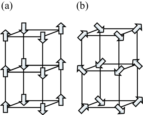
Figure 1: The spin configurations in the ground state. (a) Antiferromagnetically aligned ferromagnetic chains (af-FMC) order, and (b) one of the LT orders which have the continuous $O(3)$ symmetry.

In the present work we focus on a dipolar cube cut out from the SC dipolar lattice, with its edges being parallel to the lattice axes, and look for finite-size effects on its ground-state structures and its freezing characteristics by the stochastic molecular dynamics (MD) simulation. We have found very peculiar aspects which one cannot think of for finite-size systems with any short-range interaction. The ground state of the dipolar cube consists of 12 domains, each of which is very close to one of three af-FMC orders mentioned above. A very peculiar aspect we have observed in the cooling process is what we call from-edge-to-interior freezing characteristics: spins on the edges first freeze independently from spin freezing on other edges around the transition temperature of the corresponding bulk SC dipolar system, the af-FMC domains grow from the edges to the interior at lower temperatures, and then finally a unique combination of the domains is reached at the lowest temperature.

The model we study consists of classical Heisenberg spins, ${\vec{S}}$’s, which are arrayed on a finite cube. They correspond to magnetic moments of single ferromagnetic domain particles normalized by their magnetization $M_{\rm s}$. The dipole-dipole interaction energy between the spins is written as

$${\cal H}=\frac{J}{2a^{3}}\sum_{r_{ij}}{\vec{S}}_{i}\cdot\frac{1-{\vec{e}}_{ij}\otimes{\vec{e}}_{ij}}{r_{ij}^{3}}\cdot{\vec{S}}_{j}.$$ (1)

Here ${r}_{ij}$ denotes dimensionless length (normalized by the lattice constant, $a$) between sites $i$ and $j$, and ${\vec{e}}_{ij}$ the unit vector along the direction from site $i$ to site $j$. To the coupling constant, $J$, the value of $M_{s}^{2}$ is contained, and $J/a^{3}$ is put the energy (and temperature $T$ with $k_{\rm B}=1$) unit of the present model. For example, in Ni nanoparticles array with 30 nm particle diameter and $a\simeq 100$ nm,³⁾ $J/a^{3}$ is estimated about 5 K. If Co is replaced for Ni, $J/a^{3}$ becomes of order of several tens K. It is also worth quoting a typical value of magnetic molecular crystal, $J/a^{3}\simeq$ 0.7 K for $S_{z}$ = 10 with $a$ $\simeq$ 0.7 nm [11, 12].

The freezing characteristics of the model is analyzed by the Landau-Lifshiz-Gilbert (LLG) eq. [13],

$$\frac{d{\vec{S}_{i}}}{dt}=\frac{\gamma}{1+\alpha^{2}}{\vec{S}_{i}}\times\left\{{\vec{H}_{{\rm eff},i}}-\frac{\alpha}{M_{s}}{\vec{S}_{i}}\times{\vec{H}_{{\rm eff},i}}\right\},$$ (2)

with the effective magnetic field, ${\vec{H}_{{\rm eff},i}}$, given by

$${\vec{H}_{{\rm eff},i}}=\frac{\partial{\cal H}}{\partial\vec{S}_{i}}+{\vec{f}}_{i},$$ (3)

where ${\cal H}$ is the dipole-dipole interaction of Eq. (1). To include the heat-bath effect of temperature $T$ we introduce random force ${\vec{f}}_{i}$, its root mean square value being proportional to $T\alpha$. $\alpha$ and $\gamma$ are so-called Gilbert damping constant and the gyromagnetic constant, respectively. In the present study we solve the above set of equations based on the Euler method with conserving the norm of spins ($M_{s}=1$) and by setting $\alpha a^{3}/M_{s}\gamma J$ as the time unit. We further put both constants $\alpha$ and $\gamma$ to 1.0, and the time step of integrating Eq. (2), $\Delta t$, to 0.01. With this choice of the parameter values, the Larmor precession of a spin due to the internal field of averaged magnitude damps in a time comparable with one period of the precession at $T=0$.

In the present work we mainly report the results obtained by simulations on a cube whose linear size, $L$, is set to 16. It is an optimal size to look for peculiar phenomena in a magnetic dipolar cube: the size should be large enough to enable us to observe typical behavior of spins both on the boundary (corners, edges, and surfaces) and inside the cube, while simulation on a too large system is beyond computational power available for us. We note that, in the present simulation the sum in Eq. (1) are faithfully taken into account except for the analysis to obtain the result shown in Fig. 3(b) below.

We perform typically 8 cooling runs with a fixed cooling rate, in which we use different sets of random numbers generating their initial configurations as well as fluctuation forces. The average over them is carried out to obtain nearly-equilibrium, or frozen values of the observables reported below unless otherwise indicated. In each cooling run, temperature $T$ is initially set to 1 ($=J/a^{3}$) and is decreased by a step of $\Delta T=0.02$. At each temperature Eq. (2) is integrated by a period of $\tau=$ 5 $\times$ 10⁴$\Delta t$, which corresponds to about 500 periods of the Larmor precession mensioned above. The average value of quantities of our interest at each temperature is defined by that over the whole period of $\tau$. For example, the freezing of individual spins, ${\cal S}_{i}$, is evaluated as

$${\cal S}_{i}=\frac{1}{\tau}\left|\int_{\tau}\vec{S}_{i}(t)dt\right|.$$ (4)

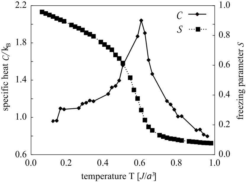
Figure 2: The specific heat ${\cal C}$ and the freezing parameter ${\cal S}$ as a function of temperature T.

Let us first present the results of global thermodynamic quantities. In Fig. 2, we demonstrate the specific heat, ${\cal C}$, and the overall freezing parameter, ${\cal S}$, as a function of temperature. Here ${\cal S}$ is defined as ${\cal S}=N^{-1}\sum_{i}{\cal S}_{i}$, including the average over the cooling runs, where $N$ is the total number of spins in the cube. It represents on average how much each spin is frozen in a time scale of $\tau$. We see from Fig. 2 that the specific heat exhibits a peak at $T^{*}\sim 0.6$, which is closed to the transition temperature, $T_{\rm c}=0.56$, evaluated previously in the corresponding bulk system [9]. Correspondingly, ${\cal S}$ starts to rapidly increase around $T^{*}$. Both ${\cal C}$ and ${\cal S}$ clearly indicate occurrence of cooperative freezing around $T^{*}$.

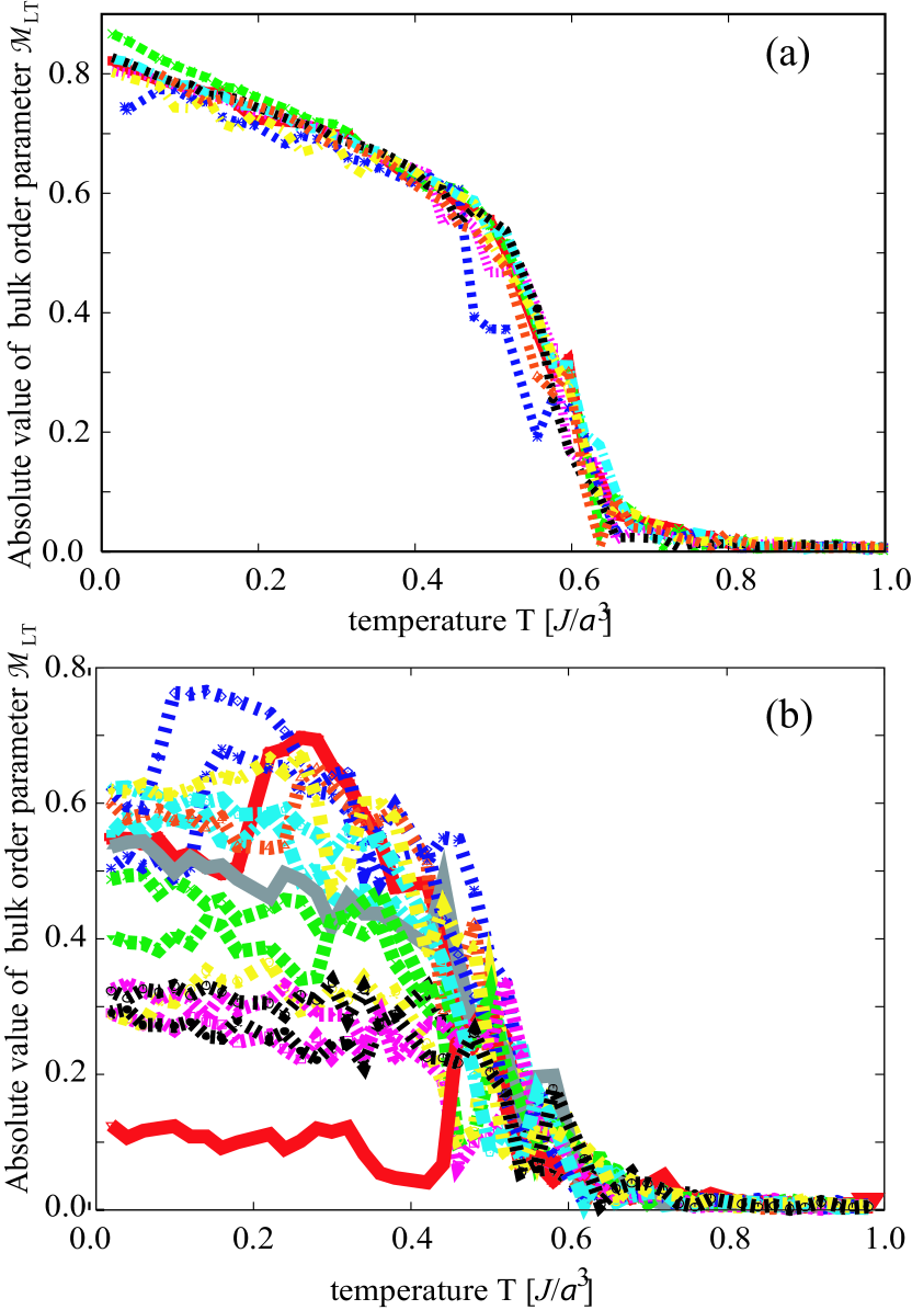
Figure 3: The LT order parameter ${\cal M}_{\rm LT}$ of the dipolar cube observed in 8 freezing runs; a) without and b) with cut-off for the dipole-dipole interaction.

It is natural for us to expect that the frozen order we found in the cube somehow reflects the magnetic structure of the bulk ground-state derived analytically by LT. The order parameter, which represents the LT ground-state order (see Fig. 1(a,b)), is defined by a vector, $\vec{\cal M}_{\rm LT}$, whose $\alpha$-component is written as

$${\cal M^{\alpha}}_{\rm LT}=\frac{1}{\tau}\int_{\tau}\sum_{i}(-1)^{\sum_{\beta\neq\alpha}n_{i}^{\beta}}S_{i}^{\alpha}(t)dt,$$ (5)

where $\alpha,\beta\in\{x,y,z\}$, and $n_{i}^{\alpha}$ denotes the $\alpha$-coordinate of site $i$. The absolute magnitudes of $\vec{\cal M}_{\rm LT}$, denoted as ${\cal M}_{\rm LT}$, for the 8 cooling runs are shown in Fig. 3(a). All ${\cal M}_{\rm LT}$’s start to rapidly increase from 0 around $T^{*}$ with decreasing temperature and reach almost a unique value of about 0.8 which is significantly less than the value of the bulk order, 1.0, at the lowest temperature. One plausible interpretation of the result is that spins on the cube reach a stable state which consists of the domains with different af-FMC orders. Figure 3(b), on the other hand, are ${\cal M}_{\rm LT}$’s obtained by the identical simulation as above but with one difference, namely, the dipole-dipole interaction is cut off within the range of $L/2$ in this simulation. By the introduction of the cut-off, the freezing behavior of ${\cal M}_{\rm LT}$ fluctuates drastically among 8 cooling runs, though ${\cal C}$ and ${\cal S}$ do not exhibit such a qualitative difference (not shown).

To check the above interpretation on the result shown in Fig. 3(a), we examine freezing patterns $\{{\cal S}_{i}\}$ defined by Eq. (4) of whole the cube. Figures 4(a-d) are typical result observed in one of the cooling processes. At $T=0.68\ (\geq T^{*})$, spins on some edges start to freeze. As the temperature further decreases ($T=0.6\leq T^{*}$), the freezing extends to the whole boundary in the sense that boundary spins are relatively less fluctuating than inner spins. This feature is kept at further lower temperatures. At $T=0.52$, however, spins in a domain indicated by the circle in Fig. 4(c) look as if they are partially melting. Finally at very low temperatures such as $T=0.36$, also inner spins almost freeze in the time scale of our observation. We can say that, in a cooling process of the present dipolar cube, spins on edges are the most stable, and those on boundary surfaces are stabler than those inside the cube.

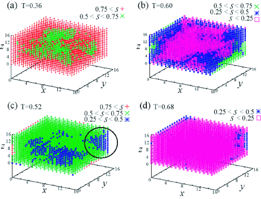
Figure 4: Patterns of $\{S_{i}\}$’s defined by eq. 4 for T=0.625, 0.5, 0.375 and 0.125.

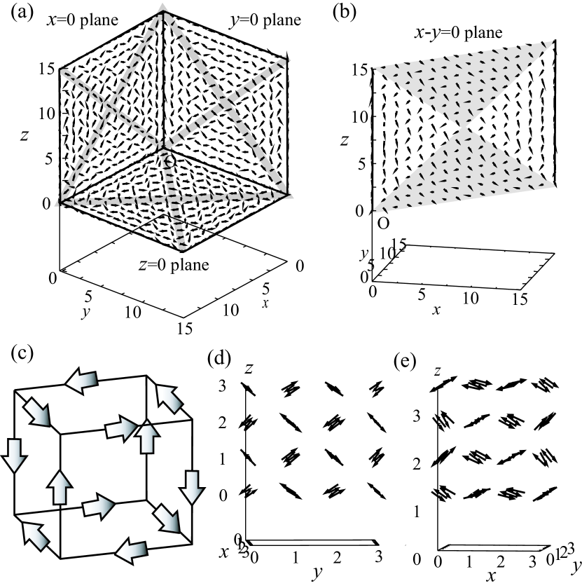
Figure 5: The spin configurations for the surfaces (a) and interior (b) of the dipolar cube at lowest temperatures. The shaded regions denote domain walls. Figure (c) represents the domain order in the ground state of the dipolar cube. Figures (d,e) are the spin configuration in the ground state of the $L$=4 dipolar cube.

A typical spin configuration at a very low temperature reached after the cooling process is shown in Figs. 5(a,b). A common property shared with such spin configurations is that spins on a boundary surface (including an edge) tend to align in the direction parallel to the surface (the edge). This tendency can be naively attributed to the anisotropic nature of the dipole-dipole interaction of Eq. (1). Namely, on a surface where there are two (one) axes parallel (perpendicular) to the surface, a ferromagnetic chain (FMC) aligned in parallel to the surface is more favorable. Naturally, on an edge an FMC order parallel to the edge is most favorable. Consequently, we can also expect that the magnetic structure at the lowest temperatures consists of 12 domains with short-range order which is close to one of the three af-FMC orders whose FMC order develops along the edge of each domain. This is in fact seen in Figs. 5(a,b). Also, if the simulation is started from one of the af-FMC configurations such as show in Fig. 1(a), it ends up with a similar configuration to the one shown in Figs. 5(a, b): the spins on a boundary initially in the direction perpendicular to the boundary flop into the parallel directions to the boundary.

By further inspection of the spin configurations, we find that the one with the lowest energy satisfies the following two conditions; the FMC orders on three edges which cross at each corner take 2-in(out)-1-out(in) configuration and those on opposite sides of a surface is aligned antiparallelly. These two conditions make the combination of domains in the ground state to be unique one which is shown in Fig 5(c). Here structures which can be connected by $\pi$/2-rotation around 4-fold axis of the cubic sample are regarded as identical. In this context, we want to emphasize that the proper self-rearrangement of the domains is due to the very long-range nature of the dipole-dipole interaction. In fact, when the cut-off of the interaction is introduced, each cooling run ends up with states with different values of ${\cal M}_{\rm LT}$ as indicated in Fig. 3(b), i.e., the adjustment of the af-FMC domains to reach their ground-state combination hardly takes place when the dipole-dipole interaction is cut off.

One more important freezing aspect we have observed is as follows. In the ground-state configuration, individual local energies of the corner spins are higher than those of other spins as expected. However, those of the edge spins are not necessarily lower than those of the interior spins. This implies that the relatively stronger freezing tendency discussed above can not be simply attributed to energetics of individual spins. Instead, we have to consider cooperative nature of the freezing. As noted above, the bulk LT order has the continuous $O(3)$ symmetry, and so different LT short-range orders are expected to grow in the bulk system, or inside the cube as well, at higher temperatures than $T_{\rm c}$ or $T^{*}\ (\simeq T_{\rm c})$. On the boundary of the cube, however, a symmetry breaking due to the presence of boundary partially solves the degeneracy. Especially on an edge, an FMC order along the edge direction, which has only the $Z_{2}$ symmetry as a whole, becomes preferable. This symmetry lowering of the short-range order is considered to be an origin of the from-edge-to-interior freezing characteristics we have found at and below $T^{*}$. Thus the boundary geometry, combined with the anisotropic nature of the dipole-dipole interaction, also plays an important role on the freezing nature of the dipolar cube.

So far the dipolar cube with $L=16$ has been discussed. For an odd-$L$ dipolar cube, one of the two conditions for the ground-state configuration for an even-$L$ cube mentioned above is certainly violated, since FMC’s on opposite sides of an odd-$L$ square in its ground state are checked to be parallel to each other.[15] We also note the stable configurations in cubes with small $L$’s. In the $L=16$ cube, spins around a vertex of the cube take an optimized direction, which is regarded as a part of the so-called vortex structures. [8] In small cubes with $L=4,6,8$, this corner structure extends to a size comparable with $L/2$, and consequently their ground state consists of a single-domain vortex state as shown in Fig. 3(d,e) which differs distinctly from the configuration shown in Figs. 5(a,b). We can expect variety of stable configurations of SC dipolar cubes arising from the relative angles between edges of the cube and the lattice axes. Further variety of magnetic properties of finite dipolar systems is expected when we think of the shape effect, different lattice structures, and so on. The present work has just opened a door in this interesting field.

To conclude let us summarize a scenario of the from-edge-to-interior freezing process we have found in the dipolar cube. 1) At higher temperatures than $T^{*}\ (\simeq T_{\rm c})$, the LT short-range orders are expected to grow. 2) Around $T^{*}$, where some of the LT short-range orders become in touch with one of the cube edges, the degeneracy in the LT orders is lifted, and one of the af-FMC orders fitted to the edge direction becomes stabilized. 3) The domains with the af-FMC order extends from edge to interior at lower temperatures. 4) In case the combination of domain structures does not match with the one of the ground-state, upturns of certain domains occur, and 5) the spin configuration reaches to the unique ground-state at lowest temperatures.

The present work is supported by NAREGI Nanoscience Project from the Ministry of Education, Culture, Sports, Science, and Technology. The numerical simulations have been partially performed also by using the facilities at the Supercomputer Center, Institute for Solid State Physics, the University of Tokyo.

References

- [1] S. Y. Chou, M. S. Wei, P. R. Krauss and P. B. Fischer, J. Appl. Phys. 76, 6673 (1994).
- [2] P. R. Arias, D. Altbir and M. Bahiana, cond-mat/0409374v1.
- [3] J. Füzi and L. K. Varga, Physica B 343, 320 (2004).
- [4] G. Szabó and G. Kádár, Phys. Rev. B 58, 5584 (1998).
- [5] J. F. Fernández, Phys. Rev. B 66, 064423 (2002).
- [6] J. A. Sauer, Phys. Rev. 57, 142 (1940).
- [7] J. M. Luttinger and L. Tisza, Phys. Rev. 70, 954 (1946).
- [8] P. I. Belobrov, R. S. Gekht and V. A. Ignatchenko, Zh. Eksp. Theo. Fiz. 84, 1097 (1983).
- [9] S. Romano, Nouvo Cimento D 7, 717 (1986).
- [10] Y. Tomita, K. Matsushita, A. Kuroda, R. Sugano, and H. Takayama, to appear in Computer Simulation Studies in Condensed Matter Physics XVIII, Eds. D. P. Landau, S. P. Lewis, and H.-B. Schüttler (Springer-Verlag, Heidelberg, Berlin).
- [11] J. R. Friedman, M. P. Sarachik, J. Tejada and R. Ziolo, Phys. Rev Lett. 76, 3830 (1996).
- [12] W. Wernsdorfer, T. Ohn, C. Sangregrio, R. Sessoli, D. Mailly and C. Paulsen, Phys. Rev. Lett. 82, 3903 (1999).
- [13] L. D. Landau and E. M. Lifshitz, Z. Phys. Sowjet. 8, 153 (1935).
- [14] J. L. GarcΓ́16a-Palacios and F. J. Lázaro, Phys. Rev. B 58, 14937 (1998).
- [15] R. Sugano et al., unpublished.