Interface mediated interactions between particles – a geometrical approach

Abstract

Particles bound to an interface interact because they deform its shape. The stresses that result are fully encoded in the geometry and described by a divergence-free surface stress tensor. This stress tensor can be used to express the force on a particle as a line integral along any conveniently chosen closed contour that surrounds the particle. The resulting expression is exact (i. e., free of any “smallness” assumptions) and independent of the chosen surface parametrization. Additional surface degrees of freedom, such as vector fields describing lipid tilt, are readily included in this formalism. As an illustration, we derive the exact force for several important surface Hamiltonians in various symmetric two-particle configurations in terms of the midplane geometry; its sign is evident in certain interesting limits. Specializing to the linear regime, where the shape can be analytically determined, these general expressions yield force-distance relations, several of which have originally been derived by using an energy based approach.

I Introduction

The interaction between spatially separated objects is mediated by the disturbance of the region that surrounds them, described by a field. In electromagnetic theory for example the interaction between charged particles is described by the Maxwell field equations. Since they are linear, interactions add. However, more often than not, the field equations are nonlinear as for example in the case of General Relativity: even though the energy-momentum tensor couples linearly to the curvature, the latter depends in a nonlinear way on the spacetime metric and its derivatives MTW ; Wald ; Weinberg . The source of the nonlinearity lies in the geometric nature of the problem. Not only do interactions fail to add up, even the humble two particle problem poses challenges.

“Effective” interactions between macroscopic degrees of freedom arise in statistical physics when a partial trace is performed in the partition function over unobserved microscopic degrees of freedom Belloni00 ; Likos01 . The Boltzmann factor invariably renders these interactions nonlinear. This time, the source of the nonlinearity is the entropy hidden in the degrees of freedom that have been traced out. For example, the effective interaction between charged colloids in salty water is described (at a mean-field level) by the Poisson-Boltzmann equation Hill .

In this paper we will discuss a classical example which belongs to the class of effective interactions, while owing its nonlinearity to its geometric origin: the interaction between particles mediated by the deformation of a surface to which they are bound. This problem includes the capillary interactions between particles bound to liquid-fluid interfaces pinningexp ; pinningtheo ; Kralchevsky , or the membrane mediated interactions between colloids or proteins adhering to or embedded in lipid bilayer membranes Kralchevsky ; Koltover ; Weiklcyl ; gbp ; inclusions ; Fourspher ; Kim ; BisBis . To approach the problem we require two pieces of information. First, how does the energy of the surface depend on its shape, or in other words, what is the “surface Hamiltonian”? Second, how does a bound particle locally deform the surface? With this information, we may (in principle) deduce the equilibrium shape minimizing the energy of the surface for any given placement of the bound particles. Knowing the shape, the energy can be determined by integration, and the forces it implies follow by differentiating with respect to appropriate placement variables. In general, however, the ground state of the surface is a solution of a nonlinear field equation (“the shape equation”), thereby thwarting progress by this route at a very early stage.

Sometimes the linearization of a nonlinear theory is adequate. Just as one recovers Newtonian gravitation as the weak-field limit of General Relativity MTW ; Wald ; Weinberg , or Debye-Hückel theory as the weak-field limit of Poisson-Boltzmann theory Hill , a linear theory for surface mediated interactions is useful for certain simple geometries, notably weakly perturbed flat surfaces. At this level, the approach to interactions based on energy becomes tractable. Yet, linearization is also often inadequate. The full theory may display qualitatively new effects which are absent in the linearized theory: strong gravitational fields give us black holes MTW ; Wald ; Weinberg ; the bare charge of a highly charged colloid gets strongly renormalized by counterion condensation colloidchargeren .

There is, however, an alternative approach to interactions which was outlined in mem_inter . By relating the interaction between particles to the equilibrium geometry of the surface, a host of exact nonlinear results is provided. The link is formed by the surface stress tensor, and it can be established without solving the shape equation. Once we know the Hamiltonian, we can express the stress at any point in terms of the local geometry – covariantly and without any approximation. We will briefly revisit the essentials of this construction in Sec. II. Knowing the stresses, the force on a particle is then determined by a line integral of the stress tensor along any surface contour enclosing the particle, as we will show in Sec. IV.

Such results might, at first sight, appear somewhat formal: without the equilibrium surface shape, they cannot be translated into hard numbers. However, the close link between the force and the geometry, combined with a very general knowledge one has about the surface shape (e. g., its symmetry) will turn out to provide valuable qualitative insight into the nature of the interaction (e. g., its sign). Even on a completely practical level, this approach scores points against the traditional approach involving energy, providing a significantly more efficient way to extract forces from the surface shape determined numerically (in whatever way).

We will illustrate this approach with a selection of examples involving different symmetries and surface Hamiltonians. In Sec. III we demonstrate how its scope extends in a very natural way to include internal degrees of freedom on the membrane – in particular: a vector order parameter which has for instance been used to describe lipid tilt HelPro88 ; MacLub ; NePo9293 ; SeShNe96 ; HamKoz00 ; tilt_force . To make contact with the energy based approach in the literature, and also in order to link the formalism to a more familiar setting, we specialize in Sec. V to a Monge parametrization and its linearization. This will permit us in Sec. VI to derive force-distance curves for interactions mediated by surface tension, membrane curvature, and lipid tilt. Various well-known linear results pinningexp ; pinningtheo ; Weiklcyl then follow very naturally using the stress tensor approach.

II Energy from Geometry

In this paper we want to study the physics of interfaces, which are characterized by a reparametrization invariant surface Hamiltonian. The appropriate language for this is differential geometry, and in this section we will outline how physical questions can be formulated very efficiently in this language. We first summarize the necessary mathematical basics and introduce our notation (the reader will find more background material in Refs. DifferentialGeometry ). We then define the class of Hamiltonians we will be considering. The corresponding Euler-Lagrange equations for the interface degrees of freedom will be cast as a conservation law. The most direct way to do this is to implement all geometrical constraints using Lagrange mulipliers; not only does this approach provide a quick derivation of the shape equation, it also provides a transparent physical identification of the surface stresses.

II.1 Differential Geometry and Notation

We consider a two-dimensional surface $\Sigma$ embedded in three-dimensional Euclidean space $\mathbb{R}^{3}$, which is described locally by its position ${\boldsymbol{X}}(\xi^{1},\xi^{2})\in\mathbb{R}^{3}$, where the $\xi^{a}$ are a suitable set of local coordinates on the surface. The embedding functions ${\boldsymbol{X}}$ induce two geometrical tensors which completely describe the surface: the metric $g_{ab}$ and the extrinsic curvature $K_{ab}$, defined by

$$g_{ab} = {\boldsymbol{e}}_{a}\cdot{\boldsymbol{e}}_{b}\qquad\text{and}$$ (1a)

$$K_{ab} = {\boldsymbol{e}}_{a}\cdot\partial_{b}{\boldsymbol{n}}\ ,$$ (1b)

where $a,b\in\{1,2\}$. The local coordinate frame formed by the tangent vectors ${\boldsymbol{e}}_{1}$ and ${\boldsymbol{e}}_{2}$ extended by the normal vector ${\boldsymbol{n}}$ forms a local basis of $\mathbb{R}^{3}$:

$${\boldsymbol{e}}_{a} = \partial{\boldsymbol{X}}/\partial\xi^{a}\;=\;\partial_{a}{\boldsymbol{X}}\ ,$$ (2a)

$${\boldsymbol{e}}_{a}\cdot{\boldsymbol{n}} = 0\ ,$$ (2b)

$${\boldsymbol{n}}^{2} = 1\ .$$ (2c)

Note that unlike ${\boldsymbol{n}}$, the ${\boldsymbol{e}}_{a}$ are generally not normalized.

In the following, $\nabla_{a}$ denotes the metric-compatible covariant derivative covariant_derivative and $\Delta=\nabla_{a}\nabla^{a}$ the corresponding Laplacian. Surface indices are raised with the inverse metric $g^{ab}$. The trace of the extrinsic curvature, $K=g^{ab}K_{ab}$, is twice the mean curvature. Using the above sign conventions, a sphere of radius $a$ with outward pointing unit normal has a positive $K=2/a$.

The intrinsic and extrinsic geometries are related by the Gauss-Codazzi-Mainardi equations

$$\nabla_{a}K_{bc}\,-\,\nabla_{b}K_{ac} = 0\ ,$$ (3a)

$$K_{ac}K_{bd}-K_{ad}K_{bc} = R_{abcd}\ ,$$ (3b)

where $R_{abcd}$ is the Riemann tensor constructed with the metric; its contraction over the first and third index is the Ricci tensor, $R_{bd}=g^{ac}R_{abcd}$, whose further contraction gives the Ricci scalar curvature, $R=g^{bd}R_{bd}$. From Eqn. (3b) we see that the latter satisfies $R=K^{2}-K^{ab}K_{ab}$. In particular in two dimensions we have that $R=2\,K_{\text{G}}$, where $K_{\text{G}}=\det(K_{a}^{b})$ is the Gaussian curvature (Gauss’ Theorema Egregium DifferentialGeometry ).

II.2 Surface energy and its variation

We consider surfaces such as lipid membranes and soap films, characterized by the property that the associated energy is completely determined by the surface geometry and described by a Hamiltonian which is an integral of a local Hamiltonian density $\mathcal{H}$ over the surface:

$$H[{\boldsymbol{X}}]=\int_{\Sigma}{\operatorname{d}}A\;\mathcal{H}(g_{ab},K_{ab},\nabla_{a}K_{bc},\ldots)\ .$$ (4)

The infinitesimal area element is ${\operatorname{d}}A=\sqrt{g}\,{\operatorname{d}}^{2}\xi$, where $g=\det(g_{ab})$ is the determinant of the metric. The density $\mathcal{H}$ depends only on scalars constructed from local surface tensors: the metric, the extrinsic curvature, and its covariant derivatives. In order to find the equilibrium (i. e., energy minimizing) shape, one is interested in how $H$ responds to a deformation of the surface described by a change in the embedding functions, ${\boldsymbol{X}}\rightarrow{\boldsymbol{X}}+\delta{\boldsymbol{X}}$. The straightforward (but tedious) way to do this is to track the course of the deformation on ${\boldsymbol{X}}$ through $g_{ab}$, $\sqrt{g}$, $K_{ab}$, and any appearing covariant derivatives using the structural relationships (1) and (2).

Alternatively, one can treat $g_{ab}$, $K_{ab}$, ${\boldsymbol{e}}_{a}$ and ${\boldsymbol{n}}$ as independent variables, enforcing the structural relations (1) and (2) using Lagrange multiplier functions Guven04 . One thus introduces the new functional $H_{\text{c}}[g_{ab},K_{ab},\ldots,{\boldsymbol{X}},{\boldsymbol{e}}_{a},{\boldsymbol{n}},\lambda^{ab},\Lambda^{ab},{\boldsymbol{f}}^{a},\lambda_{\perp}^{a},\lambda_{n}]$ given by

$$H_{\text{c}} = H[g_{ab},K_{ab},\ldots]$$ (5)

$$\stackrel{{\scriptstyle\text{(\ref{eq:gab})}}}{{+}}\int{\operatorname{d}}A\;\lambda^{ab}(g_{ab}-{\boldsymbol{e}}_{a}\cdot{\boldsymbol{e}}_{b})$$

$$\stackrel{{\scriptstyle\text{(\ref{eq:Kab})}}}{{+}}\int{\operatorname{d}}A\;\Lambda^{ab}(K_{ab}-{\boldsymbol{e}}_{a}\cdot\partial_{b}{\boldsymbol{n}})$$

$$\stackrel{{\scriptstyle\text{(\ref{eq:ea})}}}{{+}}\int{\operatorname{d}}A\;{\boldsymbol{f}}^{a}\cdot({\boldsymbol{e}}_{a}-\partial_{a}{\boldsymbol{X}})$$

$$\stackrel{{\scriptstyle\text{(\ref{eq:ea_normal_n})}}}{{+}}\int{\operatorname{d}}A\;\lambda_{\perp}^{a}({\boldsymbol{e}}_{a}\cdot{\boldsymbol{n}})$$

$$\stackrel{{\scriptstyle\text{(\ref{eq:n2=1})}}}{{+}}\int{\operatorname{d}}A\;\lambda_{n}({\boldsymbol{n}}^{2}-1)\ .$$

The original Hamiltonian $H$ is now treated as a function of the independent variables $g_{ab}$, $K_{ab}$ and its covariant derivatives; $\lambda^{ab}$, $\Lambda^{ab}$, ${\boldsymbol{f}}^{a}$, $\lambda_{\perp}^{a}$ and $\lambda_{n}$ are Lagrange multipliers fixing the constraints (1) and (2). The introduction of auxiliary variables greatly simplifies the variational problem, because now we do not have to track explicitly how the deformation $\delta{\boldsymbol{X}}$ propagates through to $g_{ab}$ and $K_{ab}$. As we will see in the following, this approach also provides a very simple and direct derivation of the shape equation in which the multiplier ${\boldsymbol{f}}^{a}$, which pins the tangent vectors to the surface, is identified as the surface stress tensor.

Note that additional physical constraints can be enforced by introducing further Lagrange multipliers (such as a pressure $P$ in the case that a fixed volume is enclosed by the surface).

II.3 Euler-Lagrange equations and the existence of a conserved current

The Hamiltonian (4) is invariant under translations. As explained in detail in Ref. surfacestresstensor , Noether’s theorem then guarantees the existence of an associated conserved current, which we will identify as the surface stress tensor in Sec. II.4. In order to see this, let us first work out the Euler-Lagrange equations for ${\boldsymbol{X}}$, ${\boldsymbol{e}}_{a}$, ${\boldsymbol{n}}$, $g_{ab}$ and $K_{ab}$:

$$\nabla_{a}{\boldsymbol{f}}^{a} = 0\ ,$$ (6a)

$${\boldsymbol{f}}^{a} = (\Lambda^{ac}K_{c}^{b}+2\lambda^{ab}){\boldsymbol{e}}_{b}-\lambda_{\perp}^{a}{\boldsymbol{n}}\ ,$$ (6b)

$$0 = (\nabla_{b}\Lambda^{ab}+\lambda_{\perp}^{a}){\boldsymbol{e}}_{a}+(2\lambda_{n}-\Lambda^{ab}K_{ab}){\boldsymbol{n}}\ ,$$ (6c)

$$\lambda^{ab} = \textstyle\frac{1}{2}\,T^{ab}\ ,$$ (6d)

$$\Lambda^{ab} = -\mathcal{H}^{ab}\ .$$ (6e)

Note that the Weingarten equations $\partial_{a}{\boldsymbol{n}}=K_{a}^{b}{\boldsymbol{e}}_{b}$ have been used in Eqn. (6b); the Gauss equations $\nabla_{a}{\boldsymbol{e}}_{b}=-K_{ab}{\boldsymbol{n}}$ have been used in Eqn. (6c). We have also defined

$$\mathcal{H}^{ab} = \frac{\delta\mathcal{H}}{\delta K_{ab}}\qquad\text{and}$$ (7a)

$$T^{ab} = -\frac{2}{\sqrt{g}}\frac{\delta(\sqrt{g}\mathcal{H})}{\delta g_{ab}}\ .$$ (7b)

The manifestly symmetric tensor $T^{ab}$ is the intrinsic stress tensor associated with the metric $g_{ab}$. If $\mathcal{H}$ does not depend on derivatives of $K_{ab}$, functional derivatives in the definition of $\mathcal{H}^{ab}$ and $T^{ab}$ reduce to ordinary ones.

Equation (6a) reveals the existence of a conservation law for the current ${\boldsymbol{f}}^{a}$. Using the other equations (6c), (6d) and (6e), it is straightforward to eliminate the Lagrange multipliers on the right hand side of Eqn. (6b) to obtain an explicit expression for ${\boldsymbol{f}}^{a}$ in terms of the original geometrical variables. From Eqn. (6c) we find $\lambda_{\perp}^{a}=-\nabla_{b}\Lambda^{ab}$ because ${\boldsymbol{e}}_{a}$ and ${\boldsymbol{n}}$ are linearly independent; the Eqns. (6d) and (6e) determine $\lambda^{ab}$ and $\Lambda^{ab}$. Thus Eqn. (6b) can be recast as

$${\boldsymbol{f}}^{a}=(T^{ab}-\mathcal{H}^{ac}K_{c}^{b}){\boldsymbol{e}}_{b}-(\nabla_{b}\mathcal{H}^{ab}){\boldsymbol{n}}\ .$$ (8)

Once the Hamiltonian density has been specified, Eqn. (8) determines the conserved current ${\boldsymbol{f}}^{a}$ completely in terms of the geometry. Several representative examples are treated in the Appendix.

Finally, as pointed out in Refs. surfacestresstensor ; Guven04 , the normal projection of $\nabla_{a}{\boldsymbol{f}}^{a}$ is the Euler-Lagrange derivative $\mathcal{E}(\mathcal{H})$ of the original Hamiltonian $H$ which vanishes for an equilibrium shape E(H)=P . Using the Gauss equations once more, we obtain the remarkably succinct result

$${\boldsymbol{n}}\cdot\nabla_{a}{\boldsymbol{f}}^{a}=\mathcal{E}(\mathcal{H})=-K_{ab}T^{ab}+(K_{ac}K_{b}^{c}-\nabla_{a}\nabla_{b})\mathcal{H}^{ab}\ .$$ (9)

II.4 Identification of the stress tensor

We will now show that ${\boldsymbol{f}}^{a}$ can be identified with the surface stress tensor. The variation of the Hamiltonian has a bulk part proportional to the Euler-Lagrange derivative (6) as well as boundary terms: under a change in the embedding functions ${\boldsymbol{X}}\to{\boldsymbol{X}}+\delta{\boldsymbol{X}}$ one gets

$$\delta H_{\text{c}}=\int{\operatorname{d}}A\;\big{[}\nabla_{a}{\boldsymbol{f}}^{a}\cdot\delta{\boldsymbol{X}}-\nabla_{a}({\boldsymbol{f}}^{a}\cdot\delta{\boldsymbol{X}})\big{]}\ .$$ (10)

Additional boundary contributions stem from the variations with respect to ${\boldsymbol{n}}$, $g_{ab}$ and $K_{ab}$, since these terms do or may contain further derivatives which then need to be removed by partial integration. However, the one appearing in Eqn. (10) is the only one that is relevant for identifying the stress tensor: As we will see below, for this we are exclusively interested in translations, for which ${\boldsymbol{n}}$, $g_{ab}$ and $K_{ab}$ remain unchanged.

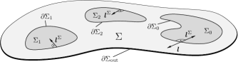
Figure 1: Surface $\Sigma$ with 3 disjoint boundary components $\partial\Sigma_{i}$ and an outer limiting boundary $\partial\Sigma_{\text{out}}$.

Consider, in particular, a surface region $\Sigma$ in equilibrium (see Fig. 1): its boundary $\partial\Sigma$ consists of $n$ disjoint closed components $\partial\Sigma_{i}$ and an outer limiting boundary $\partial\Sigma_{\text{out}}$. Each of the $\partial\Sigma_{i}$ is also the closed boundary of a surface patch $\Sigma_{i}$. Under a constant translation $\delta{\boldsymbol{X}}={\boldsymbol{a}}$ of $\partial\Sigma_{i}$ the only non-zero term is

$$\delta H_{\text{c}}=-{\boldsymbol{a}}\cdot\oint_{\partial\Sigma_{i}}{\operatorname{d}}s\;l^{\Sigma}_{a}{\boldsymbol{f}}^{a}=-{\boldsymbol{a}}\cdot{\boldsymbol{F}}^{(i)}_{\rm ext}\ .$$ (11)

Stokes’ theorem has been used to convert the surface integral into a line integral. The vector ${\boldsymbol{l}}^{\Sigma}=l^{\Sigma}_{a}{\boldsymbol{e}}^{a}$ is the outward pointing unit normal to the boundary on the surface $\Sigma$; by construction it is tangential to $\Sigma$. The variable $s$ measures the arc-length along $\partial\Sigma_{i}$. The boundary integral is thus identified as the external force ${\boldsymbol{F}}^{(i)}_{\rm ext}$ acting on $\partial\Sigma_{i}$: dotted into any infinitesimal translation, it yields (minus) the corresponding change in energy force_at_infinity .

The external force ${\boldsymbol{F}}_{\rm ext}$ on the surface patch $\Sigma_{0}$ is simply given by $-{\boldsymbol{F}}^{(0)}_{\rm ext}$ due to Newton’s third law

$${\boldsymbol{F}}_{\rm ext}=\oint_{\partial\Sigma_{0}}{\operatorname{d}}s\;l_{a}{\boldsymbol{f}}^{a}=\int_{\Sigma_{0}}{\operatorname{d}}A\;\nabla_{a}{\boldsymbol{f}}^{a}\;,$$ (12)

where ${\boldsymbol{l}}=-{\boldsymbol{l}}^{\Sigma}$ and Stokes’ theorem was used again.

Recall now that in classical elasticity theory LaLi_elast the divergence of the stress tensor at any point in a strained material equals the external force density. Or equivalently, the stress tensor contracted with the normal vector of a local fictitious area element yields the force per unit area transmitted through this area element. Comparing this with Eqn. (12) we see that ${\boldsymbol{f}}^{a}$ is indeed the surface analog of the stress tensor: $l_{a}{\boldsymbol{f}}^{a}$ is the force per unit length acting on the boundary curve due to the action of surface stresses.

It proves instructive to look at the tangential and normal projection of the stress tensor by defining

$${\boldsymbol{f}}^{a}=f^{ab}{\boldsymbol{e}}_{b}+f^{a}{\boldsymbol{n}}\ .$$ (13)

Using the equations of Gauss and Weingarten GaussWeingarten , the relation $\nabla_{a}{\boldsymbol{f}}^{a}=\mathcal{E}{\boldsymbol{n}}$ can then be cast in the form

$$\nabla_{a}f^{a} = K_{ab}f^{ab}+\mathcal{E}\ ,$$ (14a)

$$\nabla_{a}f^{ab} = -K_{a}^{b}f^{a}\ .$$ (14b)

Tangential stress acts as a source of normal stress – and vice versa. Both conditions hold irrespective of whether the Euler-Lagrange derivative $\mathcal{E}$ actually vanishes. In fact, Eqn. (14a) shows that the shape equation $\mathcal{E}=0$ is equivalent to $\nabla_{a}f^{a}=K_{ab}f^{ab}$, while Eqn. (14b) merely provides consistency conditions on the stress components. For instance, the Helfrich Hamiltonian $\mathcal{H}\propto K^{2}$ yields $f^{a}\propto\nabla^{a}K$, while $f^{ab}$ is a quadratic in the extrinsic curvature tensor (see Eqn. (86)). Hence, Eqn. (14a) immediately reproduces the characteristic form of the Euler-Lagrange derivative: $\Delta K$ plus a cubic in the extrinsic curvature.

III Internal degrees of freedom

So far we have restricted the discussion to Hamiltonians which are exclusively constructed from the geometry of the underlying surface. However, the surface itself may possess internal degrees of freedom which can couple to each other and, more interestingly, also to the geometry. The simplest example would be a scalar field $\phi$ on the membrane, which could describe a local variation in surface tension or lipid composition, and it is readily incorporated into the present formalism CaGu04 .

Here we will look a little more closely at the case of an additional tangential surface vector field $m^{a}$. Such a field has been introduced to describe the tilt degrees of freedom of the molecules within a lipid bilayer, to accommodate the fact that the average orientation of the lipids themselves need not coincide with the local bilayer normal (see for instance Refs. HelPro88 ; MacLub ; NePo9293 ; SeShNe96 ; HamKoz00 ; tilt_force ). Many additional terms for the energy emerge in the presence of a new field $m^{a}$ (for a systematic classification see Ref. NePo9293 ). However our aim here is not to treat the most general case. Instead, we will focus on a simple representative example to illustrate how easily the present formalism generalizes to treat such situations.

Let us define the properly symmetrized covariant tilt-strain tensors $M^{ab}$ and $F^{ab}$ according to

$$M^{ab} = \frac{1}{2}\big{(}\nabla^{a}m^{b}+\nabla^{b}m^{a}\big{)}\ ,$$ (15a)

$$F^{ab} = \;\;\;\;\;\nabla^{a}m^{b}-\nabla^{b}m^{a}\ .$$ (15b)

In the spirit of a harmonic theory we construct a Hamiltonian density $\mathcal{H}_{\operatorname{m}}$ from the following quadratic invariants:

$$\mathcal{H}_{\operatorname{m}}=\frac{1}{2}\lambda M^{2}+\mu M_{ab}M^{ab}+\frac{1}{4}\nu F_{ab}F^{ab}+V(m^{2})\ ,$$ (16)

where $M=g_{ab}M^{ab}=\nabla_{a}m^{a}$ is the tilt divergence. The first two terms coincide with the lowest order intrinsic terms identified by Nelson and Powers NePo9293 , provided we restrict to unit vectors $m^{a}$ unit_vectors . These terms are multiplied by new elastic constants $\lambda$ and $\mu$, playing the analogous role to Lamé-coefficients Lame . If $m^{2}\neq 1$ a third term (also absent in usual elasticity theory LaLi_elast ) occurs, the quadratic scalar constructed from the antisymmetrized tilt gradient; its structure is completely analogous to the Lagrangian in electromagnetism LaLi_electro . Finally, if the magnitude of $m^{a}$ is not fixed, we may also add a potential $V$ depending on the square $m^{2}=m_{a}m^{a}$ of the vector field $m^{a}$. Without loss of generality we assume that $V(0)=0$, because any nonvanishing constant is more appropriately absorbed into the surface tension $\sigma$. If $V(x)$ is minimal for $x=0$, then $m^{a}\equiv 0$ will minimize the energy, but depending on physical conditions $V$ may favor nonzero values of $|m^{a}|$. This is why below the main phase transition temperature of lipid bilayers the lipids can acquire a spontaneous tilt.

This particular choice for $\mathcal{H}_{\operatorname{m}}$ is purely intrinsic. Hence, Eqn. (8) shows that the corresponding material stress ${\boldsymbol{f}}_{\operatorname{m}}^{a}$ is also purely intrinsic, therefore tangential, and given by ${\boldsymbol{f}}_{\operatorname{m}}^{a}=T^{ab}_{\operatorname{m}}{\boldsymbol{e}}_{b}$, where $T^{ab}_{\operatorname{m}}=-2\sqrt{g}^{-1}\delta(\sqrt{g}\mathcal{H}_{\operatorname{m}})/\delta g_{ab}$ is the metric material stress. Performing the functional variation (see Appendix) we find

$$T^{ab}_{\operatorname{m}} = \frac{1}{2}\Big{[}\lambda\big{(}M^{2}+2m^{c}\nabla_{c}M\big{)}+\nu\big{(}\varepsilon_{cd}\nabla^{c}m^{d}\big{)}^{2}\Big{]}g^{ab}$$ (17)

$$+\,\mu\Big{[}-M_{cd}M^{cd}g^{ab}+2MM^{ab}+2m^{c}\nabla_{c}M^{ab}$$

$$\qquad\,-\,(\nabla_{c}m^{a})(\nabla^{c}m^{b})+(\nabla^{a}m_{c})(\nabla^{b}m^{c})\Big{]}$$

$$-\,V(m^{2})g^{ab}-2V^{\prime}(m^{2})m^{a}m^{b}\ ,$$

where $\varepsilon_{ab}={\boldsymbol{n}}\cdot({\boldsymbol{e}}_{a}\times{\boldsymbol{e}}_{b})$ is the antisymmetric epsilon-tensor epsilon_tensor . Notice that the metric stress tensor is quadratic in the tilt-strain, not linear. Unlike the stress tensor in elasticity theory, this tensor is not obtained as the derivative of the energy with respect to the strain but rather with respect to the metric, which leaves it quadratic in the strain. The formal analogy alluded to earlier is therefore not complete.

Adding the material stress $T^{ab}_{\operatorname{m}}$ to the tangential geometric stress $f^{ab}$, we find with the help of Eqns. (14) the equilibrium conditions

$$0 = -K_{ab}T^{ab}_{\operatorname{m}}+\mathcal{E}\ ,$$ (18a)

$$\nabla_{a}T^{ab}_{\operatorname{m}} = 0\ .$$ (18b)

The first of these equations shows how the material degrees of freedom “add” to the geometric Euler-Lagrange derivative $\mathcal{E}$ of the geometric Hamiltonian $\mathcal{H}$; this is the modified shape equation. The second equation – which before provided consistency conditions on the geometrical stresses – tells us that the material stress tensor is conserved. The equilibrium of the material degrees of freedom involves the vanishing of the Euler-Lagrange derivative with respect to the field $m^{a}$, which is given by

$$\mathcal{E}_{{\operatorname{m}}\,a}\;=\;\frac{\delta H_{\operatorname{m}}}{\delta m^{a}} = -\lambda\nabla_{a}\nabla_{b}m^{b}-(\mu+\nu)\nabla_{b}\nabla_{a}m^{b}$$ (19)

$$-\;(\mu-\nu)\Delta m_{a}+2V^{\prime}(m^{2})m_{a}\ .\;\;\;$$

In general, the equilibrium condition $\mathcal{E}_{{\operatorname{m}}\,a}\equiv 0$ implies Eqn. (18b). For a single vector field $m^{a}$ the converse also holds so that Eqn. (18b) may be used in place of the equilibrium condition equiv .

In equilibrium, we have not only $\mathcal{E}_{{\operatorname{m}}\,a}\equiv 0$, we also have $\nabla^{a}\mathcal{E}_{{\operatorname{m}}\,a}=0$. Using the commutation relations for covariant derivatives commutation , it is then easy to see that the tilt also satisfies the following equation on the surface:

$$(\lambda+2\mu)\Delta M+\mu\nabla^{a}(Rm_{a})-2\big{[}2V^{\prime\prime}m^{2}+V^{\prime}M\big{]}\;=\;0\ .$$ (20)

Notice that $\nu$ has dropped out of this equation, which follows from the fact that $F^{ab}$ is invariant under $U(1)$ gauge transformations gauge . For small values of tilt, we can expand the potential as

$$V(m^{2})=\frac{1}{2}tm^{2}+\frac{1}{4}um^{4}+\cdots$$ (21)

In the untilted phase we can terminate this expression after the first term (since then $t>0$). If we now restrict to a flat membrane (and thus $R\equiv 0$) Eqn. (20) simplifies to a Helmholtz equation for the tilt divergence:

$$\big{[}(\lambda+2\mu)\Delta-t\big{]}\,M\;=\;0\ ,$$ (22)

showing that (in lowest order) any nonzero $M$ is (essentially) exponentially damped with a decay length of

$$\ell_{\operatorname{m}}=\sqrt{\frac{\lambda+2\mu}{t}}\ .$$ (23)

If $t<0$ gets us into the tilted phase, the expansion (21) has to be taken one order higher, leaving instead a nonlinear Ginzburg-Landau equation to be solved.

We finally remark that even though the system of Euler-Lagrange equations (18) is quite formidable, it still enjoys one nice nontrivial property: The material equation (18b) is purely intrinsic. This is the case because the material stress is tangential, which itself derives from the fact that the material Hamiltonian is intrinsic. If we were to add a coupling between tilt and extrinsic curvature, such as the chiral term $\varepsilon_{ac}K^{c}_{b}m^{a}m^{b}$, this decoupling would no longer hold.

IV Forces between particles

Particles bound to an interface can exert indirect forces onto each other. Since these are mediated by the interface, they must be encoded in its geometry. We have seen that the “coding” is done by the surface stress tensor ${\boldsymbol{f}}^{a}$. The problem is to decode this content.

In this section we will solve this problem. The strong link between stress and geometry can be easily turned into exact expressions for mediated interactions. The method by which we obtain these results for various different Hamiltonians as well as the final formulas are one of the major results of this paper.

IV.1 The stress tensor and external forces

Consider a single simply-connected patch $\Sigma_{0}$. The external force acting on it is given by Eqn. (12). If there are no external external forces acting on $\Sigma_{0}$, the integrals appearing in Eqn. (12) will vanish; but even when ${\boldsymbol{F}}_{\rm ext}$ does not vanish, the stress tensor remains divergence free (Eqn. (6a)) on any part of the surface not externally acted upon. As a result, the contour integral appearing in Eqn. (12) will be independent of the particular closed curve so long as it continues to enclose the source of stress and does not encroach on any other sources.

Observe now that in general a multi-particle configuration can be stationary only if external forces constrain the particle positions. These are the forces providing the source of stress in Eqn. (12). The force ${\boldsymbol{F}}$ we are ultimately interested in is the force on a particle mediated by the interface counteracting this external force; we therefore evidently have ${\boldsymbol{F}}=-{\boldsymbol{F}}_{\rm ext}$.

IV.2 Force between particles on a fluid membrane

Let us now focus on a symmetric fluid membrane, described by the surface Hamiltonian

$$\mathcal{H}=\frac{1}{2}\kappa\,K^{2}+\sigma\ ,$$ (24)

which, up to irrelevant boundary terms, is equivalent to the Hamiltonians introduced by Canham Canham and Helfrich Helfrich . Here, $\kappa$ is the bending rigidity and $\sigma$ is the lateral tension imposed on the boundary. For typical phospholipid membranes $\kappa$ is of the order of a few tens of $k_{\text{B}}T$, where $k_{\text{B}}T$ is the thermal energy. Values for $\sigma$ are found to be in a broad range between 0 up to about 10 mN/m surfacetension . The Hamiltonian (24) covers interesting special cases in various limits: soap films on setting $\kappa=0$ and tensionless membranes on setting $\sigma=0$. Note that the two elastic constants provide a characteristic length

$$\ell:=\sqrt{\frac{\kappa}{\sigma}}\ ,$$ (25)

separating short length scales over which bending energy dominates from the large ones over which tension does.

We now need to determine the force (12) on a particle for the Hamiltonian described by Eqn. (24). Using Eqns. (85) and (86) from the Appendix, we obtain

$${\boldsymbol{f}}^{a}=\Big{[}\kappa\big{(}K^{ab}-\frac{1}{2}Kg^{ab}\big{)}K-\sigma g^{ab}\Big{]}\,{\boldsymbol{e}}_{b}-\kappa(\nabla^{a}K)\,{\boldsymbol{n}}$$ (26)

for the surface stress tensor associated with this Hamiltonian. To facilitate the calculation of the force it is convenient to introduce an orthonormal basis of tangent vectors $\{{\boldsymbol{t}},{\boldsymbol{l}}\}$ adapted to the contour $\partial\Sigma_{0}$: ${\boldsymbol{t}}=t^{a}{\boldsymbol{e}}_{a}$ points along the integration contour and, as introduced previously, ${\boldsymbol{l}}=l^{a}{\boldsymbol{e}}_{a}$ points normally outward. The elements of the extrinsic curvature tensor with respect to this basis are given by

$$K_{\perp} = l^{a}l^{b}K_{ab}\ ,$$ (27a)

$$K_{\|} = t^{a}t^{b}K_{ab}\ ,$$ (27b)

$$K_{\perp\|} = l^{a}t^{b}K_{ab}\ .$$ (27c)

We obtain for the integrand appearing in the line integral in Eqn. (12),

$$l_{a}{\boldsymbol{f}}^{a}=\Big{[}\kappa\big{(}l_{a}K^{ab}-\frac{1}{2}Kl^{b}\big{)}K-\sigma l^{b}\Big{]}\,{\boldsymbol{e}}_{b}-\kappa(\nabla_{\perp}K)\,{\boldsymbol{n}}\ ,$$ (28)

where we have defined the normal derivative $\nabla_{\perp}=l_{a}\nabla^{a}$. The first term can be simplified by exploiting the completeness of the tangent basis, $g_{b}^{c}=l_{b}l^{c}+t_{b}t^{c}$:

$$l_{a}K^{ab}{\boldsymbol{e}}_{b} = l_{a}K^{ab}(l_{b}l^{c}+t_{b}t^{c}){\boldsymbol{e}}_{c}$$ (29)

$$= l_{a}l_{b}K^{ab}{\boldsymbol{l}}+l_{a}t_{b}K^{ab}{\boldsymbol{t}}$$

$$= K_{\perp}{\boldsymbol{l}}+K_{\perp\|}{\boldsymbol{t}}\ .$$

Since furthermore the trace $K=K_{\perp}+K_{\|}$, we find

$${\boldsymbol{F}} = -\oint_{\partial\Sigma_{0}}\!\!\!{\operatorname{d}}s\;\bigg{\{}\Big{[}\frac{1}{2}\kappa\big{(}K_{\perp}^{2}-K_{\|}^{2}\big{)}-\sigma\Big{]}{\boldsymbol{l}}$$ (30)

$$\qquad\qquad+\;\kappa K_{\perp\|}K{\boldsymbol{t}}-\kappa\big{(}\nabla_{\perp}K\big{)}{\boldsymbol{n}}\bigg{\}}\ .$$

Note that the integrand has been decomposed with respect to a (right-handed) orthonormal basis adapted to the contour, $\{{\boldsymbol{l}},{\boldsymbol{t}},{\boldsymbol{n}}\}$.

IV.3 Two-particle configurations

We are interested in applying the general considerations of Sec. IV.1 to surface mediated interactions between colloidal particles. In particular, we will consider a symmetrical configuration consisting of two identical particles bound to an asymptotically flat surface, as sketched schematically in Fig. 2.

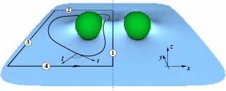
Figure 2: Two identical particles bound to an interface. As described in the text, the contour of integration can be deformed in order to take advantage of available symmetries.

We label by $\{{\boldsymbol{x}},{\boldsymbol{y}},{\boldsymbol{z}}\}$ the Cartesian basis vectors of three-dimensional Euclidian space $\mathbb{R}^{3}$. Remote from the particles, the surface is parallel to the $(x,y)$ plane.

Let us agree that the constraining force fixes only the separation between the particles; their height, as well as their orientation with respect to the $(x,y)$ plane are free to adjust and thus to equilibrate. This is also true of the contact line between surface and colloid when it is not pinned. Indeed, Kim et al. Kim carefully argue that vertical forces and horizontal torques typically exceed horizontal forces and vertical torques by a significant amount. Since the former can thus be assumed to very quickly equilibrate, they generally do not contribute to the membrane mediated interaction.

There are two distinct manifestations of two-particle symmetry in this situation: either a mirror symmetry in the $(y,z)$ plane (the symmetric case) or a twofold symmetry axis, coinciding with the $y$ axis (the antisymmetric case). The former is relevant if the two particles adhere to the same side of the surface, the latter applies if they adhere on opposite sides (see Fig. 3). In these two geometries the line joining corresponding points on the two particles lies along the $x$-direction.

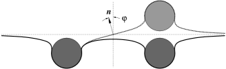
Figure 3: Cross-section of a symmetric (solid line) and an antisymmetric (dotted line) two-particle geometry.

It is now possible to deform the contour of the line integral (12) to our advantage: as indicated in Fig. 2, the contour describing the force on the left hand particle may always be pulled open so that the surface is flat on three of its four branches (2, 3 and 4). The contributions from branch 2 will cancel that from 4; the only mathematically involved term stems from branch 1. The force on the particle is then given by

$${\boldsymbol{F}}=-\bigg{[}\int_{1}+\int_{3}\bigg{]}{\operatorname{d}}s\;l_{a}{\boldsymbol{f}}^{a}\ .$$ (31)

Let us now apply this general approach to a surface whose energetics can be described by the Hamiltonian density (24).

IV.4 The force between particles with symmetry

IV.4.1 Fluid membranes

Both mirror and two-fold axial symmetry of branch 1 imply that in Eqn. (30) the tangential term proportional to ${\boldsymbol{t}}$ vanishes. In the first case this follows from the fact that branch 1 becomes a line of curvature; hence, the curvature tensor is diagonal in $({\boldsymbol{l}},{\boldsymbol{t}})$-coordinates and thus $K_{\perp\|}$ vanishes. In the second case two-fold axial symmetry forces both $K_{\|}$ as well as $K_{\perp}$ to be zero, since branch 1 becomes a straight line and the profile is antisymmetric. In consequence, $K=K_{\perp}+K_{\|}=0$. We thereby obtain the first important simplification of the force from Eqn. (30) on that branch:

$${\boldsymbol{F}}_{1}=-\int_{1}{\operatorname{d}}s\;\bigg{\{}\Big{[}\frac{1}{2}\kappa\big{(}K_{\perp}^{2}-K_{\|}^{2}\big{)}-\sigma\Big{]}{\boldsymbol{l}}-\kappa\big{(}\nabla_{\perp}K\big{)}{\boldsymbol{n}}\bigg{\}}\ .$$ (32)

We now examine separately the two symmetric geometries (see discussion in Sec. IV.3).

a. Symmetric case. Tangent and normal vector on branch 1 lie in the $(y,z)$-plane, hence ${\boldsymbol{l}}={\boldsymbol{x}}$. The derivative of $K$ in the direction of ${\boldsymbol{l}}$ along branch 1, $\nabla_{\perp}K$, is zero due to mirror symmetry. On branch 3 the surface is flat and thus the stress tensor is equal to ${\boldsymbol{f}}_{a,3}=-\sigma{\boldsymbol{e}}_{a}$. With this information we can calculate the total force ${\boldsymbol{F}}_{1}+{\boldsymbol{F}}_{3}=F_{\text{sym}}{\boldsymbol{x}}$ on the particle:

$$F_{\text{sym}}\;=\;\sigma\Delta L-\frac{1}{2}\kappa\int_{1}{\operatorname{d}}s\;\big{(}K_{\perp}^{2}-K_{\|}^{2}\big{)}\ ,$$ (33)

where $\Delta L\geq 0$ is the excess length of branch 1 compared to branch 3. If $\kappa=0$, we immediately have the important general result that the force is always attractive irrespective of the detailed nature of the source. Unfortunately, the curvature contribution has no evident sign in general. However, for two parallel cylinders adhering to the same side of the interface the overall sign becomes obvious, as long as the particles are long enough such that end effects can be neglected: the contribution $K_{\|}^{2}$ then vanishes because branch 1 becomes a line. For the same reason $\Delta L=0$. This leads to the formula

$$F_{\text{sym,cyl}}/L\;=\;-\frac{1}{2}\kappa K_{\perp}^{2}\ ,$$ (34)

where $L$ is the length of one cylinder. Thus, the two cylinders repel each other.

b. Antisymmetric case. Here branch 1 is a twofold symmetry axis and, as we have seen above, $K_{\|}=K_{\perp}=0$. While the sign of $\nabla_{\perp}K_{\|}$ is not obvious, the derivative $\nabla_{\perp}K_{\perp}$ is smaller than zero because $K_{\perp}$ changes sign from positive to negative. The profile on the midline is always tilted by the angle $\varphi(s)$ in the direction indicated in Fig. 3, because any geometry with more than one nodal point in the height function between the particles is expected to possess a higher energy. We fix the horizontal separation of the particles and allow other degrees of freedom, such as height or tilt, to equilibrate (see Sec. IV.3). The force on the particle is therefore parallel to ${\boldsymbol{x}}$, ${\boldsymbol{F}}_{\text{antisym}}=F_{\text{antisym}}{\boldsymbol{x}}$, and given by

$$F_{\text{antisym}} = \int_{1}{\operatorname{d}}s\;\Big{[}\sigma\big{(}\cos{\varphi(s)}-1\big{)}$$ (35)

$$\qquad-\kappa\sin{\varphi(s)}\,\nabla_{\perp}\big{(}K_{\perp}+K_{\|}\big{)}\Big{]}\ ,$$

where we have used ${\boldsymbol{x}}\cdot{\boldsymbol{l}}=\cos{\varphi}$ and ${\boldsymbol{x}}\cdot{\boldsymbol{n}}=-\sin{\varphi}$ at the midpoint. Note that in this case the tension contribution is repulsive. As before, the sign of the curvature term is not obvious.

If we restrict ourselves to the case of two parallel cylinders adhering to opposite sides of the interface, however, then $\nabla_{\perp}K_{\|}$ vanishes at the midpoint. Furthermore, $|{\boldsymbol{f}}_{a}|$ is constant on each of the three free membrane segments (due to Eqn. (6a)). The stress tensor at branch 1, ${\boldsymbol{f}}^{\perp}:={\boldsymbol{f}}_{a,1}$, must be horizontal to the ${\boldsymbol{x}}$ axis because vertical components equilibrate to zero as mentioned above. Let us look at the projection of the stress tensor onto ${\boldsymbol{l}}$:

$$f_{{\boldsymbol{l}}}:={\boldsymbol{f}}^{\perp}\cdot{\boldsymbol{l}}=({\boldsymbol{f}}^{\perp}\cdot{\boldsymbol{x}})({\boldsymbol{x}}\cdot{\boldsymbol{l}})\ .$$ (36)

It follows that ${\boldsymbol{f}}^{\perp}\cdot{\boldsymbol{x}}=\text{sign}(f_{{\boldsymbol{l}}}/{\boldsymbol{x}}\cdot{\boldsymbol{l}})\,|{\boldsymbol{f}}^{\perp}|$. We know that ${\boldsymbol{x}}\cdot{\boldsymbol{l}}=\cos\varphi>0$ and $f_{{\boldsymbol{l}}}=-\sigma<0$. Hence, ${\boldsymbol{f}}^{\perp}=-|{\boldsymbol{f}}^{\perp}|{\boldsymbol{x}}$ at the midpoint. This reduces Eqn. (35) to

$$F_{\text{antisym,cyl}}/L=|{\boldsymbol{f}}^{\perp}|-\sigma=\sqrt{\sigma^{2}+(\kappa\nabla_{\perp}K_{\perp})^{2}}-\sigma\geq 0\ ,$$ (37)

which implies particle attraction. The length $L$ is again the length of one cylinder.

IV.4.2 Membranes with tilt degree of freedom

In Sec. III we introduced a tangential vector field $m^{a}$ on the membrane, thereby modeling the degrees of freedom associated with the tilt of the lipids. The minimal intrinsic Hamiltonian density Eqn. (16) already gives rise to a quite formidable additional metric stress, Eqn. (17). Yet, for sufficiently symmetric situations the expression for the force simplifies quite dramatically, as we will now illustrate with another striking example.

Let us consider two conical membrane inclusions which are inserted with the same orientation into a membrane at some fixed distance apart. Each inclusion will, due to its up-down-asymmetry, act as a local source of tilt. Provided the membrane is not in a spontaneously tilted phase, this tilt will decay with some characteristic decay length as described at the end of Sec. III. A typical situation may then look like the one depicted in Fig. 4. What can we say about the forces between the two inclusions mediated by the tilt field?

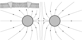
Figure 4: Two conical inclusions act as sources of a local membrane tilt (inset). The tilt-field-lines are illustrated qualitatively in this symmetric situation.

Following the same reasoning as for the geometrical forces discussed above, and remembering that the tilt vanishes on branch 3 so that its contribution vanishes, we find

$${\boldsymbol{F}}_{\operatorname{m}}=-\int_{1}{\operatorname{d}}s\;l_{a}T_{\operatorname{m}}^{ab}{\boldsymbol{e}}_{b}\ ,$$ (38)

with $T_{\operatorname{m}}^{ab}$ given by Eqn. (17). To simplify this expression, we need to have a close look at the symmetry. For this it is very helpful to again expand vectors and tensors in a local orthonormal frame $({\boldsymbol{l}},{\boldsymbol{t}})$, just as we have done in the geometrical case above. Mirror symmetry then informs us that $m^{\|}$ is an even function along the direction perpendicular to branch 1, while $m^{\perp}$ is an odd function and thus in particular zero everywhere on that branch. It thus follows that both $\nabla_{\perp}m^{\|}$ and $\nabla_{\|}m^{\perp}$ vanish everywhere on branch 1. Thus we have

$$M \stackrel{{\scriptstyle 1}}{{=}} (\nabla_{\perp}m^{\perp})+(\nabla_{\|}m^{\|})\ ,$$ (39a)

$$M_{ab}M^{ab} \stackrel{{\scriptstyle 1}}{{=}} (\nabla_{\perp}m^{\perp})^{2}+(\nabla_{\|}m^{\|})^{2}\ ,$$ (39b)

$$\varepsilon^{ab}\nabla_{a}m_{b} \stackrel{{\scriptstyle 1}}{{=}} \nabla_{\perp}m^{\|}-\nabla_{\|}m^{\perp}\;=\;0\ ,$$ (39c)

where the “$1$” above the equation signs reminds us that this only holds on branch 1. We next need to look at the contractions of the individual terms in the metric material stress with $l_{a}{\boldsymbol{e}}_{b}$. We find:

$$l_{a}(\nabla_{c}m^{a})(\nabla^{c}m^{b}){\boldsymbol{e}}_{b} \stackrel{{\scriptstyle 1}}{{=}} (\nabla_{\perp}m^{\perp})^{2}{\boldsymbol{l}}\ ,$$ (40a)

$$l_{a}(\nabla^{a}m_{c})(\nabla^{b}m^{c}){\boldsymbol{e}}_{b} \stackrel{{\scriptstyle 1}}{{=}} (\nabla_{\perp}m^{\perp})^{2}{\boldsymbol{l}}\ ,$$ (40b)

$$l_{a}MM^{ab}{\boldsymbol{e}}_{b} \stackrel{{\scriptstyle 1}}{{=}} M(\nabla_{\perp}m^{\perp})\,{\boldsymbol{l}}\ .$$ (40c)

The two terms involving the derivatives $m^{c}\nabla_{c}$ can be rewritten by extracting a total derivative:

$$l_{a}m^{c}(\nabla_{c}M)g^{ab}{\boldsymbol{e}}_{b} \stackrel{{\scriptstyle 1}}{{=}} {\boldsymbol{l}}\,m^{\|}\nabla_{\|}M$$ (41a)

$$\stackrel{{\scriptstyle 1}}{{=}} {\boldsymbol{l}}\big{[}\nabla_{\|}(m^{\|}M)-(\nabla_{\|}m^{\|})M\big{]}\ .\;\;\;\;\;\;$$

The total derivative will yield a boundary term once integrated along branch 1, and since we assume that we are not in a spontaneously tilted phase, $$|m^{a}|$$ will go to zero at infinity and thus the boundary term vanishes. With the same argument we find

$$l_{a}m^{c}(\nabla_{c}M^{ab}){\boldsymbol{e}}_{b} \stackrel{{\scriptstyle 1}}{{=}} {\boldsymbol{l}}\big{[}\nabla_{\|}(m^{\|}(\nabla_{\perp}m^{\perp}))$$ (41b)

$$-\,(\nabla_{\|}m^{\|})(\nabla_{\perp}m^{\perp})\big{]}\ .$$

Again, the total derivative integrates to zero. Finally, the potential terms simplify to

$$l_{a}V(m^{2})g^{ab}{\boldsymbol{e}}_{b} \stackrel{{\scriptstyle 1}}{{=}} V(m^{2})\,{\boldsymbol{l}}\ ,$$ (42a)

$$l_{a}V^{\prime}(m^{2})m^{a}m^{b}{\boldsymbol{e}}_{b} \stackrel{{\scriptstyle 1}}{{=}} 0\ .$$ (42b)

Collecting all results, we arrive at the remarkably simple exact force expression ${\boldsymbol{F}}_{\operatorname{m}}=F_{\operatorname{m}}{\boldsymbol{x}}$, with

$$F_{\operatorname{m}} = -\;\big{(}{\textstyle\frac{1}{2}}\lambda+\mu\big{)}\int_{1}{\operatorname{d}}s\;\Big{[}(\nabla_{\perp}m^{\perp})^{2}-(\nabla_{\|}m^{\|})^{2}\Big{]}$$ (43)

$$+\;\int_{1}{\operatorname{d}}s\;V(m^{2})\ .$$

There are two contributions to the force, one stemming from gradients of the tilt, the other from the tilt potential $V$. Remarkably, the tilt gradient contribution from each of the first two quadratic invariants has the same structural form, thus the Lamé coefficients $\lambda$ and $\mu$ occur only as a combination in front of the integral. The modulus $\nu$ has dropped out since the corresponding stress vanishes on the mid-curve (see Eqn. (39c)).

The structural similarity of Eqn. (43) to curvature mediated forces – Eqn. (33) – is very striking. Since $\frac{1}{2}\lambda+\mu>0$ Lame , the first integral states that perpendicular gradients of the perpendicular tilt lead to repulsion, while parallel gradients of the parallel tilt imply attractions – the same “$\perp^{2}-\|^{2}\,$” motif as found in Eqn. (33). Since in the untilted phase $V(m^{2})\geq 0$, the second line shows that the integrated excess potential drives attraction, just as the excess length (something like an integrated “surface tilt”) drives attraction in Eqn. (33). Unfortunately, the overall sign of the force is not obvious. Looking at the field lines in Fig. 4, the visual analogy with electrostatic interactions between like charged particles would suggest a repulsion, but the above analysis advises caution (in Sec. VI.3 we will see that this naive guess is at least borne out on the linearized level). Moreover, we should not forget that tilt does couple to geometry (namely, via the covariant derivative) and that the membrane by no means needs to be flat; hence, the contribution due to tension and bending given by Eqn. (33) must be added, the sign of which is equally unclear.

IV.4.3 Further geometric Hamiltonians

Within the framework of reparametrization invariant Hamiltonians providing a scalar energy density, a systematic power series in terms of all available scalars and their covariant derivatives (each multiplying some phenomenological “modulus”) is a formal (and in fact standard) way of obtaining an energy expression of a physical system. In this respect the Hamiltonian (24) is no exception, being simply the quadratic expansion for an up-down symmetric surface (notice that a term proportional to $K$ would break this symmetry, giving rise to a spontaneous curvature). We hasten to add that a second quadratic term, proportional to the Gaussian (or Ricci) curvature, exists as well, but this usually plays no role since it only results in a topological invariant (see also the Appendix).

The fact that curvature (a “generalized strain”) enters quadratically in the Hamiltonian (24) classifies this form of the bending energy as “linear curvature elasticity” (even though the resulting shape equations are highly nonlinear). However, for sufficiently strong bending higher than quadratic terms will generally contribute to the energy density, giving rise to genuinely nonlinear curvature elasticity GoeHel96 . Nevertheless, such effects pose no serious problem for the approach we have outlined so far. In fact, they are incorporated very naturally. We would like to illustrate this with two examples.

a. Quartic curvature. Sticking with up-down symmetric surfaces, the next curvature order would be quartic, and this gives rise to three more scalars: $K^{4}$, $K^{2}R$ and $R^{2}$. Let us for simplicity only study the case of a quartic contribution of the form

$$\mathcal{H}_{4}=\frac{1}{4}\kappa_{4}K^{4}\ .$$ (44)

Using the general expression of the stress tensor for the scalar $K^{n}$ as calculated in the Appendix (see Eqn. (86)) and going through the calculation from Sec. IV.4 we find for instance

$$F_{\text{sym,cyl}}/L=-\frac{3}{4}\kappa_{4}K_{\perp}^{4}\ ,$$ (45)

if two parallel cylinders adhere to the same side of the interface. This term increases the repulsion between cylinders found on the linear elastic level (see Eqn. (34)), provided $\kappa_{4}>0$, i. e., provided the quartic term further stiffens the membrane.

Assuming that $\mathcal{H}_{4}$ perturbs the usual bending Hamiltonian $\frac{1}{2}\kappa K^{2}$, we can use the two moduli to define a characteristic length scale $\ell_{4}:=\sqrt{|\kappa_{4}|/\kappa}$. The overall force up to quartic order can then be written as

$$F_{\text{sym,cyl}}/L=-\frac{1}{2}\kappa K_{\perp}^{2}\,\Big{[}1\pm\frac{3}{2}(\ell_{4}K_{\perp})^{2}\Big{]}\ ,$$ (46)

where the $+$-sign corresponds to stiffening. Notice that the correction term becomes only noticeable once the curvature radius of the membrane is no longer large compared to the length scale $\ell_{4}$. It appears natural that $\ell_{4}$ is related to the membrane thickness, which for phospholipid bilayers is about $5\,\text{nm}$. Assuming a (quadratic order) bending stiffness of $\kappa\simeq 20\,k_{\text{B}}T$, we thus expect values for the modulus $\kappa_{4}$ on the order of $10^{3}\,k_{\text{B}}T\,\text{nm}^{2}$.

b. Curvature gradients. In order length^-4 it is possible to also generate scalars which depend on derivatives of the surface curvature. One such term is

$$H_{\nabla}=\frac{1}{2}\kappa_{\nabla}(\nabla_{a}K)(\nabla^{a}K)\ .$$ (47)

Using the expression for the stress tensor derived in the Appendix (see Eqn. (96)) and again going through the calculation in Sec. IV.4, we find

$$F_{\text{sym,cyl}}/L=\frac{1}{4}\kappa_{\nabla}\nabla_{\perp}^{2}K_{\perp}^{2}=\frac{1}{4}\kappa_{\nabla}\frac{{\operatorname{d}}^{2}}{{\operatorname{d}}l^{2}}K_{\perp}^{2}$$ (48)

for the force between two symmetrically adhering cylinders. It depends on very subtle details of the membrane shape: the curvature is (roughly) a second derivative of the membrane position, and this we need to square and differentiate two more times. Unfortunately, the sign of the interaction is not obvious here, as the second derivative of $K_{\perp}^{2}$ with respect to $l$ may be either positive or negative. Finally, we can also define a characteristic length scale here, $\ell_{\nabla}:=\sqrt{|\kappa_{\nabla}|/\kappa}$. The importance of a perturbation $\mathcal{H}_{\nabla}$ of the usual bending Hamiltonian depends on whether or not the curvature changes significantly on length scales comparable to $\ell_{\nabla}$.

V Description of the surface in Monge parametrization

In the previous section analytical expressions for the force between two attached particles have been derived which link the force to the geometry of the surface at the midplane between them. It is worthwhile reemphasizing that they are exact, even in the nonlinear regime. In special cases, the sign of the interaction is also revealed.

If one is interested in quantitative results, however, shape equations need to be solved – numerically or analytically. Either way, one needs to pick a surface parametrization. The choice followed in essentially all existing calculations in the literature is “Monge gauge”, and for analytical tractability its linearized version. The purpose of this and the following section is to translate the general covariant formalism developed so far into this more familiar language. To this end we first remind the reader what the basic geometric objects look like in this gauge. We are then in a position to quantitatively study three different examples of interface mediated interactions in Sec. VI.

V.1 Definition and properties

Any surface free of “overhangs” can be described in terms of its height $h(x,y)$ above some reference plane, which we take to be the $(x,y)$ plane. Notice that $x$ and $y$ thus become the surface coordinates. The direction of the basis vectors $\{{\boldsymbol{x}},{\boldsymbol{y}},{\boldsymbol{z}}\}\in\mathbb{R}^{3}$ is as described in Sec. IV.3.

The tangent vectors on the surface are then given by ${\boldsymbol{e}}_{x}=(1,0,h_{x})^{\top}$ and ${\boldsymbol{e}}_{y}=(0,1,h_{y})^{\top}$, where $h_{i}=\partial_{i}h$ ($i,j\in\{x,y\}$). The metric is given by

$$g_{ij}=\delta_{ij}+h_{i}h_{j}\ ,$$ (49)

where $\delta_{ij}$ is the Kronecker symbol. Observe that $g_{ij}$ is not diagonal; even though the coordinates $\{x,y\}$ refer to an orthonormal coordinate system on the base plane, this property does not transfer to the surface they parameterize. We also define the gradient operator in the base plane, ${\boldsymbol{\nabla}}:=(\partial_{x},\partial_{y})^{\top}$. The metric determinant can then be written as $g=|g_{ij}|=1+({\boldsymbol{\nabla}}h)^{2}$, and the inverse metric is given by $g^{ij}=\delta_{ij}-h_{i}h_{j}/g$. It is, perhaps, worth emphasizing that the latter, just as Eqn. (49), are not tensor identities. The right-hand side gives the numerical values of the components of the covariant tensors $g_{ij}$ and $g^{ij}$ with respect to the coordinates $x$ and $y$.

The unit normal vector is equal to

$${\boldsymbol{n}}=\frac{1}{\sqrt{g}}\left(\begin{array}[]{c}-{\boldsymbol{\nabla}}h\\ 1\end{array}\right)\ .$$ (50)

With the help of Eqn. (1) the extrinsic curvature tensor is determined to be:

$$K_{ij}=-\frac{h_{ij}}{\sqrt{g}}\ ,$$ (51)

where $h_{ij}=\partial_{i}\partial_{j}h$. Note that Eqn. (51) again is not a tensor equation; it provides the numerical values of the components of $K_{ij}$ in Monge gauge.

Finally, it is also possible to write the trace $K$ of the extrinsic curvature tensor in Monge parametrization:

$$K=-{\boldsymbol{\nabla}}\cdot{\Big{(}\frac{{\boldsymbol{\nabla}}h}{\sqrt{g}}}\Big{)}\ .$$ (52)

V.2 Small gradient expansion

In Sec. VI we will be interested in surfaces that deviate only weakly from a flat plane. In this situation the gradient ${\boldsymbol{\nabla}}h$ is small, and it is sufficient to consider only the lowest nontrivial order of a small gradient expansion. $K$ and ${\operatorname{d}}A$ can then be written as

$$K = -{\boldsymbol{\nabla}}^{2}h+\mathcal{O}[({\boldsymbol{\nabla}}h)^{2}]\ ,$$ (53)

$${\operatorname{d}}A = {\Big{\{}1+\frac{1}{2}({\boldsymbol{\nabla}}h)^{2}+\mathcal{O}[({\boldsymbol{\nabla}}h)^{4}]}\Big{\}}\;{\operatorname{d}}x\;{\operatorname{d}}y\ .$$ (54)

To evaluate the line integrals described in Sec. IV.4 we need expressions for $K_{\perp}$ and $K_{\|}$ as well as the derivatives $\nabla_{\perp}K_{\perp}$ and $\nabla_{\perp}K_{\|}$ at branch 1 in Monge parametrization. In the small gradient expansion, the result is simply

$$K_{\perp} = -h_{xx}(0,y)\ ,$$ (55a)

$$K_{\|} = -h_{yy}(0,y)\ ,$$ (55b)

as well as

$$\nabla_{\perp}K_{\perp} = -h_{xxx}(0,y)\ ,$$ (56a)

$$\nabla_{\perp}K_{\|} = -h_{yyx}(0,y)\ .$$ (56b)

We are now in a position to determine the forces between two particles in different situations.

VI Examples

In this section we will illustrate the general framework of geometry-encoded forces by treating three important examples in Monge gauge: capillary, curvature mediated, and tilt-induced interactions. For the first two, force-distance curves have previously been derived on the linearized level pinningexp ; pinningtheo ; Weiklcyl . The route via the stress tensor reproduces these results with remarkable ease, thereby underscoring its efficiency and also confirming its validity (at least on the linear level). To illustrate tilt-mediated interactions we restrict to a simplified situation in which we neglect the coupling of membrane shape and tilt-order. Even if the geometry is “trivial” (a flat membrane), the material stress tensor is not, and forces remain.

Both geometric examples are special cases of the Hamiltonian density (24). When the gradients are small, the surface energy is given by the quadratic expression:

$$H=\frac{1}{2}\int{\operatorname{d}}x\;{\operatorname{d}}y\;{\Big{[}\kappa({\boldsymbol{\nabla}}^{2}h)^{2}+\sigma({\boldsymbol{\nabla}}h)^{2}}\Big{]}\ .$$ (57)

If $\kappa=0$ this describes a soap film; if $\kappa\neq 0$ it will describe a fluid membrane.

The approach, traditionally followed in the literature, is to first determine the surface profile $h(x,y)$ which minimizes the energy Eqn. (57). For this one must solve the linear Euler-Lagrange equation

$${\boldsymbol{\nabla}}^{2}\big{(}{\boldsymbol{\nabla}}^{2}-\ell^{-2}\big{)}\,h(x,y)=0\ ,$$ (58)

where $\ell$ is the length from Eqn. (25). In a next step, the energy corresponding to this shape is evaluated by reinserting the solution of Eqn. (58) into the functional (57). This energy will depend on the relative positions of the bound objects. Appropriate derivatives of the energy with respect to these positions will yield the forces between the particles. By contrast our approach — sidestepping the need to evaluate the energy — will be to determine the force directly from the surface profile using the line integral expressions for the force, Eqns. (33) and (35).

VI.1 Soap films

For a soap film, $\kappa=0$ and thus $\ell=0$. The relevant Euler-Lagrange equation is therefore the Laplace equation, ${\boldsymbol{\nabla}}^{2}h=0$.

Consider first the symmetrical configuration consisting of two parallel cylindrical particles which adhere to one side of the soap film. Eqn. (33) indicates that, if we neglect end effects, the force between the cylinders is proportional to the excess length on branch 1. The excess length, however, is zero because the contact lines are straight. Therefore, the force is also zero. Likewise, in the antisymmetric configuration with adhesion on opposite sides, the soap film between the cylinders will be flat if the vertical particle displacements are allowed to equilibrate. Therefore, $\varphi(s)=0$ (see Fig. 3) and Eqn. (35) will yield a zero force exactly as in the symmetric case. In an analogous way one obtains the same result for the case of two spheres.

The situation is less simple if the film is pinned to the particle surface. Let us consider two spherical particles of radius $a$ with a contact line that departs only weakly from a circle.

Stamou et al. pinningexp have studied this case by using a superposition ansatz in the spirit of Nicolson nicolson : first, the height function of one isolated particle is determined with the correct boundary conditions. Then, the complete height function is assumed to be the sum of the two single-particle fields of each of the two colloids. Strictly speaking, this approach destroys the boundary conditions at the particles’ contact lines; it does, however, give the correct leading order result for large separation exactsolution .

Using polar coordinates $\rho$ and $\phi$, the solution of the shape equation outside a single spherical particle can be written as pinningexp

$$h_{\text{sphere}}(\rho,\phi) = A_{0}\ln{{\Big{(}\frac{a}{\rho}}\Big{)}}$$ (59)

$$+\sum_{m=1}^{\infty}A_{m}\cos{[m(\phi-\phi_{m,0})]}{\Big{(}\frac{a}{\rho}}\Big{)}^{m}\ ,\;\;\;\;\;\;\;$$

with multipole coefficients $A_{m}$ and phase angles $\phi_{m,0}$. The former can be determined as follows: The monopole $A_{0}$ vanishes because there is no external force such as gravity pulling on the particle. The dipole coefficient $A_{1}$ characterizes the tilt of the contact line relative to the ${\boldsymbol{z}}$ axis; it also vanishes if there is no external torque acting on the sphere. All higher multipole coefficients can be read off from the Fourier expansion of the contact line at $\rho=a$. It is intuitively obvious and indeed confirmed by a more careful calculation pinningexp ; pinningtheo that the quadrupole dominates the energy at lowest order.

One can therefore restrict the calculation to the single-particle height function pinningexp

$$h_{\text{sphere}}(\rho,\phi)=Q\cos[2(\phi-\phi_{0})]{\Big{(}\frac{a}{\rho}}\Big{)}^{2}\ ,$$ (60)

where $\phi_{0}:=\phi_{2,0}$ is the angle that represents the rotation of the particle about ${\boldsymbol{z}}$ (see Fig. 5).

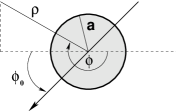
Figure 5: Definition of the coordinates for a single quadrupole (viewed from above).

If the complete height function is a superposition, as described above, the force on the left particle in lowest order has been found to be pinningexp ; pinningtheo

$${\boldsymbol{F}}_{\text{sym,soap}}=-{\boldsymbol{F}}_{\text{antisym,soap}}=48\pi\sigma Q^{2}\frac{a^{4}}{d^{5}}{\boldsymbol{x}}\ ,$$ (61)

for the symmetric ($\phi_{0,{\text{A}}}=-\phi_{0,{\text{B}}}$) and the antisymmetric ($\phi_{0,{\text{A}}}=0,\;\phi_{0,{\text{B}}}=\pi/2$) configurations (see Fig. 6).

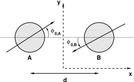
Figure 6: Two quadrupoles on a soap film (viewed from above).

Let us now examine the same two configurations using the line integral representation for the force.

a. Symmetric case. The force Eqn. (33) is proportional to the excess length of branch 1 with respect to branch 3. To quadratic order in gradients, this difference can be written as

$$\Delta L = \lim_{L\rightarrow\infty}{\Big{\{}\int_{-L/2}^{L/2}{\operatorname{d}}y\;{\Big{[}\sqrt{1+h_{y}^{2}(0,y)}-1}}\Big{]}\Big{\}}$$ (62)

$$= \lim_{L\rightarrow\infty}{\Big{\{}\int_{-L/2}^{L/2}{\operatorname{d}}y\;\Big{[}\frac{1}{2}h_{y}^{2}(0,y)+\mathcal{O}[({\boldsymbol{\nabla}}h)^{4}]\Big{]}}\Big{\}}\ .\;\;\;\;\;\;\;$$

The height function along the symmetry line between the particles can be expressed in Cartesian coordinates as:

$$h(0,y)=2Q\cos\Big{[}2\Big{(}\arctan{\frac{2y}{d}}+\phi_{0,{\text{A}}}\Big{)}\Big{]}\frac{a^{2}}{y^{2}+\frac{d^{2}}{4}}\ .$$ (63)

Substituting into the second line of Eqn. (62) gives

$$\Delta L = \lim_{L\rightarrow\infty}\Big{[}96Q^{2}\frac{a^{4}}{d^{5}}\arctan{\frac{L}{d}}+\mathcal{O}(L^{-1})\Big{]}$$ (64)

$$= 48\pi Q^{2}\frac{a^{4}}{d^{5}}\ ,$$

implying via $F_{\text{sym,soap}}=\sigma\Delta L$ the same force as obtained from energy minimization, Eqn. (61). However, it would be fair to say that we have gained additional information concerning the nature of this force, missing before. The force is directly proportional to the length added to the mid-curve as it is stretched. A geometrical interpretation has been provided for the force. Recall also that this is a non-perturbative result: it does not depend on the small gradient approximation.

b. Antisymmetric case. In this case the horizontal force is given by Eqn. (35) with $\kappa=0$:

$$F_{\text{antisym,soap}}=\sigma\lim_{L\rightarrow\infty}{\Big{\{}\int_{-L/2}^{L/2}{\operatorname{d}}y\;{\Big{[}{\boldsymbol{n}}\cdot{\boldsymbol{z}}-1}\Big{]}}\Big{\}}$$

$$=\sigma\lim_{L\rightarrow\infty}{\Big{\{}\int_{-L/2}^{L/2}{\operatorname{d}}y{\Big{[}\frac{1}{\sqrt{1+h_{x}^{2}(0,y)}}-1}\Big{]}}\Big{\}}$$

$$=\sigma\lim_{L\rightarrow\infty}{\Big{\{}\int_{-L/2}^{L/2}{\operatorname{d}}y{\Big{[}-\frac{1}{2}h_{x}^{2}(0,y)+\mathcal{O}[({\boldsymbol{\nabla}}h)^{4}]}\Big{]}}\Big{\}}\ .\;\;\;\;\;\;\,$$ (65)

The height function between the particles is given by

$$h(x,y) = Qa^{2}\times$$ (66)

$$\bigg{\{}\frac{\cos{[2(\arctan{\frac{y}{\frac{d}{2}+x}})]}}{y^{2}+(\frac{d}{2}+x)^{2}}-\frac{\cos{[2(\arctan{\frac{y}{\frac{d}{2}-x}})]}}{y^{2}+(\frac{d}{2}-x)^{2}}\bigg{\}}\ ,$$

so that

$$h_{x}(0,y)=-\frac{32Qa^{2}d(d^{2}-12y^{2})}{(d^{2}+4y^{2})^{3}}\ .$$ (67)

Inserting this into Eqn. (65) yields a force which again agrees with the one obtained in Eqn. (61).

As an example, let us look at colloids with a radius of $1\,\mu\text{m}$ trapped at the air-water interface ($\sigma\simeq 70\,\text{mN}/\text{m}$), which have a pinning quadrupole of 1% of their radius ($Q\simeq 10\,\text{nm}$). At a separation of $3\,\mu\text{m}$ they feel an (attractive or repulsive) force of $1\,\text{pN}$, and at a separation of about $16\,\mu\text{m}$ their interaction energy is comparable to the thermal energy. These forces are not particularly strong, but they act over an exceptionally long range.

VI.2 Fluid Membranes

To describe a fluid membrane, it is necessary to include the bending energy in Eqn. (57). Let us focus on the problem of two parallel adhering cylinders which are sufficiently long so that end effects can be neglected (the fluid membrane analogue of the problem examined for soap films). In this case the height function of the surface depends only on one variable, $x$. Recall that for the corresponding soap film case no interaction occurred (in the absence of pinning), see Sec. VI.1.

a. Symmetric case. Using the energy route, Weikl Weiklcyl shows that, at lowest order in the small gradient expansion, the energy per unit length of the cylinder is go_to_zero

$$E_{\text{sym,cyl}}(d)=-\frac{(\kappa+2R^{2}U)^{2}(\tanh\frac{d}{2\ell}-1)}{4\sqrt{\sigma\kappa}R^{2}}\ .$$ (68)

Here $R$ is the cylinder radius, $U$ is the adhesion energy per unit area, $\ell$ is the characteristic length defined in Eqn. (25), and $d$ is the distance between the two centers of the cylinders. To obtain the force per unit length $L$ of the left cylinder, we differentiate Eqn. (68) with respect to $d$ sign_of_force :

$$F_{\text{sym,cyl}}/L=-\frac{1}{2}\kappa\bigg{(}\frac{\kappa+2R^{2}U}{2\kappa R\cosh\frac{d}{2\ell}}\bigg{)}^{2}\ .$$ (69)

The cylinders always repel.

We would now like to determine the force using the line integral of the corresponding stress tensor. Rewriting the relevant Eqn. (34) in small gradient expansion yields (see Eqn. (55a)):

$$F_{\text{sym,cyl}}/L\;=\;-\frac{1}{2}\kappa h_{xx}^{2}(0)\ .$$ (70)

We use the expression for $h$ given in Ref. Weiklcyl :

$$h(x)=\frac{(\kappa+2R^{2}U)\cosh{\frac{x}{\ell}}}{2\sigma R\cosh{\frac{d}{2\ell}}}+\text{const}\ .$$ (71)

Its second derivative with respect to $x$ at $x=0$ is

$$h_{xx}(0)=\frac{\kappa+2R^{2}U}{2\kappa R\cosh{\frac{d}{2\ell}}}\ .$$ (72)

Inserting this result into Eqn. (70) reproduces the force given by Eqn. (69).

b. Antisymmetric case. For two cylinders on opposite sides of the membrane the energy is given by Weiklcyl ; go_to_zero

$$E_{\text{antisym,cyl}}(d)=-\frac{(\kappa+2R^{2}U)^{2}(\coth\frac{d}{2\ell}-1)}{4\sqrt{\sigma\kappa}R^{2}}\ ,$$ (73)

which gives a force on the left cylinder sign_of_force

$$F_{\text{antisym,cyl}}/L=\frac{1}{2}\kappa\bigg{(}\frac{\kappa+2R^{2}U}{2\kappa R\sinh\frac{d}{2\ell}}\bigg{)}^{2}\ .$$ (74)

The small gradient expansion of Eqn. (37) is

$$F_{\text{antisym,cyl}}/L=\frac{1}{2}\kappa\,(\ell\nabla_{\perp}K_{\perp})^{2}\stackrel{{\scriptstyle(\ref{eq:KperpderperpMongesmallgradient})}}{{=}}\frac{1}{2}\kappa\,[\ell h_{xxx}(0)]^{2}\ .$$ (75)

If we now again take the height function from Ref. Weiklcyl we arrive at

$$h(x)=\frac{(\kappa+2R^{2}U)\sinh{\frac{x}{\ell}}}{2\sigma R\sinh{\frac{d}{2\ell}}}\ ,$$ (76)

which yields

$$\ell h_{xxx}(0)=\frac{\kappa+2R^{2}U}{2\kappa R\sinh{\frac{d}{2\ell}}}\ .$$ (77)

Inserting this into Eqn. (75) reproduces the result (74).

How big are these forces? As an example, let us look at an actin filament ($R\simeq 4\,\text{nm}$) adsorbed onto a membrane with a typical bending stiffness $\kappa\simeq 20\,k_{\text{B}}T$, where $k_{\text{B}}T$ is the thermal energy. Noting that $\sqrt{2U/\kappa}$ will be the contact curvature at the point where the membrane detaches from the adsorbing filament SeLi90 and that this should not be too much smaller than the bilayer thickness in order for a Helfrich treatment to be permissible, we take $2UR^{2}/\kappa\simeq 1$ as an upper limit. We then find that two adsorbed actin filaments at a distance $d\simeq\ell$ (where approximately $\sinh\approx\cosh\approx 1$) feel a force of about $2-3\,\text{pN}/\text{nm}$. Alternatively, we can calculate at what distance the interaction energy per persistence length of the filament ($\ell_{\operatorname{p}}\approx 15\,\mu\text{m}$) is of order $k_{\text{B}}T$. Using a typical value for cell membranes of $\ell\approx 50\,\text{nm}$, we obtain a separation of about $0.7\,\mu\text{m}$. This is huge, and should remind us of the fact that on this scale a lot of membrane fluctuations will occur which we have neglected. Still, it shows rather vividly that membrane mediated forces can be very significant.

VI.3 Lipid tilt

The discussion in Sec. III shows that lipid tilt order, described by the surface vector field $m^{a}$, influences the shape of the membrane, even if the Hamiltonian density does not contain an explicit coupling of $m^{a}$ to the extrinsic curvature. The coupled system of differential equations (18) poses a formidable task, clearly exceeding the already substantial one for the undecorated shape equation alone.

Our priority is to illustrate the workings of the general formalism, therefore we will limit the discussion to a simple case where the analytical treatment is rather transparent: we will assume that the membrane itself remains flat, such that the energy density stems exclusively from lipid tilt (as described by $\mathcal{H}_{\operatorname{m}}$ from Eqn. (16)). This is not a self-consistent approximation, but should give a good description in the limit in which the tilt moduli $\lambda$ and $\mu$ are significantly “softer” than the bending modulus. In this case the inclusions we have talked about in Sec. IV.4.2 will predominantly excite tilt and not bend. More sophisticated (analytical and numerical) studies of lipid tilt and mediated interactions exist, which provide better quantitative answers tilt_force .

For flat membranes, the Euler-Lagrange equation (19) reduces to

$$(\lambda+\mu){\boldsymbol{\nabla}}{\boldsymbol{\nabla}}\cdot{\boldsymbol{m}}+\mu{\boldsymbol{\nabla}}^{2}{\boldsymbol{m}}-2V^{\prime}{\boldsymbol{m}}=0\ ,$$ (78)

where ${\boldsymbol{m}}$ is the 2d tilt vector in the membrane plane. Focusing first on one inclusion, the situation acquires cylindrical symmetry. Writing ${\boldsymbol{m}}({\boldsymbol{r}})=m(r){\boldsymbol{e}}_{r}$ and restricting to the untilted membrane phase, for which the tilt potential is sufficiently well represented by $V(m^{2})=\frac{1}{2}tm^{2}$ with $t>0$, Eqn. (78) reduces to a simple Bessel equation

$$x^{2}m^{\prime\prime}+xm^{\prime}-(x^{2}+1)m=0\ ,$$ (79)

where $x=r/\ell_{\operatorname{m}}$, $\ell_{\operatorname{m}}$ is the length defined in Eqn. (23), and the prime denotes a derivative with respect to $x$. The solution is

$$m(r)=m_{0}\frac{K_{1}(r/\ell_{\operatorname{m}})}{K_{1}(r_{0}/\ell_{\operatorname{m}})}\ ,$$ (80)

where $r_{0}$ is the radius of the inclusion, $m_{0}$ the value of the tilt at this point, and $K_{\nu}$ a modified Bessel function of the second kind abramowitz . As anticipated, the tilt decays essentially exponentially with a decay length of $\ell_{\operatorname{m}}$.

Obtaining the exact tilt field for two inclusions is very difficult, since satisfying the boundary conditions is troublesome. However, if we again use the Nicolson approximation nicolson and assume that the total tilt distribution is given by the superposition of two solutions of the kind (80), things become manageable. The tilt-mediated force between two symmetric inclusions is then obtained by inserting the appropriate values and derivatives of the tilt field ${\boldsymbol{m}}(x,y)$ on the mid-line into Eqn. (43). After some straightforward calculations we get the force integral

$$F_{\operatorname{m}} = 4t\ell_{\operatorname{m}}m_{0}^{\ast 2}\int_{d^{\ast}}^{\infty}{\operatorname{d}}\xi\;\frac{1}{\xi\sqrt{\xi^{2}-d^{\ast 2}}}\times$$ (81)

$$\Big{[}(\xi^{2}-2d^{\ast 2})K_{0}(\xi)K_{2}(\xi)+(\xi^{2}-d^{\ast 2})K_{1}^{2}(\xi)\Big{]}$$

$$= -2\pi t\ell_{\operatorname{m}}m_{0}^{\ast 2}\,K_{1}(d/\ell_{\operatorname{m}})\ .$$

where $m_{0}^{\ast}=m_{0}/K_{1}(r_{0}/\ell_{\operatorname{m}})$, $d^{\ast}=d/2\ell_{\operatorname{m}}$, and $d$ is the separation between the inclusions. As we see, the force is repulsive and decays essentially exponentially with distance over a decay length of $\ell_{\operatorname{m}}$. Integrating it, we get the repulsive interaction potential

$$U_{\operatorname{m}}(d)=2\pi t\ell_{\operatorname{m}}^{2}m_{0}^{\ast 2}\,K_{0}(d/\ell_{\operatorname{m}})\ .$$ (82)

Let us try to make a very rough estimate of how big such a force might be. For this we need to obtain some plausible values for the numbers entering into Eqn. (81). For $t$ we may use the equipartition theorem and argue that $\frac{1}{2}t\langle m^{2}\rangle a=\frac{1}{2}k_{\text{B}}T$, where $a$ is the area per lipid and $k_{\text{B}}T$ the thermal energy. Assuming that the root-mean-square fluctuations of $m$ are $10^{\circ}$ and using the typical value $a\simeq 0.75\,\text{nm}^{2}$, we get $t\simeq 40\,k_{\text{B}}T/\text{nm}^{2}$. Assuming further a rather conservative tilt decay length of the order of the bilayer thickness, i. e. $\ell_{\operatorname{m}}\simeq 5\,\text{nm}$, that the inclusion has a radius of $r_{0}\simeq 3\,\text{nm}$ and imposes there a local tilt of $m\simeq 0.2$, we find that two inclusions at a distance of $10\,\text{nm}$ feel a significant force of about $17\,\text{pN}$. And at a distance of $d\approx 22\,\text{nm}$ their mutual potential energy is $1\,k_{\text{B}}T$ compared to the separated state. Notice that this is much larger than the Debye length in physiological solution, which is typically only $1\,\text{nm}$. Hence, tilt-mediated forces can compete with more conventional forces, such as (screened) electrostatic interactions. It should be kept in mind, however, that if we permit the membrane to bend, some of the tilt strain can be relaxed, thereby lowering the energy.

VII Conclusions

We have shown how the stress tensor can be used to relate the forces between particles bound to an interface directly to the interface geometry. In this approach, the force on a particle is given by a line integral of the stress along any closed contour surrounding the particle. The stress depends only on the local geometry; thus the force is completely encoded in the surface geometry in the neighborhood of the curve.

The relationship between the force and the geometry provided by the line integral is exact. In the linear regime, as we have shown for selected examples in the previous section, the force determined by evaluating this line integral reproduces the result obtained by the more familiar energy based approach. Unlike the latter, however, our approach permits us to consider large deformations. The expression for the line-integral is fully covariant, involving geometrical tensors; one is not limited to any one particular parametrization of the surface such as the Monge gauge. Indeed, as we have seen the geometrical origins of the force can get lost in this gauge.

As we have emphasized previously, this approach is not a substitute for solving the nonlinear field equations. To extract numbers, we do need to solve these equations. But even before this is done, the line integral expression can provide valuable qualitative information concerning the nature of the interactions between particles. This is because the geometry along the contour is often insensitive to the precise conditions binding the particle to the interface. This contrasts sharply with the energy based approach; there, one needs to know the entire distribution of energy on the interface before one can say anything about the nature of the interaction. As we have seen in the context of a symmetrical two-particle configuration, it is sometimes relatively easy to identify qualitative properties of the geometry; it is virtually impossible to make corresponding statements about the energy outside the linear regime.

The stress tensor approach also has the virtue of combining seamlessly with any approach we choose, be it analytical or numerical, to determine the surface shape. Thus, for instance, one can find surfaces that minimize a prescribed surface energy functional using the program “Surface Evolver” Brakke . The evaluation of the force via a line integral involving the geometry along the contour is straightforward; in contrast, the evaluation of the energy involves a surface integral, and the forces then follow by a subsequent numerical differentiation. In other words, the route via the energy requires one more integration but also one more differentiation. This appears neither economical nor numerically robust.

We have illustrated how internal degrees of freedom on the membrane can be incorporated within this approach using a vector order parameter describing lipid tilt as an example. It is indeed remarkable just how readily non-geometrical degrees of freedom can be accommodated within this geometrical framework. Here again, new exact non-linear expressions for the force between particles mediated by the tilt are obtained which are beyond the scope of the traditional approach to the problem. Various patterns emerge which could not have been guessed from inspection of the Hamiltonian, in particular the existence of a “$\perp^{2}-\|^{2}\,$” motif common to the geometrical and tilt mediated forces between symmetrical particles.

We have considered the force between a pair of particles. However, the interaction between more than two particles is generally not expressible as a sum over pairwise interactions; superposition does not hold if the theory is nonlinear (see Ref. Kim for a striking illustration). This, however, poses no difficulty for the stress tensor approach, because the underlying relation between surface geometry and force is independent of whether or not a pair-decomposition is possible (see Fig. 7). For certain symmetric situations a clever choice of the contour of integration may again yield expressions for the force analogous to those obtained in Sec. IV.4.

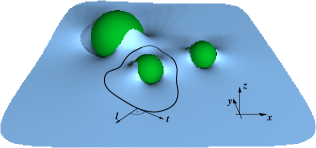
Figure 7: Three-body interactions. The force on one particle can be obtained by integrating the surface stress tensor along a line of integration enclosing that particle. (cf. Eqn. (12)).

Multi-body effects become particularly relevant when one considers 2D bulk phases as, for instance, in a system consisting of a large number of mutually repulsive particles adhering to one side of an interface. In this case it is possible to identify expressions for state variables such as the lateral pressure by exploiting the approach which has been introduced here.

The interfaces we have considered are asymptotically flat and thus support no pressure difference. At first glance it may appear that our approach fails if there is pressure because the stress tensor is no longer divergence free on the free surface (one has $\nabla_{a}{\boldsymbol{f}}^{a}=P{\boldsymbol{n}}$) which would obstruct the deformation of the contour described in Sec. IV.3. As we will show in a forthcoming publication, however, it is possible to adapt our approach to accommodate such a situation.

The interactions we have examined correspond to particles whose orientations are in equilibrium. The additional application of an external torque (e. g. on two dipoles via a magnetic field) will introduce a bending moment. It is, however, possible to treat such a situation with the tools provided in Ref. surfacestresstensor : Just as translational invariance gives us the stress tensor, rotational invariance gives us a torque tensor. Its contour integrals provide us with the torque acting on the patch one encircles.

Finally, genuine capillary forces involve gravity. The associated energy, however, depends not only on the geometry of the surface but also on that of the bulk (it is a volume force). The results thus differ qualitatively from those presented here. This will be the subject of future work.

Appendix A

In Sec. II.4 we derived the general expression

$${\boldsymbol{f}}^{a}=(T^{ab}-\mathcal{H}^{ac}K_{c}^{\;b}){\boldsymbol{e}}_{b}-\nabla_{b}\mathcal{H}^{ab}{\boldsymbol{n}}$$ (83)

for the surface stress tensor. In this appendix we will specialize (83) to a few important standard cases.

a. Area. The simplest case is the area, $\mathcal{H}=1$, which is (up to a constant prefactor) the Hamiltonian density of a soap film. We evaluate $\mathcal{H}^{ab}$ and $T^{ab}$ appearing in Eqn. (83) using Eqn. (7): $\mathcal{H}^{ab}=\delta\mathcal{H}/\delta K_{ab}=0$ and $T^{ab}=-g^{ab}$; for $T^{ab}$ we use the identity

$$\frac{\partial\sqrt{g}}{\partial g_{ab}}=\frac{1}{2}\sqrt{g}\,g^{ab}\ .$$ (84)

Thus we get

$${\boldsymbol{f}}^{a}=-g^{ab}{\boldsymbol{e}}_{b}\ .$$ (85)

Note that the functional derivatives $\delta$ in this case are equal to partial derivatives $\partial$ because $\mathcal{H}$ does not depend on higher derivatives of $g_{ab}$ or $K_{ab}$.

b. Powers of $K$. For the Hamiltonian density $\mathcal{H}=K^{n}=(g^{ab}K_{ab})^{n}$ one derives diffapp1 : $\mathcal{H}^{ab}=nK^{n-1}g^{ab}$ and $T^{ab}=2nK^{n-1}K^{ab}-K^{n}g^{ab}$ which gives

$${\boldsymbol{f}}^{a}=(nK^{n-1}K^{ab}-K^{n}g^{ab}){\boldsymbol{e}}_{b}-n(\nabla^{a}K^{n-1}){\boldsymbol{n}}\ .$$ (86)

The case $n=2$ is needed in Eqn. (24).

c. Einstein-Hilbert action. Canham Canham originally used the quadratic Hamiltonian $\mathcal{H}=K_{ab}K^{ab}$. For this one we easily see that $\mathcal{H}^{ab}=2K^{ab}$ and $T^{ab}=-\mathcal{H}g^{ab}+4K^{a}_{c}K^{bc}$ diffapp1 . Using the contractions of both Gauss-Codazzi-Mainardi equations (3) as well as the fact that the Euler-Lagrange derivative $\mathcal{E}(\mathcal{H})$ is linear in the Hamiltonian, we get with the help of Eqn. (9) the Euler-Lagrange derivative of the Einstein-Hilbert action, $\mathcal{H}=R$:

$$\mathcal{E}(R)=\mathcal{E}(K^{2})-\mathcal{E}(K_{ab}K^{ab})=-2K^{ab}G_{ab}\ .$$ (87)

Here, $G_{ab}=R_{ab}-\frac{1}{2}Rg_{ab}$ is the Einstein tensor, which vanishes identically in two dimensions. Thus, surface variations of $K^{2}$ and $K_{ab}K^{ab}$ differ only by boundary terms (in accord with the Gauss-Bonnet theorem DifferentialGeometry ). In higher dimensions, however, $\mathcal{E}(R)\propto G_{ab}$ is a nontrivial result, and the above seemingly inelegant (since extrinsic) derivation is after all remarkably economical.

d. Curvature gradient. The next example we consider is the Hamiltonian density $\mathcal{H}=\frac{1}{2}(\nabla_{c}K)(\nabla^{c}K)\equiv\frac{1}{2}(\nabla K)^{2}$. Now we need to keep in mind that $\mathcal{H}^{ab}$ and $T^{ab}$ are functional derivatives

$$\mathcal{H}^{ab}=\frac{\delta\mathcal{H}}{\delta K_{ab}}=\frac{\partial\mathcal{H}}{\partial K_{ab}}-\nabla_{c}{\Big{(}\frac{\partial\mathcal{H}}{\partial\nabla_{c}K_{ab}}}\Big{)}\ ,$$ (88)

because $\mathcal{H}$ depends on derivatives of $K_{ab}$. We obtain

$$\mathcal{H}^{ab}=-\nabla_{c}(g^{ab}\nabla^{c}K)=-g^{ab}\Delta K\ .$$ (89)

The determination of $T^{ab}$ is a little more difficult; to avoid errors, let us proceed cautiously and consider the variation of the Hamiltonian $H=\frac{1}{2}\int{\operatorname{d}}A\;(\nabla K)^{2}$ with respect to the metric $g_{ab}$ and identify $T^{ab}$ at the end of the calculation. The variation yields:

$$\delta_{g}H = \frac{1}{2}\int{\operatorname{d}}^{2}\xi\;\delta_{g}[\sqrt{g}(\nabla K)^{2}]$$

$$= \frac{1}{2}\int{\operatorname{d}}A\;\Big{\{}\frac{\delta_{g}\sqrt{g}}{\sqrt{g}}(\nabla K)^{2}+\delta_{g}[(\nabla K)^{2}]\Big{\}}\ .$$

The evaluation of the first term involves the reuse of Eqn. (84); we expand the second term diffapp2

$$\delta_{g}[(\nabla K)^{2}] = \delta_{g}[g^{ab}](\nabla_{a}K)(\nabla_{b}K)$$ (91)

$$+2g^{ab}(\nabla_{a}K)\delta_{g}[\nabla_{b}(K_{cd}g^{cd})]$$

$$= -(\nabla^{a}K)(\nabla^{b}K)\delta g_{ab}$$

$$+2g^{ab}(\nabla_{a}K)\nabla_{b}(K_{cd}\delta g^{cd})$$

$$= -(\nabla^{a}K)(\nabla^{b}K)\delta g_{ab}$$

$$-2g^{ab}(\nabla_{a}K)\nabla_{b}(K^{cd}\delta g_{cd})\ ,$$

where the identity $\delta_{g}g^{ab}=-g^{ac}g^{bd}\delta g_{cd}$ is exploited twice. We obtain

$$\delta_{g}H = \frac{1}{2}\int{\operatorname{d}}A\;\Big{[}\frac{1}{2}g^{ab}(\nabla K)^{2}-(\nabla^{a}K)(\nabla^{b}K)\Big{]}\delta g_{ab}$$ (92)

$$-\int{\operatorname{d}}A\;g^{ab}(\nabla_{a}K)\nabla_{b}(K^{cd}\delta g_{cd})\ .$$

The last term can be rewritten as

$$\int{\operatorname{d}}A\;g^{ab}(\nabla_{a}K)\nabla_{b}(K^{cd}\delta g_{cd})=-\int{\operatorname{d}}A\;K^{ab}\Delta K\delta g_{ab}$$

$$+\int{\operatorname{d}}A\;\nabla_{b}{\Big{[}g^{ab}(\nabla_{a}K)K^{cd}\delta g_{cd}}\Big{]}\ ;$$ (93)

the second term on the right hand side is a total divergence and can be cast as a boundary term. Therefore, it does not contribute to $T^{ab}$. Collecting results, we find

$$\delta_{g}H\stackrel{{\scriptstyle(\ref{eq:Tab})}}{{=}}-\frac{1}{2}\int{\operatorname{d}}A\;T^{ab}\delta g_{ab}+\text{boundary terms}\ ,$$ (94)

with

$$T^{ab}=(\nabla^{a}K)\;(\nabla^{b}K)-\frac{1}{2}g^{ab}(\nabla K)^{2}-2K^{ab}\Delta K\ .$$ (95)

Thus, for $\mathcal{H}=\frac{1}{2}(\nabla K)^{2}$ we get for ${\boldsymbol{f}}^{a}$ given by Eqn. (83) the remarkably compact expression

$${\boldsymbol{f}}^{a} = {\Big{[}(\nabla^{a}K)(\nabla^{b}K)-\frac{1}{2}g^{ab}(\nabla K)^{2}-K^{ab}\Delta K}\Big{]}{\boldsymbol{e}}_{b}$$ (96)

$$+\;\nabla^{a}\Delta K\;{\boldsymbol{n}}\ .$$

e. Vector field. As a final example let us consider Hamiltonians of the kind introduced in Sec. III, which have internal vector degrees of freedom. With the symmetric tilt-strain tensor $M^{ab}=\frac{1}{2}(\nabla^{a}m^{b}+\nabla^{b}m^{a})$ we can for instance look at the quadratic Hamiltonian density $\mathcal{H}=\frac{1}{2}(\nabla_{a}m^{a})^{2}=\frac{1}{2}M^{2}$, where $m^{a}$ is the (contravariant) surface vector field and $M=g_{ab}M^{ab}$. This term is purely intrinsic, hence $\mathcal{H}^{ab}=0$. The difficult part is the covariant differentiation, which acts on a vector field and is thus dressed with an additional Christoffel symbol. Since the latter depends on the metric and its first partial derivative covariant_derivative , it will contribute to the variation:

$$\delta_{g}H = \frac{1}{2}\int{\operatorname{d}}^{2}\xi\;\delta_{g}[\sqrt{g}M^{2}]$$ (97)

$$= \frac{1}{2}\int{\operatorname{d}}A\;\Big{\{}\frac{\delta_{g}\sqrt{g}}{\sqrt{g}}M^{2}+\delta_{g}(m^{a}_{,a}+\Gamma_{ab}^{a}m^{b})^{2}\Big{\}}\ .\;\;\;\;\;\;$$

The first term is once more simplified via Eqn. (84), while the second term calls for the Palatini identity Weinberg

$$\delta_{g}\Gamma_{ab}^{c}=\frac{1}{2}g^{cd}\big{[}\nabla_{b}\delta g_{da}+\nabla_{a}\delta g_{bd}-\nabla_{d}\delta g_{ab}\big{]}\ .$$ (98)

Since the $\delta g_{ab}$ are the components of a tensor (they must describe a proper variation of the metric tensor), the variation $\delta_{g}\Gamma_{ab}^{c}$ is also a tensor, even though the Christoffel symbol itself is not. Using Eqn. (98), the second term in Eqn. (97) can thus be rewritten as

$$\delta_{g}(m^{a}_{,a}+\Gamma_{ab}^{a}m^{b})^{2} = 2Mm^{b}\delta_{g}\Gamma_{ab}^{a}$$ (99)

$$= Mm^{b}g^{ad}(\nabla_{b}\delta g_{da}+\nabla_{a}\delta g_{bd}-\nabla_{d}\delta g_{ab})$$

$$= Mm^{d}g^{ab}(\nabla_{d}\delta g_{ab})\ .$$

The derivative of $\delta g_{ab}$ is removed by a final partial integration. Collecting everything, we thus find (up to irrelevant boundary terms)

$$\delta_{g}H = \frac{1}{2}\int{\operatorname{d}}A\;\Big{\{}\frac{1}{2}M^{2}-\nabla_{d}\big{[}m^{d}M\big{]}\Big{\}}g^{ab}\delta g_{ab}$$ (100)

$$= \frac{1}{2}\int{\operatorname{d}}A\;\Big{\{}-\frac{1}{2}M^{2}-m^{d}\nabla_{d}M\Big{\}}g^{ab}\delta g_{ab}\ .\;\;\;\;\;\;\;$$

Thus, the metric stress tensor is

$$T^{ab}=\frac{1}{2}\Big{[}M^{2}+2m^{c}\nabla_{c}M\Big{]}g^{ab}\ .$$ (101)

Notice that it is directly proportional to the metric; its effect in the stress tensor will thus be to renormalize the surface tension.

The second quadratic invariant, $\mathcal{H}=M_{ab}M^{ab}$, does not provide any additional difficulties compared to $\frac{1}{2}M^{2}$, even though the calculation is a bit longer. One finds:

$$T^{ab} = -M_{cd}M^{cd}g^{ab}+2MM^{ab}+2m^{c}\nabla_{c}M^{ab}$$ (102)

$$-\,(\nabla_{c}m^{a})(\nabla^{c}m^{b})+(\nabla^{a}m_{c})(\nabla^{b}m^{c})\ .\;\;\;$$

Finally, the third quadratic invariant $\mathcal{H}=\frac{1}{4}F_{ab}F^{ab}$ (with $F^{ab}=\nabla^{a}m^{b}-\nabla^{b}m^{a}$) can be treated rather easily by noting that $F_{ab}=\partial_{a}m_{b}-\partial_{b}m_{a}$ is independent of the connection. A short calculation then shows that

$$T^{ab}=F^{ac}F^{b}_{\;\;c}-\frac{1}{4}g^{ab}F_{cd}F^{cd}\ .$$ (103)

This is nothing but the energy-momentum tensor from electrodynamics LaLi_electro . In two dimensions it can be further simplified, since any antisymmetric tensor is then proportional to the epsilon-tensor: $F^{ab}=\frac{1}{2}\varepsilon^{ab}\varepsilon_{cd}F^{cd}$. Inserting this into Eqn. (103) and using the identity $\varepsilon^{ac}\varepsilon^{b}_{\;\;c}=g^{ab}$ epsilon_tensor , we find

$$T^{ab}=\frac{1}{2}g^{ab}\big{(}\varepsilon_{cd}\nabla^{c}m^{d}\big{)}^{2}\ ,$$ (104)

showing that the stress is isotropic, just as in the case of the Hamiltonian $\mathcal{H}=\frac{1}{2}M^{2}$. It will thus only renormalize the surface tension and, in particular, not single out any specific new directions on the membrane.

References

- (1) C. W. Misner, K. S. Thorne, and J. A. Wheeler, Gravitation, (W. H. Freeman, New York, 1973);
- (2) R. M. Wald, General Relativity, (University of Chicago Press, Chicago, 1984).
- (3) S. Weinberg, Gravitation and Cosmology, (Wiley, New York, 1972).
- (4) L. Belloni, J. Phys.: Condens. Matter 12, R549 (2000).
- (5) C. N. Likos, Phys. Rep. 348, 267 (2001).
- (6) T. L. Hill, An Introduction to Statistical Thermodynamics, (Dover, New York, 1986);
- (7) D. Stamou, C. Duschl, and D. Johannsmann, Phys. Rev. E 62, 5263 (2000).
- (8) J.-B. Fournier and P. Galatola, Phys. Rev. E 65, 031601 (2002).
- (9) P. A. Kralchevsky, V. N. Paunov, N. D. Denkov, K. Nagayama, J. Chem. Soc. Faraday Trans. 91, 3415 (1995); P. A. Kralchevsky and K. Nagayama, Adv. Coll. Interface Sci. 85, 145 (2000).
- (10) I. Koltover, J. O. Rädler, and C. R. Safinya, Phys. Rev. Lett. 82, 1991 (1999).
- (11) T. R. Weikl, Eur. Phys. J. E 12, 265 (2003).
- (12) M. Goulian, R. Bruinsma, and P. Pincus, Europhys. Lett. 22, 145 (1993); Erratum: Europhys. Lett. 23, 155 (1993); note also the further correction in: J.-B. Fournier and P. G. Dommersnes, Europhys. Lett. 39, 681 (1997).
- (13) V. I. Marchenko and C. Misbah, Eur. Phys. J. E 8, 477 (2002); D. Bartolo and J.-B. Fournier, Eur. Phys. J. E 11, 141 (2003); T. R. Weikl, M. M. Kozlov, and W. Helfrich, Phys. Rev. E 57, 6988 (1998).
- (14) P. G. Dommersnes, J.-B. Fournier, and P. Galatola, Europhys. Lett. 42, 233 (1998).
- (15) K. S. Kim, J. Neu, and G. Oster, Biophys. J. 75, 2274 (1998); K. S. Kim, J. C. Neu, and G. F. Oster, Europhys. Lett. 48, 99 (1999).
- (16) P. Biscari, F. Bisi, and R. Rosso, J. Math. Biol. 45, 37 (2002); P. Biscari and F. Bisi, Eur. Phys. J. E 7, 381 (2002).
- (17) F. Oosawa, Polyelectrolytes, (Dekker, New York, 1971); G. S. Manning, J. Chem. Phys. 51 924 (1969); S. Alexander, P. M. Chaikin, P. Grant, G. J. Morales, P. Pincus, and D. Hone, J. Chem. Phys. 80, 5776 (1984).
- (18) M. M. Müller, M. Deserno, and J. Guven, Europhys. Lett. 69, 482 (2005).
- (19) W. Helfrich and J. Prost, Phys. Rev. A 38, 3065 (1988).
- (20) F. C. MacKintosh and T. C. Lubensky, Phys. Rev. Lett. 67, 1169 (1991); T. C. Lubensky and F. C. MacKintosh, Phys. Rev. Lett. 71, 1565 (1993).
- (21) P. Nelson and T. Powers, Phys. Rev. Lett. 69, 3409 (1992); J. Phys. II (France) 3, 1535 (1993).
- (22) U. Seifert, J. Shillcock, and P. Nelson, Phys. Rev. Lett. 77, 5237 (1996).
- (23) M. Hamm and M. M. Kozlov, Eur. Phys. J. E 3, 323 (2000).
- (24) S. May and A. Ben-Shaul, Biophys. J. 76, 751 (1999); J.-B. Fournier, Eur. Phys. J. B 11, 261 (1999); S. May, Eur. Biophys. J. 29, 17 (2000); K. Bohinc, V. Kralj-Iglič, and S. May, J. Chem. Phys. 119, 7435 (2003); Y. Kozlovsky, J. Zimmerberg, and M. M. Kozlov, Biophys. J. 87 999, (2004).
- (25) M. Do Carmo, Differential Geometry of Curves and Surfaces, (Prentice Hall, 1976); E. Kreyszig, Differential Geometry, (Dover, New York, 1991).
- (26) For instance, for a scalar we have , while for a covariant vector field we have , where is the Christoffel symbol of the second kind, defined by DifferentialGeometry .
- (27) J. Guven, J. Phys. A: Math. Gen. 37, L313 (2004).
- (28) R. Capovilla and J. Guven, J. Phys. A: Math. Gen. 35, 6233 (2002).
- (29) For unconstraint surfaces is indeed the shape equation. However, further constraints imply additional terms. For instance, closed surfaces yield the equation , where depending on the situation can be seen as the excess internal pressure or a Lagrange multiplier conjugate to a volume constraint. In either case, the simple conservation law for the current breaks down.
- (30) Note that in equilibrium the total force acting on the surface is zero, whereas the different do not have to vanish necessarily.
- (31) L. D. Landau and E. M. Lifshitz, Theory of Elasticity, (Butterworth-Heinemann, Oxford, 1999).
- (32) The equations of Gauss and Weingarten express changes of the normal and tangent vectors along the surface in terms of these vectors. They follow from Eqns. (1, 2) and read, respectively, and .
- (33) R. Capovilla and J. Guven, J. Phys.: Condens. Matter 16, S2187 (2004).
- (34) Using the commutation relations for covariant derivatives commutation it is easy to see that . If , the Gauss-Bonnet-theorem renders the last term a boundary contribution, and it is then easy to see that the - and -terms in Eqn. (16) are sufficient.
- (35) In order for the Hamiltonian density (16) to be positive definite in the strain gradient , we need and . The latter differs from the “usual” condition found in Ref. LaLi_elast because in the surface case we only have two-dimensional tensors. The positivity of the antisymmetric term requires , since the square of an antisymmetric matrix has negative eigenvalues.
- (36) L. D. Landau and E. M. Lifshitz, The Classical Theory of Fields, (Butterworth-Heinemann, Oxford, 2000).
- (37) We may also write with and . This implies . Another useful identity is .
- (38) The converse is not always true. Had we considered two vector fields instead of one, and say, the corresponding Euler-Lagrange equations , and would not follow from the conservation law. The two sets of Euler-Lagrange equations are required to determine the equilibrium. The conservation law alone is not enough.
- (39) Given a contravariant vector , we have the commutation identity , for contravariant tensors of rank 2 a second Riemann tensor arises: . To obtain Eqn. (20), we have also used the fact that for two-dimensional surfaces the Riemann tensor is given by .
-
(40)
The Euler-Lagrange derivative of the
contribution in Eqn. (16) is easily seen to
be . Furthermore, due to its
asymmetry is invariant under gauge transformations
with some arbitrary gauge
function . Performing an infinitesimal transformation, we
get
Since was arbitrary, must vanish identically. In the corresponding electrodynamic situation is proportional to the 4-current LaLi_electro ; there, the same gauge invariance is responsible for charge conservation. - (41) Any patch is connected via its boundary to its surrounding surface, which will also exert forces onto transmitted through this boundary. This, however, is not what we mean by external forces. Rather, external forces originate from outside the surface; an example would be external objects pushing or pulling on the patch .
- (42) P. B. Canham, J. Theoret. Biol. 26, 61 (1970).
- (43) W. Helfrich, Z. Naturforsch. 28c, 693 (1973).
- (44) Living cells actively monitor the lateral tension of their plasma membrane by means of lipid reservoirs which in controlled response to external stimuli extract or inject lipids into the membrane. For a review see: C. E. Morris and U. Homann, J. Membrane. Biol. 179, 79 (2001).
- (45) R. Goetz and W. Helfrich, J. Phys. II France 6, 215 (1996).
- (46) M. M. Nicolson, Proc. Cambridge Philos. Soc. 45, 288 (1949).
- (47) Note that it is also possible to solve the shape equation exactly in small gradient expansion pinningtheo . However, both calculations yield the same energy in lowest order. Therefore, the easier approach is presented here.
- (48) Compared to Ref. Weiklcyl we have shifted the potential such that it goes to zero as .
- (49) The direction of the force is always opposite for the two particles. Hence, if we want to encode this information in the sign, an additional minus sign is needed for the left particle, since it moves to the negative -direction upon repulsion and to the positive upon attraction, respectively.
- (50) U. Seifert, R. Lipowsky, Phys. Rev. A 42, 4768 (1990).
- (51) M. Abramowitz and I. A. Stegun, Handbook of mathematical functions, (Dover, New York, 1970).
- (52) Obtaining the integral is straightforward, solving it is not. We first obtained the large--asymptotics of the integral and recognized this as the large--asymptotics of the right hand side of Eqn. (81). However, Eqn. (81) indeed holds for all distances , a fact we unfortunately were only able to verify numerically.
- (53) K. Brakke, The Surface Evolver, (http://www.susqu.edu/facstaff/b/brakke/evolver/evolver.html, 2004).
- (54) One has to be careful when differentiating with respect to : the tensor is an independent variable, hence ; but depends on the metric through its inverse and thus yields a nontrivial term when differentiated, since .
- (55) One more warning when differentiating with respect to (cf. diffapp1 ): generally, depends on (derivatives of) the metric through the Christoffel symbols it contains covariant_derivative . Luckily, however, in the present situation only acts on a scalar (). It is then identical to the usual partial derivative , i. e., it is not dressed with additional Christoffel symbols. On the other hand, always depends on the metric through its inverse.