Viscous instabilities in flowing foams: A Cellular Potts Model approach

Abstract

The Cellular Potts Model (CPM) succesfully simulates drainage and shear in foams. Here we use the CPM to investigate instabilities due to the flow of a single large bubble in a dry, monodisperse two-dimensional flowing foam. As in experiments in a Hele-Shaw cell, above a threshold velocity the large bubble moves faster than the mean flow. Our simulations reproduce analytical and experimental predictions for the velocity threshold and the relative velocity of the large bubble, demonstrating the utility of the CPM in foam rheology studies.

Key words: Foams, Rheology, Bubbles and drops

I Introduction

Foams’ unusual rheology suits them to applications as diverse as efficient fire supression and oil extraction in the petroleum industry eor ; appli1 . Foams are non-Newtonian, so understanding their flow helps explain the complex behaviours of other structured fluids, which are difficult to investigate analytically. Though we know that foams behave like solids under small stress and flow like fluids under large stress, we do not understand the relationship between the macroscopic and microscopic properties of foams. We still need experiments and simulations to provide insight into foam-flow behaviour book ; review . Here, we show that the Cellular Potts Model (CPM) can successfully model dry, i.e low fluid fraction, foam flow in a quasi-two dimensional (2D) Hele-Shaw (H-S) cell, in which a single bubble layer flows lengthwise between two closely-spaced long and narrow parallel plates. H-S flow is important in industry, e.g in injection molding appli2 and display device manufacture appli3 .

The sizes and shapes of the bubbles in a foam may change due to gas diffusion between neighbouring bubbles, bubble coalescence, shear and drainage of the liquid in the walls between bubblesgopal . This paper considers only shear-induced topological rearrangements or T1 processes, where two bubbles come together to form a side, pushing apart two previously adjacent bubbles T1 . Since the timescale of the approach to a T1 depends on the shear rate, while the usually fast relaxation time depends on the fluid-surface effective drag,at low shear rates bubble motion appears jagged. Under certain circumstances many T1s occur together, each T1 triggering the next, forming an avalanche. Jiang et. al. jiang have shown that the flow becomes smoother as the strain rate increases. However even at low strain rates, because the typical jump size is a fraction of the size of a bubble, large aspect ratio flows, where bubbles are very small, appear smooth. The collective phenomena of foam flow have inspired many models, including constitutive, vertex, center, bubble and CPM models (consti -potts ). For example, Okuzano and Kawasaki used a vertex model to study the effect of low shear rates on foams okuzono and found avalanche-like rearrangements. Durian’s bubble model durian gave similar predictions but Weaire’s center model Weaire suggested that avalanche-like rearrangements are only possible for wet foams. Jiang et. al. tried to reconcile the different model predictions and experiments using the CPM jiang potts . They demonstrated hysteresis and avalanche-like rearrangements in a 2D non-coarsening foam and found that the T1 dynamics depended sensitively the foam’s topology. Because the CPM derives from an equilibrium model, we must establish its suitability to describe dynamic phenomena. Here we show that it correctly reproduces the rather subtle experimental behaviour of the flow of a large bubble in a background of small bubbles, further validating the use of the CPM to simulate flowing foams.

In a H-S cell, a monodisperse foam ( i.e., a foam of bubbles of equal size), under a uniform pressure gradient, exhibits simple plug flow. However, a polydisperse (i.e., a foam made of bubbles of different sizes) foam’s flow becomes unstable above a critical velocity. The size distribution of the bubbles then controls the velocity field, with the larger bubbles moving faster than the smaller ones, as experiments by Lordereau lordereau have shown. Recently Cantat and Delannay cantat studied the phenomenon in more detail, both experimentally and numerically. Their experiments used a dry soap froth contained in a H-S cell, with newly produced bubbles maintaining a steady pressure gradient along the length of the cell. Their simulations used a vertex model with periodic boundary conditions along the direction of flow. Their analytical predictions for the critical velocity at which a single large bubble begins to move faster than the bulk flow in an otherwise monodisperse foam agree with their numerical and experimental results.

According to Cantat and Delanney cantat , below the critical velocity, all the bubbles in the foam move with a velocity $v_{0}{\bf{u_{x}}}$ where ${\bf{u_{x}}}$ is a unit vector in the direction of flow. The viscous force per unit surface, averaged on the scale of a bubble, is:

$${\mathbf{F}}_{visc}=-{\eta v_{0}\over d}{\mathbf{u_{x}}},$$ (1)

where $\eta$ is the effective viscosity and $d$ is the diameter of the small bubbles. The large bubble induces a pressure deficit, $\delta f=n\eta v_{0}d{\mathbf{u_{x}}}$, where n is the number of films that would be present across the large bubble in the x direction if it were filled with small bubbles. Assuming the friction deficit is concentrated at $r=r_{0}$, the force equation becomes,

$${\mathbf{F}}_{visc}=-{\mathbf{\nabla}}{\eta v_{0}x\over d}+\delta({\mathbf{r}-r_{0}}){\eta v_{0}D^{2}\over d}{\mathbf{u}_{x}},$$ (2)

where $D$ is the diameter of the large bubble. As the large bubble moves, it distorts the small bubbles and changes their stress distribution. Combining the forces due to surface tension and viscosity, Cantat and Delanney cantat obtained the equations of motion:

$$-{\mathbf{\nabla}}({\eta v_{0}x\over d}+P)+\mu{\mathbf{\nabla}^{2}X}=-\delta({\mathbf{r}-r_{0}}){\eta v_{0}D^{2}\over d}{\mathbf{u}_{x}},$$ (3)

$${\mathbf{\nabla}\bullet\mathbf{X}}=0,$$ (4)

where $P$ is the pressure field given by,

$$P=-{\eta v_{0}x\over d}+{\eta v_{0}D^{2}\over 2\pi d}{{x-x_{0}}\over(\mathbf{r-r_{0}})^{2}},$$ (5)

for the small bubbles. The last term on the R.H.S of equation (5) gives the pressure discontinuity for the large bubble at $\mathbf{r}={D\over 2\mathbf{u_{x}}}$, which must counterbalance the stress. The force balance gives the critical velocity:

$$v_{c}\sim{\gamma\over\eta D},$$ (6)

where $\gamma$ is the surface tension. The critical velocity is directly proportional to the surface tension and inversely proportional to the diameter of the large bubble and the viscosity.

In this work we use the CPM to reproduce large-bubble migration. Our results agree with the results in ref. cantat . While CPM simulations are computationally simple, we are not able to predict the viscosity analytically from model parameters, though we can obtain an effective viscosity and other viscoelastic information from our simulations. In this respect, CPM simulations resemble experiments, in which we also cannot predict the effective foam viscosity from the fluid component’s viscosity and surface tension appli1 . The capillary number appears to relate the velocity of the foam to fluid viscosity and surface tension, but experiments have shown it is not sufficient to describe the dynamic regime of a flowing foam dollet . New experiments have investigated the dependance of mobility on various parameters (dollet2 -kern ), but more experiments and analysis are still required.

II The CPM

Jiang et. al. jiang provide details on the use of the CPM to study foam rheology. The CPM is lattice-based, with each lattice point having an integer spin. Like spins form bubbles while boundaries between unlike spins correspond to soap films. The CPM Hamiltonian contains a surface-energy term corresponding to film surface tension and a term constraining bubble areas corresponding to the conservation of mass within each bubble. The area constraint allows bubble compression according to the ideal gas law and transmits forces between bubbles, which is essential in a rheological simulation. We prevent coarsening, since in experiments the slow coarsening of bubbles during their brief residence in a H-S cell is unmeasurable earnshaw .

The CPM Hamiltonian thus has two terms:

$$H=\sum_{\vec{i},\vec{j}}J(1-\delta_{\sigma_{\vec{i}}\sigma_{\vec{j}}})+\lambda\sum_{n}(a_{n}-A_{n})^{2},$$ (7)

where $J$ is the coupling strength between spins $\sigma_{\vec{i}},\sigma_{\vec{j}}$ at neighboring lattice sites $\vec{i}$ and $\vec{j}$ and $\lambda$ is the inverse of the compressibility of the gas. $\it{A_{n}}$ is the area of a bubble with no forces (including surface tension) acting on it, which we call the target area, while $\it{a_{n}}$ is the current area of the same bubble as it flows. The difference between the areas $(a_{n}-A_{n})$ gives a bubble’s pressure. The first term gives the total surface energy and the second term the pressure energy. The CPM spins evolve according to a Modified Metropolis algorithm jiang . Each time step corresponds to a complete Monte Carlo Sweep (MCS) of the lattice.

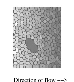
Figure 1:

Detail of a CPM simulation of a quasi-stationary flowing foam with a large bubble. The shading denotes bubble pressures, with darker shades denoting lower pressures.

Fig. 1 shows a detail of a simulation with a large bubble moving through smaller bubbles. The shades denote the pressure inside each bubble, darker shades denoting lower pressures. The bubbles move from left to right. Our lattice geometry is rectangular (usually 1000 X 200 sites) with open boundary conditions at the short sides, like a H-S experiment. We nucleate bubbles at a steady rate at one short end (the head end) and remove them at the opposite short end (the tail end).

All the bubbles, except the large bubble, nucleate at a fraction of their target area (large pressure). As they enter the lattice, they gradually expand, generating an excess pressure at the head end. As the bubbles move from left to right, they expand and their pressure decreases. When a bubble contacts the tail end of the lattice, we set its area constraint to zero so that it disappears smoothly at near zero pressure. Pressure differences between bubbles induce boundary movement with a velocity proportional to the applied force jiang . This method of bubble creation and disappearance corresponds closely to the experiments which generate bubbles continuously at one end of the channel and allow them to exit at near-atmospheric pressure at the opposite end. Thus simulation and experiment both have a constant bubble-flux boundary condition at the head end and an absorbing boundary condition at the tail end. As we mentioned earlier, the absence of a simple relationship between the mobility of the bubbles and $J$ and $\lambda$ is a limitation of both the CPM and experiments.

Our simulations have $J=5$ and $\lambda=3$ and run at zero temperature. The small bubbles target area is usually 625 lattice sites. We create a single large bubble of diameter $D$ at the first time step at a random position along the head end. We nucleate small bubbles every 50 MCS with the initial sizes between 4 and 481 pixels. Varying the nucleation size of the bubbles at the head end changes the pressure gradient, which in turn changes the velocity of the flow. We also vary the large bubble size. If the large bubble radius is more than four times the small bubble radius, we use a larger lattice to avoid boundary effects. The small bubbles all have approximately the same velocity at any given time and we define the foam velocity as the average of the center-of-mass velocities of the small bubbles at a fixed time. For each case, we run multiple replicas with different random number generator seeds. As in refs. okuzono and jiang we define the total stored surface energy $\phi$ to be,

$$\phi=\sum_{i,j}(1-\delta_{i,j}).$$ (8)

The average stress tensor $\sigma$, as ref. okuzono points out, relates directly to $\phi$. $\phi=Tr(\sigma)$. We scale out differences due to initial conditions by using $\phi(t)\over\phi(0)$, where $\phi(0)$ is the value of $\phi$ at the start of the simulation. The applied strain rate is very high initially, then falls sharply to a low constant value, after which the applied strain is proportional to time and the energy vs time curve becomes equivalent to the energy vs applied strain curve. We call the flow quasistationary when any drift in the total energy is less than 2% of the average energy over 1000 MCS and the bubble velocity changes by less than 10 % of the average velocity over 1000 MCS. We make all measurements in the quasistationary state. Since bubbles we introduce and eliminate continuously we are never in a static state equilibrium. The finite H-S cell and pressure drop along it means that bubble velocity varies down the cell length.

III Results

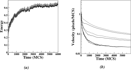
Figure 2:

(a) Equilibration of the stored surface energy of a simulated flowing foam containing a large bubble with small bubbles nucleating every 50 MCS.

(b) Equilibration of bubble velocities in a simulated flowing foam: large bubbledashed lines, small bubblessolid lines. The three pairs of curves are for different nucleation sizes of the small bubbles. The lowest curve corresponds to an initial nucleation size of 481 pixels and the higher curves to nucleation sizes of 156 and 25 pixels respectively.

Fig 2 (a) plots $\phi$ as a function of time and fig 2 (b) plots the velocity of large and small bubbles as a function of time. For slow flows, the small and large bubbles flow with the same velocity as a solid. Above a critical velocity the bubbles’ velocities depend on their sizes, e.g., our simulations the critical velocity is 0.014 pixels/MCS when the radius of the large bubble is twice that of the small bubbles. We plot the difference in velocity between the large bubble and the foam ($v_{L}-v_{f}$) vs the velocity of the foam $v_{f}$ for different large-bubble sizes $D$, scaling the velocity difference by $r=D/d$, where the diameter of the small bubbles $d$ is constant. Fig. 3 shows our results. We checked that $v_{c}$ was independant of $d$ by running simulations with a small bubble target area, $A_{n}=400$ pixels. We examined the cases $r=2,3,3.5$ and $4$. Since very large bubbles tend to wobble and break into smaller bubbles, we analyzed only simulations in which the large bubble traversed the H-S cell without breaking. We find excellent agreement between our data and the theoretical form of Cantat and Delanney cantat ;

$${(v_{L}-v_{f})\over v_{f}(D/d)}={-A\over v_{f}}\times{1\over Bln(1-{A\over v_{f}})},$$ (9)

where $(v_{L}-v_{f})$ is the difference between the large bubble velocity and the foam velocity and $A$ and $B$ are fitting parameters. The fitting value of the critical velocity $A=0.013$ pixels/MCS, $B=8.66$ is a dimensionless parameter which scales the velocity. The asymptotic standard error for both parameters is less than $5\%$.

Figure 3:

Difference between large bubble velocity $v_{L}$ and average foam velocity, rescaled by $rv_{f}$, vs $v_{f}$ for different large-bubble sizes, on a semilog scale. The symbols on the graph correspond to different values of $r$.

The theoretical critical velocity is cantat :

$$v_{c}={\gamma h\over\eta D},$$ (10)

where $h$ is the thickness of the H-S cell. Taking $h$ to be the small bubble size, we obtain $v_{c}$ from the values of $\gamma$ and $\eta$ obtained from our simulations. We obtain $\eta$ by measuring the relation between the effective pressure along the channel and the foam velocity and $\gamma$ from the size and pressure of the small bubbles. We find $v_{c}=0.014$ pixels/MCS, agreeing with the value which we obtained in the previous paragraph.

We can also calculate an analog of the Deborah number ($N_{D}$) for our simulated bubble motion, the product of the shear strain rate and the event timescale durian . The event timescale $\tau$ is the timescale of a T1, while the shear strain rate is the ratio of the velocity difference to the lengthscale (which in our case is the size of the small bubbles). So,

$$N_{D}={(v_{L}-v_{f})\tau\over d}.$$ (11)

Our small bubble size is usually 25 pixels, while $\tau$ is approximately $20$ MCS so $N_{D}$ is between $10^{-2}$ and $10^{-1}$ for most of our simulations. Our maximum $N_{D}$ is $0.08$.

IV Conclusions.

We have shown that we can use the CPM to study the flow of a large bubble embedded in a monodisperse foam. For small velocities, all the bubbles in the foam flow at the same velocity. Above a critical velocity, the velocities of the bubbles vary with their sizes. The critical velocity in our detailed simulations of a large bubble twice the size of the small bubbles matches very well with the critical velocity we obtain by fitting our simulation results for bubbles of various sizes to the analytical equation of Cantat and Delennay cantat , and with the critical velocity we deduce theoretically from the effective viscosity and surface tension of the simulated foam.

We have also checked that in a polydisperse foam, above a critical velocity different-size bubbles travel at different velocities, the large bubbles traveling faster. The dimensional form of the definition of the critical velocity suggests that bubbles of different sizes should have different critical velocities, however we have not been able to verify this dependance in a simulated polydisperse foam because the very large scatter in the velocity difference prevents us from identifying the critical velocities. Experiments by Park and Durian revealed fingering instabilities in radial H-S cells park which may relate to the viscous instability in rectangular H-S cells. However the aspect ratios of these experiments are very different from those in our simulations, so direct comparison is difficult.

Acknowledgements: We acknowledge the use of AVIDD, the distributed computing facility at Indiana University Bloomington to run our simulations. We thank Debasis Dan, Ariel Balter, Lenhilson Coutinho, Roeland Merks and Julio Espinoza Ortiz for discussions, suggestions and comments. We also thank Isabelle Cantat for supplying the preprints which we cite in this paper and discussing the details of her experiments and simulations. We also acknowledge support from NSF grant IBN-0083653, NASA grant NAG2-1619, an IBM Innovation Institute award, an Indiana University Pervasive Technologies Laboratory Fellowship and the Biocomplexity Institute.

References

- (1) J. C. Slattery, A. I. Ch. E. Journal, 25, 2. 283 (1999)
- (2) A. M. Kraynik, Annu. Rev. Fluid Mech. 20, 325 (1988).
- (3) D. Weaire and S. Hutzler, The Physics of Foams, (Oxford University Press, Oxford, 2000).
- (4) S. Cox, D. Weaire, and J. A. Glazier, Rheol. Acta 43, 442 (2004).
- (5) A. D. Gopal and D. J. Durian, Phys. Rev. Lett. 75, 2610 (1995).
- (6) D. Weaire and N. Rivier, Contemp. Phys. 25, 55 (1984).
- (7) H. M. Princen, J. Colloid Interface Sci. 91, 160 (1983).
- (8) S. A. Khan and R. C. Armstrong, J. Non-Newtonian Fluid Mech. 22, 1 (1986); 25, 61 (1987).
- (9) D. A. Reinelt and A. M. Kraynik, J. Fluid Mech. 215, 431 (1990).
- (10) K. Kawasaki, T. Nagai, and K. Nakashima, Philos. Mag. B 60, 399 (1989); K. Nakashima, T. Nagai, and K. Kawasaki, J. Stat. Phys. 57, 759 (1989).
- (11) T. Okuzono and K. Kawasaki, Phys. Rev. E 51, 1246 (1995).
- (12) D. J. Durian, Phys. Rev. Lett. 75, 4780 (1995); D. J. Durian, Phys. Rev. E 55, 1739 (1997).
- (13) D. Weaire, F. Bolton, T. Herdtle and H. Aref, Philos. Mag. Lett. 66, 293 (1992).
- (14) J. A. Glazier, M. P. Anderson and G. S. Grest, Philos. Mag. B 62, 615 (1990); J. A. Glazier, Phys. Rev. Lett. 70, 2170 (1993); Y. Jiang and J. A. Glazier, Philos. Mag. Lett. 74, 119 (1996); F. Graner and J. A. Glazier, Phys. Rev. Lett. 69, 2013 (1992); J. A. Glazier and F. Graner, Phys. Rev. E 47, 2128 (1993).
- (15) Y. Jiang, P. J. Swart, A. Saxena, M. Asipauskas and J. A. Glazier, Phys. Rev. E 59, 5819 (1999).
- (16) C. Z. Van Doorn, J. Appl. Phys. 46, 3738 (1975).
- (17) C. A. Hieber, in Injection and Compression Molding Fundamentals, edited by A. I. Isayev, (Marcel Dekker, New York, 1987).
- (18) O. Lordereau, Ph.D thesis, Universite de Rennes, 2002.
- (19) I. Cantat and R. Delannay, Phys. Rev. E 67, 031501 (2003) I. Cantat and R. Delannay, preprint, (2004).
- (20) J. C. Earnshaw and M. Wilson, J. Phys. Condens. Matter. 7, L49 (1995).
- (21) B. Dollet, F. Elias, C. Quilliet, A. Huillier, M. Aubouy, and F. Graner, Colloids and Surfaces A, 263, 101 (2005).
- (22) B. Dollet, F. Elias, C. Quilliet, C. Raufaste, M. Aubouy and F. Graner, Phys. Rev. E 71, 031403 (2005).
- (23) N. Kern, D. Weaire, A. Martin, S. Hutzler, and S. J. Cox, Phys. Rev. E 70,041411 (2004).
- (24) I. Cantat, N. Kern and R. Delannay, Europhys. Lett., 65 (5), 726 (2004).
- (25) S. S. Park and D. J. Durian, Phys. Rev. Lett.72, 3347 (1994)