Orbital fluctuations and strong correlations in quantum dots

Abstract

In this lecture note we focus our attention to quantum dot systems where exotic strongly correlated behavior develops due to the presence of orbital or charge degrees of freedom. After giving a concise overview of the theory of transport and Kondo effect through a single electron transistor, we discuss how $SU(4)$ Kondo effect develops in dots having orbitally degenerate states and in double dot systems, and then study the singlet-triplet transition in lateral quantum dots. Charge fluctuations and Matveev’s mapping to the two-channel Kondo model in the vicinity of charge degeneracy point are also discussed.

I Introduction

Although no rigorous definition exists, we typically call a ’quantum dot’ a small artificial structure containing conduction electrons, and weakly coupled to the rest of the world. There is a variety of ways to produce these structures: Maybe the most common technique to do this is by defining a typically $\mu{\rm m}$-size region by shaping a two-dimensional electron gas using gate electrodes placed on the top of a semiconductor heterostructure or by etching (see, e.g., Refs. David, ; TaruchaST, ; review, ). In Fig. 1 we show the top view of such a single electron transistor (SET) that has been first used to detect the Kondo effect in such a structure.David Beside semiconductor technologies, quantum dots can also be built from metallic grains Devoret ; Ralph_metallic , and more recently it became possible to integrate even real molecules into electronic circuitsmolecular_SET . The common feature of all these devices is that Coulomb correlations play an essential role in them, and induce Coulomb blockadeCoulomb_blockade and Kondo effect.David ; Leo ; Kondo_dot

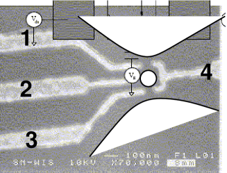
Figure 1: Top view of the SET used by David Goldhaber-Gordon and his collaborators to first observe the Kondo effect in a quantum dot, from Ref. David, : The white areas indicate regions where conduction electrons are present. The quantum dot is at the central region (white circle). The various electrodes (1-4) have been used to define the dot and the junctions.

In the present paper (which has been prepared as a lecture note) we shall not attempt to give a complete overview of this enormous field. Instead, we shall first give a concise introduction into the basic properties of these devices, and then focus our attention to some exotic strongly correlated states associated with orbital and charge degrees of freedom that appear in them.

There is two essential energy scales that characterize an isolated quantum dot: One of them is the charging energy, $E_{C}$, the typical cost of putting an extra electron on the device. The other is the typical separation of single particle energies, also called level spacing, $\Delta$. Typically $\Delta\ll E_{C}$, but for very small structures (e.g. in the extreme case of a molecule) these two energy scales can be of the same order of magnitude. While the charging energy $E_{C}$ is usually of the order of $e^{2}/L$ with $L$ the characteristic size of the device, the level spacing $\Delta$ depends very much on the material and dimensionality of the dot: it is typically very small in mesoscopic metallic grains, where it roughly scales as $\Delta\sim E_{F}/(k_{F}L)^{3}$, and becomes of the order of one Kelvin only for nanoscale structures with $L\sim 20\AA$. For two-dimensional semiconductor structures, on the other hand, both $k_{F}$ and the Fermi energy are much smaller and since $\Delta$ scales as $\Delta\sim E_{F}/(k_{F}L)^{2}$, in these structures $\Delta$ becomes of the order of a Kelvin typically for $L\sim 0.1\mu{\rm m}$.

Coulomb correlations may become only important if the measurement temperature is less than the charging energy, $T<E_{C}$. Clearly, this criterion can be only satisfied with our current cooling technology if $E_{C}$ is in the range of a few Kelvins, i.e. the size of the system is in the $\mu{\rm m}$ range or below. The behavior of a quantum dot is also very different in the regimes $T>\Delta$ and $T<\Delta$: while in the former regime electron-hole excitations on the dot are important, for $T<\Delta$ these excitations do not play an essential role.

Beside the difference in the typical energy scales $E_{C}$ and $\Delta$, there is also a difference in the way semiconducting and metallic devices are usually connected. Although metallic particles can also be contacted through single or few mode contacts using e.g. STM tips, these grains are typically connected through multichannel leads with contact sizes much larger than the Fermi wavelength $\lambda_{F}$. Lateral semiconducting devices are, on the other hand, usually contacted through few or single mode contacts (though e.g. vertical dots are connected through a large contact area and thus many channels). While these details can be important for some phenomena,Schoen ; Wilhelm the behavior of all these devices is very similar in many respects. In the following, we shall therefore mainly focus on lateral quantum dots with single mode contacts.

This lecture is organized as follows: First, in Section II we shall discuss the phenomenon of Coulomb blockade and the basic Hamiltonians that are used to describe quantum dots. In Section III we discuss how the Coulomb blockade is lifted by the formation of a strongly correlated Kondo state at very low temperatures, $T\ll\Delta$. In Section IV we shall study more exotic strongly correlated states that appear due to orbital degrees of freedom, the $SU(4)$ Kondo state, and the so-called singlet-triplet transition. Section V is devoted to the analysis of the Coulomb blockade staircase in the vicinity of the degeneracy points, where strong charge fluctuations are present.

II Coulomb blockade

In almost all systems discussed in the introduction we can describe the isolated dot by the following second quantized Hamiltonian

$$H_{\rm dot}=\sum_{j,\sigma}\epsilon_{j}\;d^{\dagger}_{j\sigma}d_{j\sigma}+H_{\rm int}+H_{\rm gate}\;,$$ (1)

where the second term describes interactions between the conduction electrons on the island, and the effects of various gate voltages are accounted for by the last term. The operator $d^{\dagger}_{j\sigma}$ creates a conduction electron in a single particle state $\varphi_{j}$ with spin $\sigma$ on the dot.

Fortunately, the terms $H_{C}=H_{\rm int}+H_{\rm gate}$ can be replaced in most cases to a very good accuracy by a simple classical interaction term Aleiner

$$H_{C}={e^{2}\over 2C}\left(n_{\rm dot}-{V_{g}C_{g}\over e}\right)^{2}\;,$$ (2)

where $C$ denotes the total capacitance of the dot, $C_{g}$ is the gate capacitance, $e$ is the electron’s charge, $V_{g}$ stands for the gate voltage (roughly proportional to the voltage on electrode ’2’ in Fig. 1), and $n_{\rm dot}=\sum_{j,\sigma}:d^{\dagger}_{j\sigma}d_{j\sigma}$ is the number of extra electrons on the dot. This simple form can be derived by estimating the Coulomb integrals for a chaotic dot Aleiner , however, it also follows from the phenomenon of screening in a metallic particle. We outline this rather instructive derivation of Eq. (2) within the Hartree approximation in Appendix A. Clearly, the dimensionless gate voltage $N_{g}={V_{g}C_{g}/e}$ sets the number of electrons on the dot, $\langle n_{\rm dot}\rangle\approx N_{g}$.

The single particle levels $\epsilon_{j}$ above are random but correlated: The distribution of these levels for typical (i.e. large and chaotic) islands is given with a good accuracy by random matrix theory,RandomMatrix which predicts among others that the separation $s$ between two neighboring states displays a universal distribution,

$$P(s)={1\over\Delta}p\left({s/\Delta}\right)\;,$$ (3)

with $\Delta$ the average level spacing between two neighboring levels. For small separations, energy levels repel each-other and $p$ vanishes as $p\left({s\over\Delta}\right)\sim\left({s\over\Delta}\right)^{\beta}$, where the exponent is $\beta=1,2$ or $4$, depending on the symmetry of the Hamiltonian (orthogonal, unitary, and simplectic, respectively). In some special cases cross-overs between various universality classes can also occur,and in some cases level repulsion may be even absent for dots with special symmetry properties.

Figure 2: Excitation spectrum of an island. Lines represent eigenenergies of the island. Charging excitations typically need an energy $\sim E_{C}$ while internal electron-hole and spin excitations cost an energy $\Delta\ll E_{C}$.

The spectrum of an isolated dot described by Eqs. (1) and (2) is sketched in Fig. 2. As we already mentioned, for typical parameters and relatively large lateral dots or metallic islands, the charging energy is much larger than the level spacing, $E_{C}\gg\Delta$. Accordingly, internal electron-hole excitations cost much smaller energy than charge excitations of the dot. For dot sizes in the $0.1\mu{\rm m}$ range the capacitance $C$ can be small enough so that the charging energy $E_{C}=e^{2}/2C$ associated with putting an extra electron on the dot can safely be in the ${\rm meV}$ range. Therefore, unless $N_{g}={V_{g}C_{g}\over e}$ is a half-integer, it costs a finite energy to charge the device, and therefore the number of electrons on the dot becomes quantized at low enough temperatures, $T\ll E_{C}$, and a Coulomb blockade develops - provided that quantum fluctuations induced by coupling the dot to leads are not very strong.

Let us now consider a quantum dot that is weakly tunnel-coupled to leads, ’weak coupling’ in this context meaning that the conductance between the island and the leads is less than the quantum conductance, $G_{Q}\equiv 2e^{2}/h$. In the particular case of a lateral quantum dot this condition is satisfied when the last conduction electron channel is being pinched off. If the lead-dot conductance is much larger than $G_{Q}$ then the Coulomb blockade is lifted by quantum fluctuations (see also Section V). In the absence of tunneling processes, the charge on the dot would change in sudden steps at $T=0$ temperature (see Fig. 3). However, in the vicinity of the jumps, where $N_{g}={V_{g}C_{g}\over e}$ is a half-integer, two charging states of the island become almost degenerate. Therefore quantum tunneling to the leads induces quantum fluctuations between these two charging states, smears out the steps, and eventually completely suppresses the steps only leaving some small oscillations on the top of a linear $\langle n_{\rm dot}\rangle(V_{g})$ dependence.lifting_blockade At a finite temperature $T\neq 0$, thermal fluctuations play a similar role, and the charging steps are also washed out if $T\gg E_{C}$.

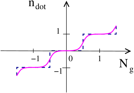
Figure 3: The number of electrons on a quantum dot as a function of the dimensionless gate voltage. The sudden jumps of an isolated dot become smeared out due to quantum fluctuation as soon as we couple the dot to leads.

Charge quantization is also reflected in the transport properties of the dot. To study transport through a quantum dot, one typically builds a single electron transistor (SET) by attaching the dot to two leads, as shown in Figs. 1 and 4. Let us first assume that the conductances $G_{L}$ and $G_{R}$ between the dot and the lead on the left / right are small compared to $G_{Q}$ and that quantum fluctuations are small. In this limit we can describe charge fluctuations on the dot by the following simple tunneling Hamiltonian:

$$\hat{V}=\sum_{j}\sum_{\epsilon}\Bigl{\{}t^{L}_{j}\;d^{\dagger}_{j\sigma}\psi_{L,\epsilon\sigma}+{\rm h.c.}\Bigr{\}}+``L\leftrightarrow R^{\prime\prime}\;,$$ (4)

where we assumed single mode contacts. The fields $\psi_{L,\epsilon\sigma}^{\dagger}$ and $\psi_{R,\epsilon\sigma}^{\dagger}$ denote the creation operators of conduction electrons of energy $\epsilon$ and spin $\sigma$ in the left and right leads, respectively, and are normalized to satisfy the anticommutation relations $\{\psi_{L/R,\epsilon\sigma}^{\dagger},\psi_{L/R,\epsilon^{\prime}\sigma^{\prime}}\}=\delta_{\sigma\sigma^{\prime}}\delta_{\epsilon\epsilon^{\prime}}$. Note that the tunneling matrix elements $t^{L}_{j}$ and $t^{R}_{j}$ fluctuate from level to level since they depend on the amplitude of the wave function $\varphi_{j}$ at the tunneling position. Using a simple Boltzmann equation approach one then finds that for $T<E_{C}$ the linear conductance of the SET has peaks whenever two charge states of the dot are degenerate and $N_{g}$ is a half-integer. In the regime, $\Delta\ll T\ll E_{C}$, in particular, one finds that peak

$$G(T)\approx{1\over 2}{G_{L}G_{R}\over G_{L}+G_{R}}{\Delta E/T\over{\rm sinh}(\Delta E/T)}\;,$$ (5)

where $\Delta E$ is the energy difference between the two charging states of the dot, and $G_{L/R}=(8\pi^{2}e^{2}/h)\;\varrho_{\rm dot}\;\varrho_{L/R}\;\langle|t^{L/R}_{j}|^{2}\rangle_{j}$ is the tunnel conductance of the two junctions, with $\varrho_{\rm dot}$ and $\varrho_{L/R}$ the density of states on the dot and the leads. Note that even for perfect charge degeneracy, $\Delta E=0$, the resistance of the SET is twice as large as the sum of the two junction resistances due to Coulomb correlations. As we decrease the temperature, the conductance peaks become sharper and sharper, while the conductance between the peaks decreases exponentially, and the Coulomb blockade develops. This simple Boltzmann equation picture, however, breaks down at somewhat lower temperatures, where higher order processes and quantum fluctuations become important. These quantum fluctuations may even completely lift the Coulomb blockade and result in a perfect conductance at low temperatures as we shall explain in the next section.

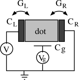
Fig.a

Fig.b

Figure 4: (a) Sketch of a single electron transistor. (b) Conductance of the SET as a function of gate voltage for $E_{C}\ll T\ll\Delta$. At the degeneracy points Coulomb blockade is lifted and transport is allowed through the single electron transistor.

Let us first study the conductance of the SET in the regime where the difference $\Delta E$ between the energy of the two charging states considered is much larger than the temperature. It turns out that the range of validity of Eq. (5) describing an activated behavior is rather small for typical parameters, and the conductance is dominated by second order virtual processes as soon as we lower the temperature much below $\Delta E$. From the point of view of these second order processes two regimes must be distinguished: In the regime $\Delta\ll T\ll E_{C}$ the leading term to the conductance comes from elastic and inelastic co-tunneling processes shown in Fig. 5:cotunneling In the inelastic co-tunneling process a conduction electron jumps into the dot from one lead and another electron jumps out of the dot to the other lead in a second order virtual process, leaving behind (or absorbing) an electron-hole excitation on the dot, while in an elastic co-tunneling it is the same electron that jumps out. Inelastic co-tunneling gives a conductance $G_{\rm inel}\sim G_{L}G_{R}(T/E_{C})^{2}/(e^{2}/h)$, and is thus clearly suppressed as the temperature decreases,cotunneling while elastic co-tunneling results in a small temperature independent residual conductance, $G_{\rm el}\sim G_{L}G_{R}(\Delta/E_{C})/(e^{2}/h)$ even at $T=0$ temperature.cotunneling

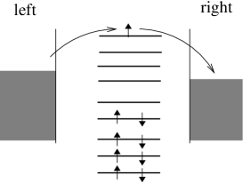
Fig.a

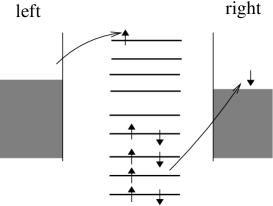
Fig.b

Figure 5: Elastic (a) and inelastic (b) co-tunneling processes. Inelastic co-tunneling processes give a conductance $\sim T^{2}$ while elastic co-tunneling gives a finite conductance as $T\to 0$.

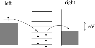
Figure 6: Exchange process leading to the enhancement of the conductance as $T\to 0$.

III Kondo effect

For $T\ll\Delta\ll E_{C}$ inelastic co-tunneling processes are not allowed, and the properties of the SET depend essentially on the number of electrons on the dot. The ground state of the isolated dot must be spin degenerate if there is an odd number of electrons on the dot, while it is usually non-degenerate, if the number of electrons on the dot is even. In the latter case nothing special happens: quantum fluctuations due to coupling to the leads produce just a residual conductance as $T\to 0$. If, however, the number of the electrons on the dot is odd, then the ground state has a spin degeneracy, which can give rise to the Kondo effect discussed below. In this case, exchange processes shown in Fig. 6 give a contribution to the conductance. As we lower the temperature, the effective amplitude of these processes increases due to the Kondo effect, and ultimately gives a conductance that can be as large as the quantum conductance $G_{Q}=2e^{2}/h$ at $T=0$ temperature.Leo This strong enhancement is due to strong quantum fluctuations of the spin of the dot, and the formation of a strongly correlated Kondo state. The typical temperature dependence of the conductance for $N_{g}$ odd is shown in Fig. 7.

Figure 7: (a) Linear conductance of the SET for $T_{K}\ll T\ll E_{C}$ (dashed line) and $T\to 0$ (solid line). (b) Temperature dependence of the conductance of a symmetrical SET for an odd number of electrons on the dot (continuous line) and for an even number of electrons with non-degenerate ground state (dashed line).

To understand why the conductance of the dot becomes large, let us keep only the last, singly occupied level that gives rise to the Kondo effect, $d_{j\sigma}\to d_{\sigma}$, $\epsilon_{j}\to\epsilon_{d}$, and write the Hamiltonian of the dot as

$$H = \sum_{\sigma}\epsilon_{d}\;d^{\dagger}_{\sigma}d_{\sigma}+H_{C}$$

$$+ \sum_{\sigma}\sum_{\mu=L,R}\int{d\epsilon}\;\epsilon\;\psi_{\mu,\sigma}^{\dagger}(\epsilon)\psi_{\mu,\sigma}(\epsilon)$$

$$+ \int d\epsilon\;\Bigl{\{}t^{L}\varrho_{L}^{1/2}\;(d^{\dagger}_{\sigma}\psi_{L,\sigma}(\epsilon)+{\rm h.c.})+``L\leftrightarrow R^{\prime\prime}\Bigr{\}}\;,$$

where we introduced the fields, $\psi_{L,\sigma}(\epsilon)\equiv\varrho_{L/R}^{1/2}\;\psi_{L/R,\epsilon\sigma}$. For the sake of simplicity, let us assume that $t^{R}\varrho_{L}^{1/2}=t^{L}\varrho_{R}^{1/2}$. If we then make a unitary transformation and introduce the even and odd field operators,

$$\psi_{\pm}\equiv{\psi_{R}\pm\psi_{L}\over\sqrt{2}}\;,$$ (7)

then obviously the odd combination $\psi_{-}$ fully decouples from the dot, and the tunneling part of the Hamiltonian can be written as

$$\hat{V}=\tilde{t}\int d\epsilon\;(d^{\dagger}_{\sigma}\psi_{+,\sigma}(\epsilon)+{\rm h.c.})\;,$$ (8)

where $\tilde{t}=\sqrt{2}\;t^{R}\varrho_{R}^{1/2}$. One can now perform second order degenerate perturbation theory in $\hat{V}$ in the subspace $\sum_{\sigma}d^{\dagger}_{\sigma}d_{\sigma}=1$ to obtain the following effective exchange Hamiltonian:

$$H_{\rm eff} = \sum_{\sigma}\sum_{\epsilon}\;\epsilon\;\psi_{+,\sigma}^{\dagger}(\epsilon)\psi_{+,\sigma}(\epsilon)$$

$$+ {J\over 2}{\vec{S}}\;\sum_{\sigma,\sigma^{\prime}}\int\int d\epsilon\;d\epsilon^{\prime}\psi_{+\sigma}^{\dagger}(\epsilon)\vec{\sigma}_{\sigma\sigma^{\prime}}\psi_{+\sigma^{\prime}}(\epsilon^{\prime})\;,$$

where $\vec{S}={1\over 2}(d^{\dagger}\vec{\sigma}d)$ is the spin of the dot, and $J\sim\tilde{t}^{2}/E_{C}$ is a dimensionless antiferromagnetic exchange coupling. Thus electrons in the even channel $\psi_{+}$ couple antiferromagnetically to the spin on the partially occupied $d$-level, and try to screen it to get rid of the residual entropy associated with it.

Written in the original basis, Eq. (III) contains terms $\sim J{\vec{S}}\psi_{R}^{\dagger}(\epsilon)\vec{\sigma}\psi_{L}(\epsilon^{\prime})$, which allow for charge transfer from one side of the dot to the other side, and in leading order these terms give a conductance $\sim J^{2}$. However, higher order terms in $J$ turn out to give logarithmically divergent contributions,

$$G\sim{e^{2}\over h}\Bigl{(}J^{2}+2\;J^{3}\;{\rm ln}(\Delta/T)+\dots\Bigr{)}\;.$$ (10)

As a result, the conductance of the device increases as we decrease the temperature and our perturbative approach breaks down at the so-called Kondo temperature,

$$T_{K}\approx\Delta e^{-1/J}\;.$$ (11)

One can try to get rid of the logarithmic singularity in Eq. (10) by summing up the most singular contributions in each order in $J$. This can be most easily done by performing a renormalization group calculation and replacing $J$ by its renormalized value in the perturbative expression, $G\sim{e^{2}\over h}J^{2}$.RG However, this procedure does not cure the problem and gives a conductance that still diverges at $T=T_{K}$,

$$G\sim{e^{2}\over h}{1\over{\rm ln}^{2}(T/T_{K})}\;.$$ (12)

The meaning of the energy scale $T_{K}$ is that below this temperature scale the effective exchange coupling becomes large and a conduction electron spin is tied antiferromagnetically to the spin of the dot to form a singlet (see Fig. 8).

Figure 8: Conduction electrons in the even channel screen the impurity spin.

It is not difficult to show that then for $t^{L}\varrho_{L}^{1/2}=t^{R}\varrho_{R}^{1/2}$ the SET must have perfect conductance at $T=0$ temperature. To show this, let us apply the Friedel sum rule,Hewson ; Friedel_Kondo that relates the number $N_{\rm bound}$ of electrons bound to the impurity and the phase shifts $\delta$ of the electrons $\psi_{+}$, as

$$N_{\rm bound}=2{\delta\over\pi}\;,$$ (13)

where the factor $2$ is due to the spin. This relation implies that in the even channel conduction electrons acquire a phase shift $\delta=\pi/2$, and correspondingly, $\psi_{+}\to e^{2i\delta}\psi_{+}=-\psi_{+}$ in course of a scattering process at $T=0$ temperature. Going back to the original left-right basis, this implies that left and right electrons scatter as

$$\psi_{L}\to-\psi_{R}\;,\phantom{nnn}\psi_{R}\to-\psi_{L}\;.$$ (14)

In other words, an electron coming from the left is transmitted to the right without any backscattering, and thus the quantum dot has a perfect conductance, $2e^{2}/h$.

We remark here that only a symmetrical device can have a perfect transmission, and only if the the number of electrons on the $d$-level is approximately one, $\langle n_{d}\rangle\approx 1$. All the considerations above can be easily generalized to the case $t^{L}\varrho_{L}^{1/2}\neq t^{R}\varrho_{R}^{1/2}$, and one obtains for the zero temperature conductance in the Kondo limit,

$$G(T\to 0)={2e^{2}\over h}{4\varrho_{L}t_{L}^{2}\;\varrho_{R}t_{R}^{2}\over(\varrho_{L}t_{L}^{2}+\varrho_{R}t_{R}^{2})^{2}}\;,$$ (15)

which is clearly less than $2e^{2}/h$ for non-symmetrical dots.

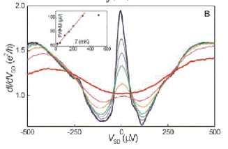
Figure 9: The Kondo resonance appears as a peak in the differential conductance of the SET (figure taken from Ref. Leo, ). At $T=0$ temperature the conductance approaches the quantum limit of the conductance, $2e^{2}/h$.

The phase shift $\delta=\pi/2$ also implies that there must be a resonance at the Fermi energy. In fact, this resonance is called the Kondo resonance, and can be directly seen in the differential conductance (related to the density of states as usual) of the single electron transistor shown in Fig. 9. This is a many-body resonance that develops at the Fermi energy (zero bias) as the temperature is cooled down below the Kondo temperature $T_{K}$.

The basic transport properties of the SET have been summarized in Fig. 7. Although we could get a fairly good analytical understanding of behavior of a SET, based on the simple considerations outlined above, it is rather difficult to obtain a quantitative description. In fact, to obtain a quantitative description extensive computations such as numerical renormalization group calculations are needed Theo . A valid and complete description of the out of equilibrium physics of a SET is still missing.Meir ; Achim ; Piers ; Schiller

IV Orbital degeneracy and correlations in quantum dots

In the previous section we sketched the generic behavior of a quantum dot, and assumed that the separation of the last, partially occupied level is by an energy distance $\sim\Delta\gg T$ separated from all other single particle levels of the dot. This is, however, not always true. In the case of a symmetrical arrangement like the one shown in Fig. 10, e.g., some of the states of the dot are orbitally degenerate by symmetry,Sasaki ; triangle while in some other cases almost degenerate orbitals may show up just by accident.vanderWiel ; KoganST This orbital degeneracy can play a very important role when we fill up these degenerate (or almost degenerate) levels, and leads to such phenomena as the SU(4) Kondo state triangle ; su4 or eventually the singlet-triplet transition.vanderWiel ; Sasaki ; KoganST

Figure 10: Arrangement with triangular symmetry and the structure of the four-fold degenerate ground state of the isolated triangular dot.

SU(4) physics and triangular dots

Let us first discuss what happens if we have just a single electron on an orbitally degenerate level. The presence of the orbital degeneracy leads to an unusual state of (approximate) SU(4) symmetry in this case, where spin and charge degrees of freedom are entangled. This SU(4) state has been proposed first theoretically to appear in double dot systems and quantum dots with triangular symmetry in Refs. su4, and triangle, . However, while there is no unambiguous experimental evidence of an SU(4) Kondo effect in double dot devices,Weis the SU(4) state has been recently observed in vertical dots of cylindrical symmetrySasaki2 as well as in carbon nanotube single electron transistors.Herrero In both chases the degeneracy index is due to a chiral symmetry just as in Ref. triangle, . Other realizations of states with SU(4) symmetry have been also proposed later in more complicated systems,Pascalsu4 ; LaciPascalsu4 and also in the context of heavy fermions.Michelesu4

For the sake of concreteness, we shall focus here to the case of the triangular dot shown in Fig. 10. However, our discussions carry over with trivial modifications to the previously mentioned experimental systems in Refs. Sasaki2, and Herrero, . Let us first assume that we have two orbitally degenerate levels $|\pm\rangle$ that can be labeled by some chirality index $\tau=\pm$, and let us focus on the charging of this multiplet only. At the Hartree-Fock level, these levels of the isolated dot can be described by:

$$H_{\rm dot}=\sum_{\tau,\tau^{\prime},\sigma}d^{\dagger}_{\tau\sigma}(E_{\tau\tau^{\prime}}+\Delta E\;\delta_{\tau\tau^{\prime}})d_{\tau^{\prime}\sigma}-{J_{H}\over 2}{\vec{S}}^{\;2}$$

$$+{E_{C}\over 2}(n_{+}+n_{-})^{2}+{\tilde{E}_{C}\over 2}(n_{+}-n_{-})^{2}\;,$$ (16)

where $d^{\dagger}_{\tau\sigma}$ creates an electron on the dot within the degenerate multiplet with spin $\sigma$ and orbital label $\tau$. The energy shift $\Delta E$ above is proportional to the (symmetrically-applied) gate voltage and controls the charge on the dot, while $E_{\tau\tau^{\prime}}$ accounts for the splitting generated by deviations from perfect triangular symmetry ($\sum_{\tau}E_{\tau\tau}=0$). We denote the total number of electrons in state $\tau=\pm$ by $n_{\tau}\equiv\sum_{\sigma}d^{\dagger}_{\tau\sigma}d_{\tau\sigma}$, and ${\vec{S}}={1\over 2}\sum_{\tau,\sigma,\sigma^{\prime}}d^{\dagger}_{\tau\sigma}{\vec{\sigma}}_{\sigma\sigma^{\prime}}d_{\tau\sigma^{\prime}}$ is the total spin of the dot. The terms proportional to $E_{C}$ and ${\tilde{E}_{C}}$ are generated by the Hartree interaction, while that proportional to $J_{H}$ in Eq. (16) is the Hund’s rule coupling, generated by exchange. This term has no importance if there is only a single electron on the dot.

Figure 11: Structure of the Coulomb blockade peaks of the triangular dot. The multiplets are labeled by the corresponding irreducible representations. The arrows indicate the direction the peaks move when applying a Zeeman field.

Let us first consider the linear conductance. The currents $I_{j}$ between leads $j$ and the dot are related to the voltages $V_{j}$ applied on them by the conductance tensor,

$$I_{j}=\sum_{j^{\prime}}G_{jj^{\prime}}V_{j^{\prime}}\;,$$ (17)

which further simplifies to $G_{jj^{\prime}}={3\over 2}G\delta_{jj^{\prime}}-G/2$ for a symmetrical system. A schematic plot of the conductance $G$ as a function of $\Delta E$ is shown in Fig. 11. The arrangement of the four Coulomb blockade peaks associated to the fourfold degenerate $\Gamma_{3}$ state is symmetrical, and the height of the four peaks turns out to be numerically almost identical at high temperatures.triangle

The most interesting regime in Fig. 11 appears between the first two peaks. Here there is one electron on the dot, and correspondingly the ground state of the isolated dot is fourfold degenerate. Let us now tunnel couple the dots to conduction electrons in the three leads, $\psi_{j}$ ($j=1,2,3$). To simplify the Hamiltonian we first introduce new fields that transform with the same symmetry as the states $|\tau\rangle$,

$$\psi_{j}\to\psi_{\pm}\equiv{1\over\sqrt{3}}\sum_{j}e^{\pm i\;2\pi j/3}\psi_{j}\;.$$ (18)

With this notation the tunneling Hamiltonian of a perfectly symmetrical dot becomes

$$\hat{V}=t\sum_{\sigma,\tau}\int d\epsilon\;\Bigl{(}d_{\tau\sigma}^{\dagger}\psi_{\tau\sigma}(\epsilon)+h.c.\Bigr{)}\;.$$ (19)

To describe the fourfold degenerate ground state of the dot, we can introduce the spin and and orbital spin operators $\vec{S}$ and $\vec{T}$, with $S_{z}=\pm 1/2$ and $T_{z}=\pm 1/2$ corresponding to the states $\sigma=\pm$ and $\tau=\pm$. Likewise, we can introduce spin and orbital spin operators $\vec{\sigma}$ and $\vec{\tau}$ also for the conduction electrons, and then proceed as in the previous section to generate an effective Hamiltonian by performing second order perturbation theory in the tunneling $\hat{V}$, Eq. (19). The resulting interaction Hamiltonian is rather complex and contains all kinds of orbital and spin couplings of the type $\sim T^{+}\tau^{-}{\vec{S}}{\vec{\sigma}}$ or $\sim T^{z}\tau^{z}$.su4 ; triangle These terms are generated by processes like the one shown in Fig. 12, and clearly couple spin and orbital fluctuations to each-other.

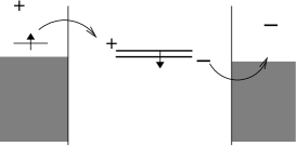
Figure 12: Example of a virtual process generating a coupling between the spin and the orbital spin.

Fortunately, a renormalization group analysis reveals that at low temperatures the various couplings become equal, and the Hamiltonian can be simply replaced by the following remarkably simple SU(4) symmetrical effective Hamiltonian (Coqblin-Schrieffer model),

$$H_{\rm eff}(T\to 0)=\tilde{J}\sum_{\alpha,\beta=1,..,4}\psi_{\alpha}^{\dagger}\psi_{\beta}\;|\beta\rangle\langle\alpha|\;,$$ (20)

where the index $\alpha$ labels the four combinations of possible spin and pseudospin indices, and the $|\alpha\rangle$’s denote the four states of the dot. The dynamical generation of this SU(4) symmetry can also be verified by solving the original complicated Hamiltonian by the powerful machinery of numerical renormalization group.Wilson ; su4 We remark here that the structure of the fixed point Hamiltonian, Eq. (20) is rather robust. Even if the system does not have a perfect triangular (or chiral) symmetry, the exchange part of the effective Hamiltonian at low temperatures will take the form Eq. (20), and the effect of imperfect symmetry only generates some splitting $E_{\tau\tau^{\prime}}$ for the orbitally degenerate levels and some small potential scattering.Mstate These terms, of course, break the SU(4) symmetry of Eq. (20), but represent only marginal perturbations, and do not influence the physical properties of the system in an esential way if they are small. In a similar way, the SU(4) symmetric fixed point discussed here may be relevant even for systems with (approximate) accidental degeneracy even if they do not have a perfect SU(4) symmetry.

Similar spin and orbital entangled states apparently also show up in molecular clusters, but there they may lead to the appearance of unusual non-Fermi liquid states.Crommie ; Cr3 ; Ingersent

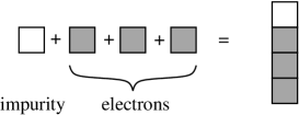
Figure 13: To screen the SU(4) spin of a triangular dot one needs three conduction electrons. The singlet formed corresponds to the Young tableau on the right, while the defining four-dimensional SU(4) representations are denoted by squares.

The Hamiltonian Eq. (20) is one of the exactly solvable models,WiegmannTsvelick and has been studied thoroughly before.CoqblinSchrieffer ; NozieresBlandin Just as in the Kondo problem studied in the previous section, the SU(4) spin of the dot is screened below the ’SU(4)’ Kondo temperature, $T_{K}^{(0)}$. However, to screen an SU(4) spin, one needs three conduction electrons, as shown in Fig. 13. As a result, the Friedel sum rule in the present case is modified to

$$3=\sum_{\sigma,\tau}{\delta_{\sigma\tau}\over\pi}=4{\delta\over\pi}\;,$$ (21)

corresponding to a phase shift $\delta=3\pi/4$ for the electrons $\psi_{\pm,\sigma}$.

The application of a magnetic field on the dot, $H\to H-B\;S^{z}$ clearly suppresses spin fluctuations.footnote_inplane However, it does not suppress orbital fluctuations, which still lead to a more conventional SU(2) Kondo effect, by replacing the spin in the original Kondo problem. The Kondo temperature $T_{K}^{\rm orb}$ of this orbital Kondo effect is, however, somewhat reduced compared to the SU(4) Kondo temperature $T_{K}^{(0)}$,triangle

$$T_{K}^{\rm orb}\sim{(T_{K}^{(0)})^{2}\over\Delta}\;.$$ (22)

The phase shifts in this case are simply $\delta_{\uparrow}\equiv\delta_{\pm,\uparrow}\approx\pi/2$, while $\delta_{\downarrow}\equiv\delta_{\pm,\downarrow}\approx 0$, just as for the original Kondo problem. The splitting of the two levels $\tau=\pm$ has a similar effect and drives the dot to a simple spin SU(2) state.

The zero-temperature phase shifts can be related to the transport properties of the device: From the $T=0$ phase shifts $\delta_{\tau\sigma}$ one can construct the conduction electrons’ scattering matrix in the original basis $\psi_{j}$ and compute all transport coefficients using the Landauer-Buttiker formula.Buttiker ; triangle ; Pustilnik The $T=0$ conductance $G$ turns out to be independent of the magnetic field, and both for the SU(4) and orbital Kondo states one finds the same value,

$$G(B)={8e^{2}\over 9h}\sum_{\sigma}\sin^{2}(\delta_{\sigma}(B))={8e^{2}\over 9h}\;.$$

The polarization of the current,

$$P={\sin^{2}(\delta_{\uparrow})-\sin^{2}(\delta_{\downarrow})\over\sin^{2}(\delta_{\uparrow})+\sin^{2}(\delta_{\downarrow})}\;,$$ (23)

however, does depend on the magnetic field and takes the values $P=0$ and $P=1$ in the SU(4) and orbital Kondo states, respectively. The phase shifts in Eq. (23) can be extracted with very high accuracy from the finite size spectrum computed via the numerical renormalization group procedure,Wilson ; su4 ; HofstetterZarand and the results (originally computed for the double dot system in Ref. su4, ) are shown in Fig. 14. Clearly, this device can be used as a spin filter: Applying a Zeeman field one can induce a large spin polarization at low temperatures while having a large $\sim e^{2}/h$ conductance through the device. A slightly modified version of this spin filter has indeed been realized in Ref. Herrero, , where two orbital states originating from different multiplets have been used to generate the orbital Kondo effect.

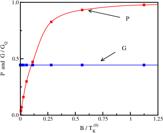
Figure 14: Spin polarization of the current through the triangular dot as a function of magnetic field.

To close the analysis of the SU(4) Kondo effect, let us shortly discuss how the SU(4) state emerges in capacitively coupled quantum dots, where it actually has been identified first. In this device, shown in Fig. 15, the capacitively coupled dots can be described by the following simple Hamiltonian

$$H_{\rm dot}={E_{C+}\over 2}(n_{+}-N_{g+})^{2}+{E_{C-}\over 2}(n_{-}-N_{g-})^{2}+{\tilde{E}}_{C}n_{+}n_{-}\;,$$ (24)

where the dimensionless gate voltages $N_{g\pm}$ set the number $n_{+}$ and $n_{-}$ of the electrons on the left and right dots, respectively. The last term is due to the capacitive coupling between the two dots, and it is essentially this term which is responsible for the SU(4) physics discussed. As shown in Fig. 15.b, in the parameter space of the two-dot regions appear, where the two states $(n_{+},n_{-})=(1,0)$ and $(n_{+},n_{-})=(0,1)$ are almost degenerate, while the states $(n_{+},n_{-})=(0,0)$ and $(n_{+},n_{-})=(1,1)$ are pushed to higher energies of order $\sim{\tilde{E}}_{C}$. In the simplest, however, most frequent case the states $(1,0)$ and $(0,1)$ have both spin $S=1/2$, associated with the extra electron on the dots. Therefore, in the regime above for temperatures below the charging energy $\tilde{E}_{C}$ and the level spacing $\Delta$ of the dots, the dynamics of the double dot is essentially restricted to the subspace $\{S^{z}=\pm 1/2;\;n_{+}-n_{-}=\pm 1\}$, and we can describe its charge fluctuations in terms of the orbital pseudospin $T^{z}\equiv(n_{+}-n_{-})/2=\pm\frac{1}{2}$. Coupling the two dot system to leads, we arrive at the very same Hamiltonian as for the triangular dots, although with very different parameters. Much of the previous discussions apply to this system as well which, in addition to being a good spin-filter, also exhibits a giant magneto-resistance.su4

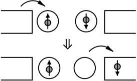
(a)

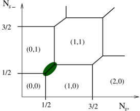
(b)

Figure 15: (a) A virtual process leading to entanglement between charge and spin fluctuations and the SU(4) Kondo state in the double dot device. (b) Charging states of the double dot device as a function of the dimensionless gate voltages $N_{g\pm}$. The colored region indicates the regime where the two states $(1,0)$ and $(0,1)$ are almost degenerate.

Singlet-triplet transition

So far we discussed the case where there is a single conduction electron on the degenerate levels. The regime between the two middle peaks in Fig. 11 where there is two electrons on the (almost) degenerate multiplet is, however, also extremely interesting.

In this regime the Hund’s rule coupling $J_{H}$ in Eq. (16) is very important. This coupling is typically smaller than the level spacing $\Delta$ in usual quantum dots. If, however, it is larger than the separation between the last occupied and first empty levels, $\delta\epsilon$, then it gives rise to a triplet ground state with $S=1$. In particular, such a spin $S=1$ state forms if one puts two electrons on the orbitally degenerate level of a symmetrical quantum dot discussed before,triangle ; Herrero but almost degenerate states may also occur in usual single electron transistors just by accident.vanderWiel Since in many cases one can shift the levels and thus tune $\delta\epsilon$ by an external magnetic fieldvanderWiel ; Herrero or simply by changing the shape of the dot by gate electrodes,KoganST one can actually drive a quantum dot from a triplet to a singlet state as illustrated in Fig. 16.

Figure 16: The state of a quantum dot changes from a triplet to a singlet as the separation $\delta\epsilon$ between the last occupied and first empty level increases.

While this transition has been first studied in vertical dots,Sasaki ; Pustilnik ; Eto here we shall focus on the usual lateral arrangement of Fig. 16 which has very different transport properties.vanderWiel ; real ; VBH ; HofstetterZarand For the sake of simplicity let us assume that we have a completely symmetrical device and that the two levels $|\pm\rangle$ participating in the formation of the triplet state are even and odd. In this case we can introduce the even and odd fields $\psi_{\pm}\equiv{(\psi_{R}\pm\psi_{L})/\sqrt{2}}$ by Eq. (7), which by symmetry only couple to the even and odd states, $|+\rangle$ and $|-\rangle$, respectively. The hybridization term in this case simply reads

$$\hat{V} = t_{+}\sum_{\sigma}\int d\epsilon\;\Bigl{(}d_{+\sigma}^{\dagger}\psi_{+\sigma}(\epsilon)+h.c.\Bigr{)}$$ (25)

$$+ t_{-}\sum_{\sigma}\int d\epsilon\;\Bigl{(}d_{-\sigma}^{\dagger}\psi_{-\sigma}(\epsilon)+h.c.\Bigr{)}\;.$$

To describe the isolated dot we can use the following simplified version of Eq. (16),

$$H_{\rm dot}=\sum_{\sigma}\Bigl{(}\epsilon_{+}d^{\dagger}_{+\sigma}d_{+\sigma}+\epsilon_{-}d^{\dagger}_{-\sigma}d_{-\sigma}\Bigr{)}$$

$$-{J_{H}\over 2}{\vec{S}}^{\;2}+{E_{C}\over 2}(n_{+}+n_{-})^{2}\;.$$ (26)

It is instructive to study the triplet state of the dot first, $\delta\epsilon\ll J_{H}$. Second order perturbation theory in Eq. (25) in this regime gives the following Hamiltonian replacing (III)

$$H_{\rm eff} = \sum_{\tau=\pm}\sum_{\sigma}\sum_{\epsilon}\;\epsilon\;\psi_{\tau,\sigma}^{\dagger}(\epsilon)\psi_{\tau,\sigma}(\epsilon)$$

$$+ {J_{+}\over 2}{\vec{S}}\;\sum_{\sigma,\sigma^{\prime}}\int\int d\epsilon\;d\epsilon^{\prime}\psi_{+\sigma}^{\dagger}(\epsilon)\vec{\sigma}_{\sigma\sigma^{\prime}}\psi_{+\sigma^{\prime}}(\epsilon^{\prime})$$

$$+ {J_{-}\over 2}{\vec{S}}\;\sum_{\sigma,\sigma^{\prime}}\int\int d\epsilon\;d\epsilon^{\prime}\psi_{-\sigma}^{\dagger}(\epsilon)\vec{\sigma}_{\sigma\sigma^{\prime}}\psi_{-\sigma^{\prime}}(\epsilon^{\prime})\;.$$

Clearly, the even and odd electrons couple with different exchange couplings $J_{\pm}$ to the spin. However, now $\vec{S}$ is a spin $S=1$ operator, and to screen it completely, one needs to bind two conduction electrons to it. This implies that an electron from both the even and the odd channels will be bound to the spin, and correspondingly two consecutive Kondo effects will take place at temperatures

$$T_{+}\approx\Delta\;e^{-1/J_{+}}\;\gg\;T_{-}\approx\Delta\;e^{-1/J_{-}}\;.$$ (28)

This also implies that the conductance at $T=0$ temperature must vanish in the Kondo limit by the following simple argument:real Again, we can use the Friedel sum rule to obtain the $T=0$ temperature phase shifts $\delta_{\pm}=\pi/2$ in both the even and odd channels. In the original left-right basis this implies that the lead electrons scatter as $\psi_{L/R}\to-\psi_{L/R}$, i.e., their wave function vanishes at the dot position (by Pauli principle), and $\psi_{L/R}$ are completely reflected.

It is a simple matter to express the $T=0$ temperature conductance in terms of the $T=0$ temperature phase shifts by means of the Landauer-Buttiker formula asButtiker

$$G={e^{2}\over h}\sum_{\sigma}\sin^{2}(\delta_{+,\sigma}-\delta_{-,\sigma})\;.$$ (29)

This formula immediately implies that the conductance as a function of a Zeeman field $B$ must be non-monotonic:real As we argued before, the conductance of the dot is small for $B=0$ at $T=0$ temperature. For $T_{-}\ll B\ll T_{+}$, however, the Kondo effect in the odd channel is suppressed and correspondingly the phase shifts in this channel are approximately given by $\delta_{-\uparrow}\approx\pi$ and $\delta_{-\downarrow}\approx 0$, while the phase shifts in the even channel are still $\delta_{-\sigma}\approx\pi/2$, and thus by Eq. (29) the conductance must be close to $2e^{2}/h$. For even larger magnetic fields, $B\gg T_{+},T_{-}$, the Kondo effect is killed in both channels, and correspondingly $\delta_{\pm\uparrow}\approx\pi$ and $\delta_{\pm\downarrow}\approx 0$, resulting in a small conductance again. The magnetic field dependence of the phase shifts obtained from a numerical renormalization group calculation and the corresponding conductance are shown in Fig. 17.HofstetterZarand By general arguments,real similar non-monotonic behavior must occur in the temperature- and bias-dependence of the conductance, as it has indeed been observed experimentally.real ; vanderWiel

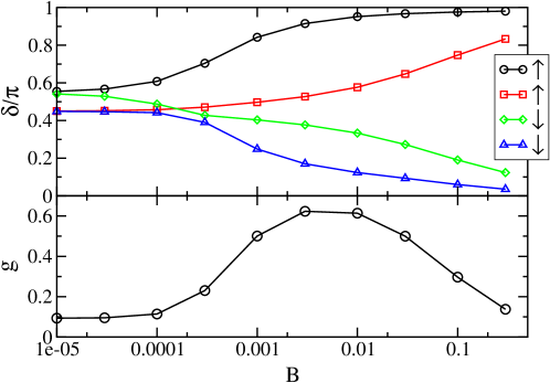
Figure 17: Phase shifts (top) and dip structure in the conductance as a function of Zeeman field $B$ on the triplet side of the transition at zero temperature, computed by the numerical renormalizaion group method (from Ref. HofstetterZarand, ).

Clearly, the $T=0$ temperature conductance must be also small on the singlet side of the transition, $\delta\epsilon\gg J_{H}$, where the dot is in a singlet state and no Kondo effect occurs. However, in the vicinity of the degeneracy point, $\delta\epsilon\approx J_{H}$, the triplet and the singlet states of the dot are almost degenerate, and quantum fluctuations between these four states generate another type of strongly correlated state with an increased Kondo temperature and a large conductance.vanderWiel ; HofstetterZarand ; real

To compute the full $T=0$ conductance as a function of $\delta\epsilon$ non-perturbative methods such as numerical renormalization group are needed.HofstetterZarand In the vicinity of the transition point the conductance goes up to $2e^{2}/h$, in perfect agreement with the experimental observations. While the non-monotonic behavior characteristic of the triplet state disappears in the vicinity of the transition, it reappears on the singlet side. However, there the size of the dip is not determined by the smaller Kondo scale, $T_{-}$, but rather by the excitation energy of the triplet, $\sim\delta\epsilon-J_{H}$.vanderWiel ; VBH ; HofstetterZarand Note that the transition between the triplet and singlet states is smooth and the singlet-triplet transition is rather a cross-over than a phase transition in the above scenario.

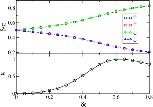
Figure 18: Phase shifts (top) and corresponding conductance (bottom) as a function of orbital splitting $\delta\epsilon$ at temperature $T=0$ (from Ref. HofstetterZarand, ).

Also, the picture outlined above changes substantially if both states $|\pm\rangle$ happen to have the same parity, and couple only to one of the fields $\psi_{+}$. In this case the conductance is small on the singlet side of the transition and exhibits a dip as a function of temperature/magnetic field.VBH However, the spin of the dot cannot be screened on the triplet side even at $T=0$ temperature, and a real Kosterlitz-Thouless type quantum phase transition occurs, where the $T=0$ temperature conductance has a jump at the transition point.VBH The triplet phase in this case is also anomalous,VBH and in fact is of a ’marginal Fermi liquid type’,marginal ; PiersPRL since the spin is not fully screened.VBH ; underscreened Correspondingly, the conductance saturates very slowly, and behaves asymptotically as $G\sim cst-1/\ln^{2}(T_{+}/T)$. Similar behavior is expected to occur if the smaller Kondo temperature $T_{-}$ is much below the measurement temperature, and indeed a behavior in agreement with the Kosterlitz-Thouless scenario of Ref. VBH, has been observed in some experiments.KoganST

V Charge fluctuations and two-channel Kondo effect at the degeneracy point

In the previous section we focussed our attention to the regimes where charge fluctuations of the dot were negligible. In the vicinity of the degeneracy points, $N_{g}\approx\mbox{half-integer}$, however, this assumption is not valid, and charge fluctuations must be treated non-perturbatively.

To have an insight how change fluctuations can lead to non-perturbative behavior, let us study the simplest circuit one can envision, the so-called single electron box (SEB), where only one lead is attached to a quantum dot (see Fig. 19). Let us furthermore focus to the limit of small tunneling and $E_{C}\gg T\gg\Delta$. The charging energy of the dot in this case is given again by Eq. (2), and the tunnel coupling to the electrode reads

$$\hat{V}=\sum_{j}\sum_{\epsilon}\Bigl{\{}t_{j}\;d^{\dagger}_{j\sigma}\psi_{\epsilon\sigma}+{\rm h.c.}\Bigr{\}}\;.$$ (30)

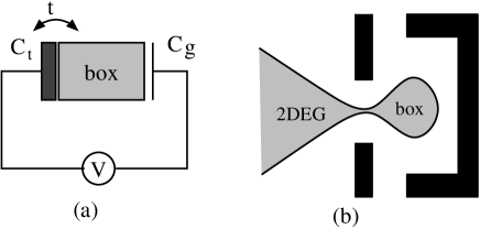
Figure 19: Sketch of the single electron box. Fig. b. shows the top view of the regime where electrons move in the the two-dimensional electron gas. Black areas indicate various electrodes necessary to shape the electron gas.

Let us now focus our attention to the regime $N_{g}\approx 1/2$, where with a good accuracy the charge on the dot fluctuates between $n_{\rm dot}=0$ and $1$. In this regime tunneling processes generated by Eq. (30) become correlated, because of the constraint that the charge of the dot must be either $0$ or $1$. To keep track of this constraint, we can introduce the pseudospin operators, $T^{+}\equiv|1\rangle\langle 0|$, $T^{-}\equiv|0\rangle\langle 1|$, and $T^{z}\equiv(|1\rangle\langle 1|-|0\rangle\langle 0|)/2$, and rewrite the tunneling part of the Hamiltonian and $H_{\rm dot}$ as

$$\hat{V} = \sum_{j}\sum_{\epsilon}\Bigl{\{}T^{+}t_{j}\;d^{\dagger}_{j\sigma}\psi_{\epsilon\sigma}+{\rm h.c.}\Bigr{\}}\;,$$ (31)

$$H_{\rm dot} = -\Delta E\;T^{z}\;$$ (32)

where $\Delta E\sim(N_{g}-1/2)$ is simply the energy difference between the two charging states of the dot. We can now attempt to compute the expectation value of the dot charge, $\langle n_{\rm dot}\rangle$ in the regime $-1/2<N_{g}<1/2$ by doing perturbation theory in $\hat{V}$ to obtain in the limit of vanishing level spacing,

$$\langle n_{\rm dot}\rangle={g\over 4\pi^{4}}\ln\Bigl{(}{1+2N_{g}\over 1-2N_{g}}\Bigr{)}+{\cal O}(g^{2})\;,$$ (33)

with $g=G/G_{Q}$ the dimensionless conductance of the junction. Although a finite level spacing cuts off the logarithmic singularity at $N_{g}=\pm 1/2$, Eq. (33) clearly indicates that perturbation theory breaks down in the vicinity of the degeneracy points.

In fact, following the mapping originally proposed by Matveev,Matveev we shall now show that the Hamiltonian above can be mapped to that of the two-channel Kondo problem. To perform the mapping, we rewrite the tunneling Hamiltonian in a more suggestive way by introducing the new fields normalized by the density of states in the box and in the lead, $\varrho_{\rm dot}$ and $\varrho_{\rm lead}$, respectively

$$D_{\sigma}\equiv{1\over\sqrt{\varrho_{\rm box}}}\sum_{j}d_{j,\sigma}\;,\phantom{nn}C_{\sigma}\equiv{1\over\sqrt{\varrho_{\rm lead}}}\sum_{\epsilon}\psi_{\epsilon,\sigma}\;,$$ (34)

and organize them into a four component spinor

$$\psi_{\tau,\sigma}\equiv\pmatrix{C_{\sigma}\cr D_{\sigma}\cr}\;.$$ (35)

In the limit $\Delta\to 0$ the tunneling amplitudes can be simply replaced by their average, $t_{j}\to t\equiv\langle|t_{j}|^{2}\rangle_{j}^{1/2}$, and we can rewrite the tunneling part of Hamiltonian as

$$H_{\rm perp}={j_{\perp}\over 2}\sum_{\sigma}(T^{+}\psi^{\dagger}_{\sigma}\tau^{-}\psi_{\sigma}+{\rm h.c.})\;,$$ (36)

where the operator $\tau^{\pm}$ just flips the orbital spin $\tau$ of the field $\psi_{\tau\sigma}$, and $j_{\perp}$ is a dimensionless coupling proportional to the tunneling, $j_{\perp}=2t\sqrt{\varrho_{\rm box}\varrho_{\rm lead}}$. Thus $j_{\perp}^{2}\sim t^{2}{\varrho_{\rm box}\varrho_{\rm lead}}$ is directly related to the dimensionless conductance $g$ of the tunnel junction

$$g={\pi^{2}}j_{\perp}^{2}\;.$$ (37)

Eq. (36) is just the Hamiltonian of an anisotropic two-channel Kondo model,Matveev ; Cox the orbital spins $T$ and $\tau$ playing the role of the spins of the original two-channel Kondo model, and the electron spin $\sigma$ providing a silent channel index. The presence of this additional channel index (electron spin) makes the physics of the two-channel Kondo model entirely different from that of the single channel Kondo problem, and leads to non-Fermi liquid properties:Cox The low temperature conductance between the dot and the lead turns out to scale to $g(T\to 0)\to e^{2}/h$ with a $\sqrt{T}$ singularity and the capacitance diverges logarithmically as $N_{g}\to 1/2$ and $T\to 0$.Matveev Thus the theory of Matveev predicts that the sharp steps in $\langle n_{\rm dot}\rangle$ become smeared out as shown in Fig. 3, although the slope of the steps diverges at the degeneracy points.

This is, however, not the full picture. Very recently, Karyn le Hur studied the effect of dissipative coupling to other leads in the circuit, and showed that if these additional leads are resistive enough, then the dissipation induced by them leads to a phase transition, where the steps are restored.LeHur This transition can be shown by bosonization methods to be of Kosterlitz-Thouless type.NoisyBox In Fig. 20 we show the shape of the step computed using numerical renormalization group methods for the single channel case (spinless fermions) that clearly shows the above phase transition.NoisyBox

Figure 20: The expectation value of $n_{\rm dot}-1/2$ for different values of $\alpha$. For moderate values of the bosonic coupling the step is smeared out by quantum fluctuations of the charge of the dot. The step gets sharper and sharper as $\alpha$ approaches $\alpha_{c}$, and For $\alpha>\alpha_{c}$ a jump appears in $\langle{\hat{n}}_{\rm dot}\rangle$ (from Ref. NoisyBox, ).

We emphasize again, that the above mapping holds only in the regime $\Delta<T,\omega,...<E_{C}$, where the level spacing of the box can be neglected, and is only valid for the case of a single mode contact, Unfortunately, for small semiconductor dots with large enough $E_{C}$ the ratio $E_{C}/\Delta$ is not very large,Berman ; Wilhelm and therefore the regime where the two-channel Kondo behavior could be observed is rather limited. In fact, this intriguing two-channel Kondo behavior has never been observed convincingly experimentally.Berman

The ratio $E_{C}/\Delta$ can be much larger in metallic grains,Devoret ; Schoen However, metallic grains have been connected so far only through leads with a large number of conduction modes, and the behavior of these systems is rather different from what we discussed so far: They can be described by an infinite channel Kondo model,Schoen which predicts, e.g., that the junction conductance goes to zero logarithmically at the degeneracy point in the $T\to 0$ limit, $g_{\rm metal}(T)\sim 1/\ln^{2}(T/T_{K})$, in clear disagreement with the two-channel Kondo predictions. It turns out, that for a finite number $N_{c}$ of conductance modes a new temperature scale $T^{*}$ appears:Wilhelm Above this scale the conductance decreases as $\sim 1/\ln^{2}(T)$, while below this scale it increases and approaches the two-channel Kondo value $g=e^{2}/h$. Unfortunately, this scale goes to zero exponentially fast with the number of modes, $T^{*}\sim\exp(-C\;N_{c})$. Therefore, one really needs to prepare single mode contacts to observe the two-channel Kondo behavior in metallic grains, which is a major experimental challenge.

Recently, another realization of the two-channel Kondo behavior has also been proposed in semiconductor devices, where one has a somewhat better control of the Kondo scale and $E_{C}/\Delta$ than in single electron boxes.Oreg ; Eran

So far we discussed only the limit of small level spacing $\Delta\to 0$. The physics of the degeneracy point $N_{g}=1/2$ remains also rather non-trivial in the limit $T\ll\Delta$. In this regime the dot behaves as a mixed valence atom, and charge fluctuations are huge.Hewson The description of these mixed valence fluctuations is a rather complicated problem, and requires non-perturbative methods such as the application of numerical renormalization group.Theo

VI Conclusions

In the present paper we reviewed some of the interesting strongly correlated states that can be realized using quantum dots. These artificial structures behave in many respects like artificial atoms, excepting the difference in the energy scales that characterize them. Having a full control over these devices opened up the possibility of building structures that realize unusual strongly correlated states like the ones discussed in this paper, that are very difficult to observe in atomic physics. This technology also enabled one to study out of equilibrium and transport properties of such individual ’atoms’.

However, building quantum dots and quantum wires is just the first step towards a new technology, which aims to construct devices from real atoms and molecules instead of mesoscopic structures. Although a real breakthrough took place in recent years, and molecules have been contacted and used to construct single electron transistors,molecular_SET the technology is far from being controlled.

Building (gated) quantum dot arrays in a controlled way has not been solved satisfactorily yet either. Having a handle on such systems could give way to study quantum phase transitions in lattices of artificial atoms in the laboratory. Experimentalists are also facing the challenge of producing hybrid structures at the nanoscale: these structures can hopefully be used in future spintronics applications or quantum computing.

There is a lot of open questions on the theoretical side as well: As we mentioned already, the problem of treating strongly correlated systems in out of equilibrium is unsolved even for simple toy models, and it is still a dream to study molecular transport through correlated out of equilibrium atomic clusters by combining ab initio and many-body methods. Moreover, many important questions like the interplay of ferromagnetism and strong correlations in ferromagnetic grains have not been studied in sufficient detail.

I would like to thank all my collaborators, especially Laszló Borda, Walter Hofstetter, and A. Zawadowski for the valuable discussions. This research has been supported by Hungarian Grants No. OTKA T038162, T046267, and T046303, and the European ’Spintronics’ RTN HPRN-CT-2002-00302.

Appendix A Hartree approximation for a quantum dot

To derive Eq. (2), let us consider a metallic grain within the Hartree approximation. Then the wave functions $\varphi_{j}$ must be determined self-consistently by solving the following equations:

$$\Bigl{(}-{\Delta\over 2m}+V_{H}(\vec{r})\Bigr{)}\varphi_{j}=E_{j}\;\varphi_{j}\;,$$

$$V_{H}(\vec{r})=V(\vec{r})+\int d{\vec{r}}^{\prime}U({\vec{r}}-{\vec{r}}^{\prime})\varrho({\vec{r}}^{\prime})\;,$$ (38)

where $V$ is the confining potential generated by the positively charged ions, $U$ is the electron-electron interaction, and $V_{H}$ is the Hartree potential. The electronic density $\varrho({\vec{r}})$ in Eq. (38) must be computed as $\varrho({\vec{r}})=\sum_{j,\sigma}n_{j,\sigma}\;|\varphi_{j}|^{2}$, with $n_{j,\sigma}$ the occupation number of the levels.

The total energy of the system with $N=\sum_{j,\sigma}n_{j,\sigma}$ electrons is

$$E^{N}_{H}=\sum_{j,\sigma}E_{j}\;n_{j,\sigma}-{1\over 2}\int d{\vec{r}}\;d{\vec{r}}^{\prime}\varrho({\vec{r}})V({\vec{r}}-{\vec{r}}^{\prime})\varrho({\vec{r}}^{\prime})\;,$$ (39)

where the second term compensates for overcounting the electron-electron interaction. In order to compute the energy cost of adding another electron to the grain, we should solve selfconsistently Eqs. (38) for $\sum_{j,\sigma}n_{j,\sigma}=N+1$, compute $E^{N+1}_{H}$ and then determine the difference between these two energies, $E^{N+1}_{H}-E^{N}_{H}$. However, one can approximately compute this energy by just noticing that the charge of the extra electron in state $N+1$ must go to the surface of the grain to produce an approximately constant potential inside the grain, and is screened within a layer of the Fermi wavelength $\sim\lambda_{F}$. The change in the Hartree potential is simply given as

$$\delta V_{H}=\int d{\vec{r}}^{\prime}U({\vec{r}}-{\vec{r}}^{\prime})\;\delta\varrho({\vec{r}}^{\prime})\;.$$ (40)

But since the change of the electronic density can be very well approximated by a classical surface charge for a grain size $L\gg\lambda_{F}$, $\delta V_{H}$ is just the classical potential of the charged grain. Consequently, $\delta V_{H}\approx e^{2}/C$ inside the metallic grain. Using this simple fact we find that adding an extra electron to the grain shifts all Hartree energies as $E_{j}\to E_{j}+e^{2}/C$ and requires an energy

$$E^{+}\approx E_{f}+{e^{2}\over 2C}\;,$$ (41)

with $E_{f}$ the Hartree energy of the first unoccupied level, and $C$ the classical capacitance of the grain. Defining the chemical potential as the Hartree energy of the last occupied level, $\mu\equiv\epsilon_{l}$ and defining the quasiparticle energies as $\epsilon_{j}\equiv E_{j}-\mu$ we find by extending the above analysis to the excited states as well that the energy of the dot is approximately described by Eqs. (1) and (2). Note that for an isolated dot this analysis gives $N_{g}=-\mu C/e^{2}$, which is usually not equal to zero, so adding and removing an electron requires different energies, just as in case of an atom.

References

- (1) D. Goldhaber-Gordon, H. Shtrikman, D. Mahalu, D. Abusch-Magder, U. Meirav, and M.A. Kastner, Nature (London) 391, 156 (1998)
- (2) S. Tarucha D.G. Austing, Y. Tokura, W.G. van der Wiel, and L.P. Kouwenhoven, Phys. Rev. Lett. 84, 2485 (2000);
- (3) L.P. Kouwenhoven, D.G. Austing, S. Tarucha, Rep. Prog. Phys. 64, 701 (2001).
- (4) P. Joyez et al., Phys. Rev. Lett. 79, 1349 (1997).
- (5) Ralph DC, Black CT, Tinkham M Phys. Rev. Lett. 78, 4087 (1997).
- (6) J. Park et al., Nature (London) 417, 722 (2002); W. J. Liang et al., Nature (London) 417, 725 (2002).
- (7) R. Wilkins, E. Ben-Jacob, and R. C. Jaklevic, Phys. Rev. Lett. 63, 801 (1989).
- (8) S.M. Cronenwett, T.H. Oosterkamp, and L.P. Kouwenhoven, Science 281, 540 (1998).
- (9) L. I. Glazman and M. E. Raikh, JETP Lett. 47, 452 (1988); T. K. Ng and P. A. Lee, Phys. Rev. Lett. 61, 1768 (1988).
- (10) N. Andrei, G.T. Zimanyi and G. Schön, Phys. Rev. B 60, 5125 (R) (1999).
- (11) G. Zaránd, G.T. Zimányi, and F. Wilhelm, Phys. Rev. B 62, 8137 (2000).
- (12) I.L. Aleiner, P.W. Brouwer, and L.I. Glazman, Physics Reports 358, 309 (2002).
- (13) M. L. Mehta, Random Matrices (Academic Press, New York, 1991).
- (14) D. S. Golubev, J. K nig, H. Schoeller, G. Sch n, and A. D. Zaikin, Phys. Rev. B 56, 15782 (1997); J. K nig and H. Schoeller, Phys. Rev. Lett. 81, 3511 (1998);
- (15) I.O. Kulik and R.I. Shekhter, Zh. Eksp. Teor. Fiz. 62 (1975) 623 [Sov. Phys. JETP 41 (1975) 308]; L.I. Glazman and R.I. Shekhter, Journ. of Phys.: Condens. Matter 1 (1989) 5811.
- (16) D.V. Averin and Yu.V. Nazarov, Phys. Rev. Lett. 65 (1990) 2446.
- (17) A.C. Hewson, The Kondo Problem to Heavy Fermions (Cambridge Un iversity Press, Cambridge, 1993).
- (18) P.W. Anderson, Journ. of Physics C3 (1970) 2436; Abrikosov A.A. and Migdal A.A., J. Low Temp. Phys. 3 519 (1970); Fowler M. and Zawadowski A., Solid State Commun. 9, 471 (1971).
- (19) The Friedel sum rule can be only applied in our case at temperature, where the impurity spin is screened and disappears from the problem, and conduction electrons at the Fermi surface experience only some residual scattering. The Friedel sum rule has rigorously been derived only for the Anderson Hamiltonian, where it relates the number of electrons on the dot to the phase shifts. [See D.C. Langreth, Phys. Rev. 150, 516 (1966)]. In case of the Kondo problem, there seems to be an ambiguity modulo in the phase shift’s definition.
- (20) T. A. Costi Phys. Rev. B 64, 241310 (2001); T. Costi, Phys. Rev. Lett. 85, 1504 (2000).
- (21) Y. Meir, N. S. Wingreen, and P. A. Lee, Phys. Rev. Lett. 70, 2601-2604 (1993).
- (22) A. Rosch, J. Paaske, J. Kroha, and P. W lfle, Phys. Rev. Lett. 90, 076804 (2003).
- (23) P. Coleman, C. Hooley, and O. Parcollet, Phys. Rev. Lett. 86, 4088-4091 (2001).
- (24) A. Schiller and S. Hershfield, Phys. Rev. B 58, 14978-15010 (1998); A. Schiller and S. Hershfield, Phys. Rev. B 51, 12896-12899 (1995).
- (25) G. Zaránd, A. Brataas, and D. Goldhaber-Gordon, Solid State Commun. 126, 463-466 (2003).
- (26) W.G. van der Wiel et al., Phys. Rev. Lett. 88, 126803 (2002).
- (27) L. Borda, G. Zaránd, W. Hofstetter, B. I. Halperin, and Jan von Delft, Phys. Rev. Lett. 90, 026602 (2003).
- (28) S. Sasaki et al., Nature 405, 764 (2000).
- (29) A. Kogan et al., Phys. Rev. B 67, 113309 (2003).
- (30) Wilhelm U, Weis J Physica E 6, 668 (2000).
- (31) S. Sasaki, S. Amaha, N. Asakawa, M. Eto and S. Tarucha, Phys. Rev. Lett. 93, 17205 (2004).
- (32) P. Jarillo-Herrero et al., to appear in Nature.
- (33) K. Le Hur and P. Simon, Phys. Rev. B 67, 201308 (2003).
- (34) K. Le Hur, P. Simon, and L. Borda, Phys. Rev. B 69, 045326 (2004)
- (35) L. D. Leo and M. Fabrizio, Phys. Rev. B 69, 245114 (2004).
- (36) K.G. Wilson, Rev. Mod. Phys. 47, 773 (1975).
- (37) G. Zaránd, Phys. Rev. Lett. 77, 3609 (1996).
- (38) A. Tsvelik and P. Wiegman, Adv. Phys. 32, 453 (1983).
- (39) B. Coqblin and J. R. Schrieffer, Phys. Rev. 185, 847 (1969).
- (40) P. Nozieres and A. Blandin, J. Physique 41, 193 (1980).
- (41) A Zeeman field corresponds to a field applied parallel to the surface in a lateral quantum dot experiment.
- (42) R. Landauer, IBM J. Res. Dev. 1, 223 (1957); D.S. Fisher and P.A. Lee, Phys. Rev. B 23, 6851 (1981); M. Büttiker, Phys. Rev. Lett. 57, 1761 (1986).
- (43) M. Pustilnik and L. I. Glazman, Phys. Rev. Lett. 85, 2993 (2000); Phys. Rev. B 64, 045328 (2001).
- (44) W. Hofstetter and G. Zarand, Phys. Rev. B 69, 235301 (2004).
- (45) T. Jamnaela et al., Phys. Rev. Lett. 87, 256804 (2001).
- (46) B. Lazarovits et al, cond-mat/0407399.
- (47) B. C. Paul and K. Ingersent, cond-mat/9607190.
- (48) M. Eto and Yu.V. Nazarov, Phys. Rev. Lett. 85, 1306 (2000); Phys. Rev. B 66, 153319 (2002).
- (49) M. Pustilnik and L.I. Glazman, Phys. Rev. Lett. 87, 216601 (2001); M. Pustilnik, L. I. Glazman and W. Hofstetter: Phys. Rev. B 68 (2003) 161303(R).
- (50) W. Hofstetter, H. Schoeller, Phys. Rev. Lett. 88, 016803 (2002); M. Vojta, R. Bulla, and W. Hofstetter, Phys. Rev. B 65, 140405 (2002).
- (51) P. Mehta, L. Borda, G. Zaránd, N. Andrei, P. Coleman, cond-mat/0404122.
- (52) A. Posazhennikova and P. Coleman, cond-mat/0410001 (accepted for publication in Phys. Rev. Lett.).
- (53) For the thermodynamical properties of the underscreened Kondo problem, see N. Andrei, K. Furuya, and J. H. Lowenstein, Rev. Mod. Phys., 51, 331 (1983).
- (54) bi K.A. Matveev, Zh. Eksp. Teor. Fiz. 98, 1598 (1990) [Sov. Phys. JETP 72, 892 (1991)]; Phys. Rev. B 51, 1743 (1995).
- (55) For a review on the two-channel Kondo problem see D.L. Cox and A. Zawadowski, Adv. Phys. 47, 599 (1998).
- (56) K. Le Hur, Phys. Rev. Lett. 92, 196804 (2004)
- (57) L. Borda, G. Zaránd, and P. Simon, cond-mat/0412330.
- (58) D. Berman, N.B. Zhetinev, and R.C. Ashoori, Phys. Rev. Lett. 82, 161 (1999).
- (59) Y. Oreg and D. Goldhaber-Gordon, Phys. Rev. Lett. 90, 136602 (2003).
- (60) F. B. Anders, E. Lebanon, and A. Schiller, Phys. Rev. B 70, 201306 (2004).