Thermal Brownian motor

Abstract

Recently, a thermal Brownian motor was introduced [Van den Broeck, Kawai and Meurs, Phys. Rev. Lett., 2004], for which an exact microscopic analysis is possible. The purpose of this paper is to review some further properties of this construction, and to discuss in particular specific issues including the relation with macroscopic response and the efficiency at maximum power.

1 Introduction

Brownian motors are small scale engines that operate on the basis of nonequilibrium fluctuations. Most of the models that have been discussed previously in the literature refer to the transfer of chemical or potential energy into work [1] by Brownian entities that operate in a externally imposed asymmetric environment (or by spontaneous symmetry breaking [2]). In this case, a $100$ percent efficiency can in principle be achieved [3], in accordance with the basic laws of thermodynamics. Recently, a thermal Brownian motor was introduced [4], for which an exact microscopic analysis turns out to be possible [5]. The model can be viewed as a simplification of the Feynman-Smoluchowski ratchet [6, 7]. This construction differs in two essential aspects from most other Brownian motors. First, the source of energy is the presence of different heat baths. Thermodynamics thus predicts that the limiting efficiency is that of the Carnot engine. Second, the asymmetry is an intrinsic property of the motor, not of the environment or of the imposed constraint. The purpose of this paper is to review some further properties of this construction, and to discuss in particular specific issues including the relation with macroscopic response and the efficiency at maximum power.

2 Model and basic results

We first briefly review the basic construction of the thermal Brownian motor and the main results. The motor consists of a set of convex units $i$ ($i=1,...,N$), that move as a rigidly linked entity with a single degree of freedom, along a specified direction $x$. Each unit resides in a separate, infinitely large compartment that is filled with an ideal gas at equilibrium. These compartments play a role akin to the thermal reservoirs in a Carnot construction. For simplicity, we consider the case of spatial dimension $d=2$ with coordinates $(x,y)$. In Fig. 1 we show four different realizations of the motor. The gas particles are point particles of mass $m$. Their density, temperature and Maxwellian velocity distribution in compartment $i$ are denoted by $\rho_{i}$, $T_{i}$ and $\phi_{i}$ respectively, with:

$$\phi_{i}(v_{x},v_{y})=\frac{m}{2\pi k_{B}T_{i}}\exp{\left(\frac{-m(v_{x}^{2}+v_{y}^{2})}{2k_{B}T_{i}}\right)}.$$ (1)

We consider the limit in which the mean free path of the gas particles is much larger than the linear dimension of the motor unit. In this case, there are no pre-collisional correlations between the speed of the motor and that of the impinging particles. The probability density $P(V,t)$ for the speed $\vec{V}=(V,0)$ therefore obeys a Boltzmann-Master equation:

$$\frac{\partial P(V,t)}{\partial t}=\int{dV^{\prime}\Big{[}W(V|V^{\prime})P(V^{\prime},t)-W(V^{\prime}|V)P(V,t)\Big{]}.}$$ (2)

$W(V|V^{\prime})=\sum_{i}W_{i}(V|V^{\prime})$ is the transition probability per unit time for the motor to change speed from $V^{\prime}$ to $V$ due to the collisions with the gas particles in the compartments $i=1,\ldots,N$. Its explicit form, following from the collision rules and basic arguments from kinetic theory, is given by (see [5] for more details):

$$W_{i}(V|V^{\prime})=\int_{0}^{2\pi}d\theta\,S_{i}F_{i}(\theta)\int_{-\infty}^{+\infty}dv_{x}^{\prime}\int_{-\infty}^{+\infty}dv_{y}^{\prime}\rho_{i}\phi_{i}(v_{x}^{\prime},v_{y}^{\prime})(\vec{V}^{\prime}-\vec{v}^{\prime})\cdot\hat{e}_{\perp}$$

$$\times\Theta\left[(\vec{V}^{\prime}-\vec{v}^{\prime})\cdot\hat{e}_{\perp}\right]\delta\left[V-V^{\prime}-\frac{2\frac{m}{M}\sin^{2}\theta}{1+\frac{m}{M}\sin^{2}\theta}\left(v_{x}^{\prime}-v_{y}^{\prime}\cot\theta-V^{\prime}\right)\right].$$ (3)

Here $\Theta$ is the Heaviside step function. The $\delta$ Dirac function selects appropriate particle velocities yielding the post-collisional speed $V$ for the motor in function of the precollisional speeds $V^{\prime}$ and $v^{\prime}_{x},v^{\prime}_{y}$ of motor and gas particle respectively. The shape of the motor unit $i$ is characterized by a normalized shape function $F_{i}(\theta)$, such that $F_{i}(\theta)d\theta$ is the fraction of the outer surface of the unit that has a tangent between $\theta$ and $\theta+d\theta$, cf. Fig. 2. The angle $\theta$ is measured counterclockwise from the horizontal $x$ direction. The total perimeter will be denoted by $S_{i}$.

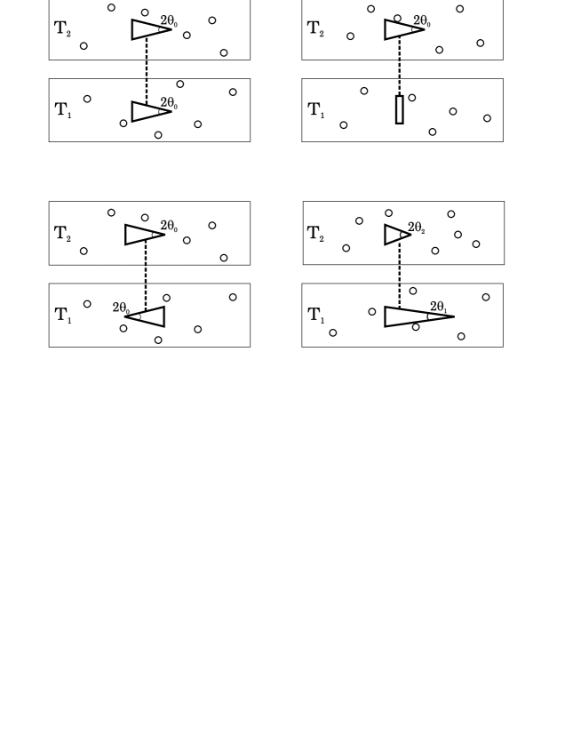
Figure 1: Four different realizations of the thermal Brownian motor, each consisting of two rigidly linked motor units. (a) will be referred to as Triangula and is composed out of two identical triangles, while model (b) is called Triangulita and has a triangle and a bar. Constructions (c) and (d) consist respectively out of two identical triangles pointing in the opposite direction and two triangles with a different apex angle.

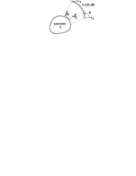
Figure 2: A closed and convex object with perimeter $S$. The length of the surface with an orientation between $\theta$ and $\theta+d\theta$ is $SF(\theta)d\theta$, defining the form factor $F(\theta)$.

Solving the Boltzmann-Master equation in general is out of the question, even at the steady state. To make progress, a perturbative solution is necessary. Since we expect that the rectification disappears in the limit of a macroscopic motor, a natural expansion parameter is the ratio of the mass $m$ of the gas particle over the mass $M$ of the object. More precisely, we have used $\varepsilon=\sqrt{m/M}$ as the expansion parameter.

Introducing the transition probability $W_{i}(V^{\prime};r)=W_{i}(V|V^{\prime})$ with jump amplitude $r=V-V^{\prime}$, the Boltzmann equation can be rewritten as

$$\frac{\partial P(V,t)}{\partial t} = \int{W(V-r;r)P(V-r,t)dr}-P(V,t)\int{W(V;-r)dr}.$$ (4)

The Taylor expansion of the r.h.s. of this equation with respect to the jump amplitude leads to the equivalent Kramers-Moyal expansion:

$$\frac{\partial P(V,t)}{\partial t}=\sum_{n=1}^{\infty}{\frac{(-1)^{n}}{n!}\left(\frac{d}{dV}\right)^{n}\left\{a_{n}(V)P(V,t)\right\},}$$ (5)

with jump moments $a_{n}(V)=\sum_{i}a_{n,i}(V)$, defined as:

$$a_{n,i}(V)=\int{r^{n}W_{i}(V;r)dr}.$$ (6)

One can obtain from the Kramers-Moyal expansion the set of coupled equations for the moments of the velocity distribution $\langle V^{n}\rangle=\int V^{n}P(V,t)$. Of interest for the subsequent discussion, we reproduce the exact results for the first two moment equations:

$$\partial_{t}\langle V\rangle = \langle a_{1}(V)\rangle$$ (7)

$$\partial_{t}\langle V^{2}\rangle = 2\langle Va_{1}(V)\rangle+\langle a_{2}(V)\rangle,$$ (8)

with

$$a_{1,i}(V)=-\rho_{i}S_{i}\int_{0}^{2\pi}d\theta F_{i}(\theta)\frac{1}{M+m\sin^{2}{\theta}}$$

$$\left[\sqrt{\frac{2k_{B}T_{i}m}{\pi}}\exp[-\frac{m}{2k_{B}T_{i}}V^{2}\sin^{2}{\theta}]V\sin^{2}{\theta}+\right.$$

$$+\left.\left(1+\textrm{Erf}\left[\sqrt{\frac{m}{2k_{B}T_{i}}}V\sin{\theta}\right]\right)\left(k_{B}T_{i}\sin{\theta}+mV^{2}\sin^{3}{\theta}\right)\right]$$ (9)

$$a_{2,i}(V)=2\rho_{i}S_{i}\int_{0}^{2\pi}d\theta F_{i}(\theta)\frac{\sin^{2}\theta}{(M+m\sin^{2}{\theta})^{2}}$$

$$\left[\sqrt{\frac{2k_{B}T_{i}m}{\pi}}\exp[-\frac{m}{2k_{B}T_{i}}V^{2}\sin^{2}{\theta}]\left(2k_{B}T_{i}+mV^{2}\sin^{2}{\theta}\right)+\right.$$

$$+\left.\left(1+\textrm{Erf}\left[\sqrt{\frac{m}{2k_{B}T_{i}}}V\sin{\theta}\right]\right)\left(3k_{B}T_{i}mV\sin{\theta}+m^{2}V^{3}\sin^{3}{\theta}\right)\right].$$ (10)

3 Systematic speed: general results

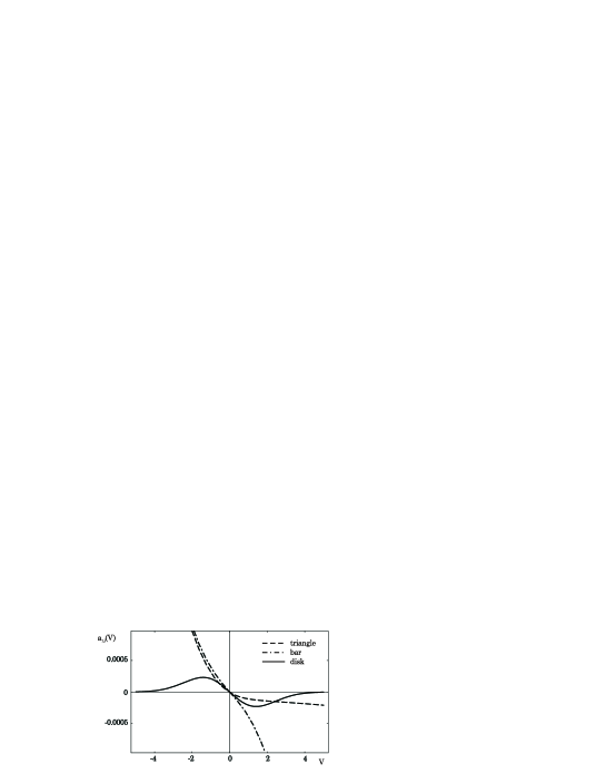
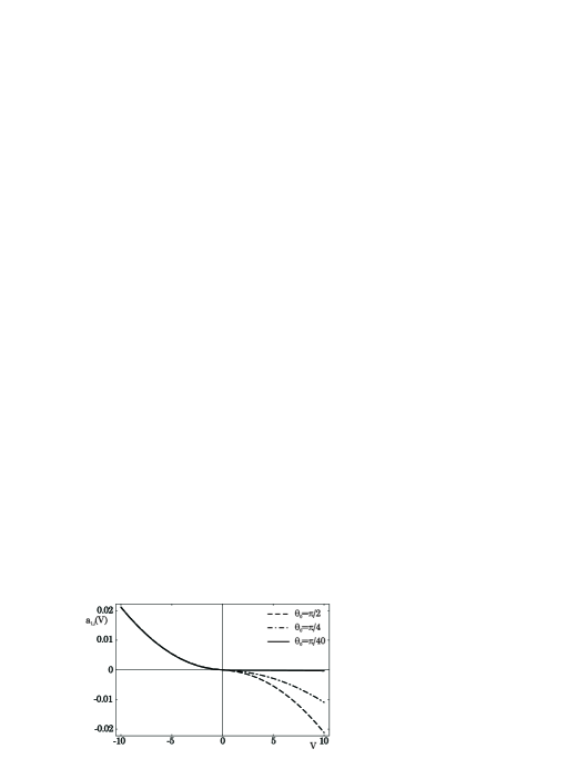
Figure 3: (a) Top: The response function $a_{1,i}(V)$, see Eq. (9), for different geometric objects used in de constructions of Fig. 1: a triangle with $\theta_{0}=\pi/36$, a bar of length $L$ and a disk with radius $R$.
(b) Bottom: The function $a_{1,i}(V)$ for a triangle with opening angle respectively equal to $\pi,\pi/2$ and $\pi/20$. The following parameter values were used: mass ratio $M/m=20$, density $\rho_{i}=0.0022$, temperature $T_{i}=1$, size $L=R=1$ and $k_{B}=1$ by choice of units.

The equation for the first moment is coupled to the higher moments, a familiar feature in statistical mechanics. However, a perturbative solution can be obtained by considering the Taylor expansion in $\varepsilon$. To lowest order in $\varepsilon$ the first moment equation reduces to a closed equation featuring a linear relaxation law, namely:

$$M\partial_{t}\langle V\rangle=-\gamma\langle V\rangle,$$ (11)

where $\gamma=\sum_{i}\gamma_{i}$ and $\gamma_{i}$ the linear friction coefficient, due to the section of the motor sitting in gas mixture $i$:

$$\gamma_{i}=4\rho_{i}S_{i}\sqrt{\frac{k_{B}T_{i}m}{2\pi}}\int_{0}^{2\pi}{d\theta F_{i}(\theta)\sin^{2}{\theta}}.$$ (12)

Note that at this level of the perturbation, the steady state speed of the motor is zero: even though the motor may be constituted of asymmetric parts, no rectification takes place at the level of linear response.

At the next order in the perturbation, the first moment is coupled to the second one, which needs to be solved at lowest order. By doing so, one finds at the steady state:

$$M\langle V^{2}\rangle=k_{B}T_{\mathrm{eff}},$$ (13)

with $T_{\mathrm{eff}}$ the effective temperature given by:

$$T_{\mathrm{eff}}=\frac{\sum_{i}{\gamma_{i}T_{i}}}{\sum_{i}{\gamma_{i}}}.$$ (14)

By inserting this result in the equation for the average velocity, one finds for the lowest order term of the steady state velocity $V_{0}$:

$$V_{0}\equiv\langle V\rangle=\sqrt{\frac{m}{M}}\sqrt{\frac{\pi k_{B}T_{\mathrm{eff}}}{8M}}\frac{\sum_{i}\rho_{i}S_{i}\left(\frac{T_{i}}{T_{\mathrm{eff}}}-1\right)\int_{0}^{2\pi}d\theta F_{i}(\theta)\sin^{3}\theta}{\sum_{i}\rho_{i}S_{i}\sqrt{\frac{T_{i}}{T_{\mathrm{eff}}}}\int_{0}^{2\pi}d\theta F_{i}(\theta)\sin^{2}(\theta)}.$$ (15)

This speed is equal to the expansion parameter times the thermal speed of the motor and further multiplied by a factor that depends on the geometric properties of the object. Note that the Brownian motor ceases to function in the absence of a temperature difference (when $T_{i}=T_{\mathrm{eff}}$ for all $i$) and in the macroscopic limit $M\rightarrow\infty$ (since $V_{0}\sim 1/M$). Note also that the speed is scale-independent, i.e., independent of the actual size of the motor units: $V_{0}$ is invariant under the rescaling $S_{i}$ to $CS_{i}$. In Table 1 we have collected the explicit result for $V_{0}$ for the four different thermal motors, depicted in Fig. 1.

It is tempting to interpret the direction of the systematic speed on the basis of intuition. One can study the response of the motor by the application of an external force. Due to the asymmetry, the response curve (speed versus force) will be asymmetric. In particular, it will require less force to move a triangle in the “easy” direction of the sharp angle. Consequently, one expects that fluctuations leading to an “extra force” in the easy direction would be more successful in moving the object than the ones in the other direction. A similar argument can be applied to the discussion of the electric current in a diode, which also has an asymmetric response of current versus field. One expects that fluctuations in the electric field will produce a larger current in one direction than in the other one. However, as is well known [8], these arguments are clearly wrong. The first observation is that there is no systematic speed (or electric current) when the system is at equilibrium. In fact, the effect of possible asymmetries in a system are completely wiped out in equilibrium, as expressed explicitly in the principle of detailed balance discovered by Onsager [9]: at equilibrium any process and its time-reverse occur equally frequently. Second, equilibrium is typically a so-called point of flux reversal [7]. For example, in the case of Triangulita, the flux is in the “easy” direction of the sharp angle, only in the case when the temperature is lower in the reservoir containing the triangle. Otherwise the speed is in the opposite direction. Furthermore the speed again becomes zero when the temperature is zero in the reservoir containing the flat paddle. Finally, the above mentioned asymmetry in the response appears in the nonlinear regime. In this regime, the dynamics of the various moments are however coupled. In particular, the equation for the average speed is not closed, but depends on the entire probability distribution. The nonlinear response to an external force is therefore not linked in an obvious way to the intrinsic nonlinear dynamics generated by nonequilibrium fluctuations.

Full information on the equation of the first moment is contained in the nonlinear function $a_{1,i}(V)$. It is reproduced in figures 3(a) and 3(b) for the motor units used in the constructions of Fig. 1. However, the direction of motion, to lowest order in $\varepsilon$, contains much less information. Indeed, from Eq. (15), one finds for a motor with $2$ units:

$$\mathrm{sgn}(V_{0})=\mathrm{sgn}\left[(T_{1}-T_{2})\left(\frac{\langle\sin^{3}{\theta}\rangle_{{}_{1}}}{\langle\sin^{2}{\theta}\rangle_{{}_{1}}}-\sqrt{\frac{T_{1}}{T_{2}}}\frac{\langle\sin^{3}{\theta}\rangle_{{}_{2}}}{\langle\sin^{2}{\theta}\rangle_{{}_{2}}}\right)\right].$$ (16)

Hence the direction of the average speed does not depend on the densities of the gases or the size of the motor units. The quantity $-1\leq\langle\sin^{3}\theta\rangle_{{}_{i}}=\int_{0}^{2\pi}d\theta F_{i}(\theta)\sin^{3}\theta\leq 1$ is a measure for the sharpness of the unit:

$$\langle\sin^{3}\theta\rangle\ \ \ \left\{\begin{array}[]{ll}\rightarrow 1&\textrm{infinitely sharp to the left}\\ =0&\textrm{symmetric upon reflection about $y$-axis}\\ \rightarrow-1&\textrm{infinitely sharp to the right}.\end{array}\right.$$ (20)

On the other hand the quantity $0\leq\langle\sin^{2}{\theta}\rangle\leq 1$ is proportional to the linear friction coefficient, cf. Eq. (12). For a bar of zero width, it has the minimal value $\langle\sin^{2}{\theta}\rangle=0$ when the bar is oriented horizontally, while it is maximal ($\langle\sin^{2}{\theta}\rangle=1$) for a vertical bar.

Shape	Fig.	Stationary velocity $V_{0}$ (order $\varepsilon$)
Triangula	1(a)	$\frac{\sqrt{2\pi k_{B}m}}{4M}(1-\sin{\theta_{0}})\frac{\rho_{1}\rho_{2}(T_{1}-T_{2})(\sqrt{T_{1}}-\sqrt{T_{2}})}{\left[\rho_{1}\sqrt{T_{1}}+\rho_{2}\sqrt{T_{2}}\right]^{2}}$
Triangulita	1(b)	$\frac{\sqrt{2\pi k_{B}m}}{4M}(1-\sin^{2}{\theta_{0}})\frac{2\rho_{1}\rho_{2}\sqrt{T_{1}}(T_{1}-T_{2})}{\left[2\rho_{1}\sqrt{T_{1}}+\rho_{2}\sqrt{T_{2}}(1+\sin{\theta_{0}})\right]^{2}}$
Triangle - triangle ($\rhd\lhd$)	1(c)	$\frac{\sqrt{2\pi k_{B}m}}{4M}(1-\sin{\theta_{0}})\frac{\rho_{1}\rho_{2}(T_{1}-T_{2})(\sqrt{T_{1}}+\sqrt{T_{2}})}{\left[\rho_{1}\sqrt{T_{1}}+\rho_{2}\sqrt{T_{2}}\right]^{2}}$
Triangle - triangle ($\theta_{1}\neq\theta_{2}$)	1(d)	$\frac{\sqrt{2\pi k_{B}m}}{4M}\frac{\rho_{1}\rho_{2}(1+\sin\theta_{1})(1+\sin\theta_{2})(T_{1}-T_{2})[\sqrt{T_{1}}(1-\sin\theta_{2})-\sqrt{T_{2}}(1-\sin\theta_{1})]}{\left[\rho_{1}\sqrt{T_{1}}(1+\sin\theta_{1})+\rho_{2}\sqrt{T_{2}}(1+\sin\theta_{2})\right]^{2}}$

Table 1: Analytic result for the lowest order contribution to $\langle V\rangle$ for the different constructions depicted in Fig. 1.

Based on Eq. (16), one can distinguish four different classes of motors, depending on how the direction of speed is affected upon interchanging the temperatures $T_{1}$ and $T_{2}$. The examples of Fig. 1 each represent one such class. Fig. 4 illustrates their behavior upon switching $T_{1}$ and $T_{2}$.

4 Systematic speed: special cases

To gain further insight on the direction of the systematic speed, it is instructive to calculate its explicit value for a number of special cases, see also Table 1.

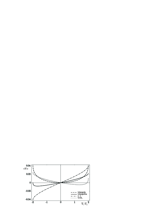
Figure 4: Plot of the average speed (see Table 1) for the four different models depicted in Fig. 1 as a function of the applied temperature difference. The following parameter values are used: $M/m=20$, $\rho_{1}=\rho_{2}=0.0022$, $\theta_{0}=\pi/36$, $\theta_{1}=\pi/1000$, $\theta_{2}=\pi/3$ and $T_{1}+T_{2}=2$ fixed.

4.1 Identical units and nonlinear response

For a construction with identical motor units, see for example Triangula (Fig. 1(a)) with two triangles pointing in the same direction, Eq. (16) reduces to $\mathrm{sgn}(V_{0})=\mathrm{sgn}(-\langle\sin^{3}\theta\rangle)$. One concludes that the direction of Triangula’s motion is independent of the temperature gradient. This behavior originates from the permutational symmetry of the identical motor units, implying that the speed must be invariant under the interchange of $T_{1},\rho_{1}$ with $T_{2},\rho_{2}$. Note that the average velocity is pointing in the direction of the sharp angle of the motor units. It turns out that this feature is general: for a motor with two identical units, Eq. (15) simplifies to

$$V_{0}=\frac{\sqrt{2\pi mk_{B}}}{4M}\rho_{1}\rho_{2}\frac{(T_{1}-T_{2})(\sqrt{T_{1}}-\sqrt{T_{2}})}{\left[\rho_{1}\sqrt{T_{1}}+\rho_{2}\sqrt{T_{2}}\right]^{2}}\frac{\langle\sin^{3}{\theta}\rangle}{\langle\sin^{2}{\theta}\rangle}.$$ (21)

We conclude that the motion is always in the same direction, the “easy” direction determined by the sign of $\langle\sin^{3}{\theta}\rangle$, cf. Eq. (20).

We again stress that while the above direction of motion appears to be plausible, in agreement with our intuition, this specific feature is exceptional and a result of the permutation symmetry of the units. In fact, the latter symmetry has a dramatic effect on the response of the motor to the temperature gradient: as is clear from Eq. (21), the speed has a parabolic profile in function of the applied temperature difference $T_{1}-T_{2}$. In particular there is no linear response regime, with a speed proportional to $T_{1}-T_{2}$! It is due to this unusual, symmetry induced property that equilibrium is not a point of flux reversal.

4.2 Identical units, with opposite orientation

Another interesting class of motors are those with identical units, but pointing in opposite directions, cf. Fig. 1(d). For these motors is $F_{1}(\theta)=F_{2}(\pi-\theta)$ and consequently

$$\langle\sin^{n}{\theta}\rangle_{{}_{1}}=\left\{\begin{array}[]{ll}\langle\sin^{n}{\theta}\rangle_{{}_{2}}&\textrm{ n even}\\ -\langle\sin^{n}{\theta}\rangle_{{}_{2}}&\textrm{ n odd}.\end{array}\right.$$ (24)

One finds from Eq. (15) that the average velocity is given by

$$V_{0}=\frac{\sqrt{2\pi mk_{B}}}{4M}\rho_{1}\rho_{2}\frac{(T_{1}-T_{2})(\sqrt{T_{1}}+\sqrt{T_{2}})}{\left[\rho_{1}\sqrt{T_{1}}+\rho_{2}\sqrt{T_{2}}\right]^{2}}\frac{\langle\sin^{3}{\theta}\rangle_{{}_{1}}}{\langle\sin^{2}{\theta}\rangle_{{}_{1}}},$$ (25)

We conclude that the equilibrium state $T_{1}=T_{2}$ is the (only) point of flux reversal. In the particular case of equal density ($\rho_{1}=\rho_{2}$), we have a symmetric Brownian motor, i.e. the absolute value of its speed is invariant upon inverting the temperature gradient, cf. [10].

4.3 Different units

When the shape of the two motor units is different, the situation can be quite more involved. In particular, there may be multiple points of flux reversal in function of the applied temperature difference. This reinforces the statement that the direction of motion is difficult to predict. As an explicit example, we show in Fig. (4) that a construction with two different triangles (Fig. 1(d)) has a second reversal point for $T_{1}\gg T_{2}$.

4.4 Multiple reservoirs

To illustrate the effect of multiple reservoirs on the amplitude and direction of the speed, we consider the case with three units, namely two triangles (with different orientation and apex angle) and a bar, see Fig. 5. The stationary velocity reads

$$V_{0}=\frac{\sqrt{2\pi mk_{B}}}{4M}\frac{1}{\left[2\rho_{1}L_{1}\sqrt{T_{1}}+\rho_{2}L_{2}(1+\sin\theta_{2})\sqrt{T_{2}}+\rho_{3}L_{3}(1+\sin\theta_{3})\sqrt{T_{3}}\right]^{2}}$$

$$\ \ \ \ \ \ \ \ \ \times\left\{\rho_{2}(1-\sin^{2}\theta_{2})\left[2\rho_{1}L_{1}\sqrt{T_{1}}(T_{2}-T_{1})+\rho_{3}L_{3}(1+\sin\theta_{3})\sqrt{T_{3}}(T_{2}-T_{3})\right]\right.$$

$$\ \ \ \ \ \ \ \ \ +\left.\rho_{3}(\sin^{2}\theta_{3}-1)\left[2\rho_{1}L_{1}\sqrt{T_{1}}(T_{3}-T_{1})+\rho_{2}L_{2}(1+\sin\theta_{2})\sqrt{T_{2}}(T_{3}-T_{2})\right]\right\}.$$ (26)

The speed is of the same order of magnitude as before. The net motion disappears at equilibrium ($T_{1}=T_{2}=T_{3}$), when the asymmetry vanishes ($\theta_{2}=\theta_{3}=0$, both triangles are flat), or when the effect of the two units cancels each other (for example $\theta_{2}=\theta_{3}$, $T_{2}=T_{3}$ and $\rho_{2}=\rho_{3}$, i.e., both have the same opening angle in a reservoir at the same temperature and with equal density).

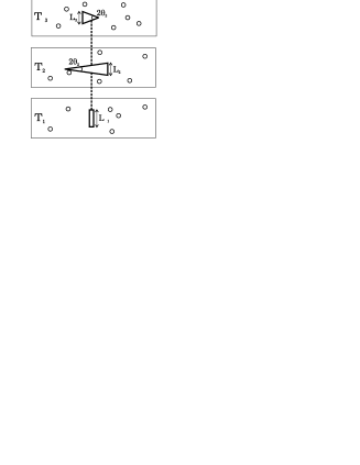
Figure 5: Construction of a thermal Brownian motor with $3$ reservoirs. The three motor units are rigidly linked and move as one single entity.

One may wonder what is the effect of the addition of a reservoir that is at equilibrium with a motor consisting of two units (at lowest order in $\varepsilon$). More precisely, consider $T_{1}$ to be equal to the effective temperature of reservoirs $2$ and $3$, $T_{1}={(\gamma_{2}T_{2}+\gamma_{3}T_{3})}/{(\gamma_{2}+\gamma_{3})}$. We find from Eq. (15):

$$V_{0} = \frac{\sqrt{2\pi mk_{B}}}{4M}\frac{\rho_{2}S_{2}(T_{2}-T_{1})\langle\sin^{3}{\theta}\rangle_{{}_{2}}+\rho_{3}S_{3}(T_{3}-T_{1})\langle\sin^{3}{\theta}\rangle_{{}_{3}}}{\sum_{i=1}^{3}\rho_{i}S_{i}\sqrt{T_{i}}\langle\sin^{2}{\theta}\rangle_{{}_{i}}}.$$ (27)

We conclude that the presence of motor unit $1$ slows down the systematic speed. Its single effect is the addition of an extra friction term, cf. the denominator in the above formula.

5 Efficiency

As pointed out in the introduction, the efficiency of a thermal motor, like the one discussed here, has to be compared with that of a Carnot engine. The fact that we can extract work by adding a load to the motor implies that there must be a concomitant transfer of energy from the hot to the cold reservoir. A fundamental difference with the Carnot construction is however that the motor is at all times simultaneously in contact with both the thermal reservoirs (we consider for simplicity the case of two reservoirs). As a result, we expect that the object will acquire a temperature intermediate between $T_{1}$ and $T_{2}$. This observation is confirmed by the calculations mentioned above, where it is found that, to lowest order in $\varepsilon$, the velocity distribution of the motor is Gaussian at an effective temperature $T_{\mathrm{eff}}$ given by Eq. (14). At this order of perturbation, one can easily evaluate the corresponding heat flux between the reservoirs and show that it obeys a Fourier law, see below. Furthermore, it has been a matter of debate whether this irreversible entropy producing process is reducing (dramatically) the efficiency of the motor as a thermal engine. We will not discuss this matter further, see [11], [12], [13] and [4] for more details . We rather focus on a more practical definition of efficiency, namely the one considered in finite time thermodynamics. Indeed, in practical applications, Carnot efficiency is a less relevant quantity, since the central issue is not work but power. Hence, we will evaluate the efficiency of the Brownian motor at maximum power. To do so, we have to repeat the above analysis but including an explicit calculation of the heat flux and applying a (constant) load force $F$ to the motor.

5.1 Heat conduction

To explicitly include the energy transfer between the heat reservoirs, we add in the Boltzmann-Master equation, an additional variable $E_{1}$ corresponding to the energy (change) in reservoir $1$. Adding the direct acceleration produced by the external force, we obtain the following equation for the probability density $P(V,E_{1},t)$ (prime is denoting precollisional values):

$$\partial_{t}P(V,E_{1},t) = \int dV^{\prime}W_{1}(V|V^{\prime})P(V^{\prime},E_{1}^{\prime},t)-\int dV^{\prime}W_{1}(V^{\prime}|V)P(V,E_{1},t)$$ (28)

$$+\int dV^{\prime}W_{2}(V|V^{\prime})P(V^{\prime},E_{1},t)-\int dV^{\prime}W_{2}(V^{\prime}|V)P(V,E_{1},t)$$

$$-\frac{\partial}{\partial V}\left(\frac{F}{M}P(V,E_{1},t)\right),$$

with $W(V^{\prime}|V)=\sum_{i}W_{i}(V^{\prime}|V)$ the transition probability per unit time for the motor to go from speed $V^{\prime}$ to $V$, given by Eq. (3). Conservation of energy in reservoir $1$ implies

$$\frac{1}{2}MV^{2}+E_{1} = \frac{1}{2}MV^{\prime 2}+E_{1}^{\prime}.$$ (29)

For the transition probability $W_{i}(V;r)\equiv W_{i}(V^{\prime}|V)$ with jump amplitude $r=V^{\prime}-V$, the conservation of energy permits us to rewrite the above equation as:

$$\partial_{t}P(V,E_{1},t) = \int drW_{1}(V-r;r)P(V-r,E_{1}+\frac{1}{2}Mr(2V-r),t)$$ (30)

$$-\int drW_{1}(V;r)P(V,E_{1},t)$$

$$+\int drW_{2}(V-r;r)P(V-r,E_{1},t)-\int drW_{2}(V;r)P(V,E_{1},t)$$

$$-\frac{\partial}{\partial V}\left(\frac{F}{M}P(V,E_{1},t)\right).$$

Equivalently, we have:

$$\partial_{t}P(V,E_{1},t)=\int dr\left[e^{-r\frac{\partial}{\partial V}}e^{\frac{Mr}{2}(2V+r)\frac{\partial}{\partial E_{1}}}-1\right]W_{1}(V;r)P(V,E_{1},t)$$

$$+\left[e^{-r\frac{\partial}{\partial V}}-1\right]W_{2}(V;r)P(V,E_{1},t)-\frac{\partial}{\partial V}\left(\frac{F}{M}P(V,E_{1},t)\right).$$ (31)

Since $\langle E_{1}\rangle=\int dV\int dE_{1}E_{1}P(V,E_{1},t)$, the energy exchange between the reservoirs obeys the following equation:

$$\partial_{t}\langle E_{1}\rangle=\int dr\int dV\int dE_{1}E_{1}\left\{\left[\sum_{n=0}^{\infty}\frac{(-r)^{n}}{n!}\frac{\partial^{n}}{\partial V^{n}}\sum_{m=0}^{\infty}\frac{(\frac{Mr}{2}(2V+r))^{m}}{m!}\frac{\partial^{m}}{\partial E_{1}^{m}}-1\right]W_{1}(V;r)\right.$$

$$+\left.\left[\sum_{n=0}^{\infty}\frac{(-r)^{n}}{n!}\frac{\partial^{n}}{\partial V^{n}}-1\right]W_{2}(V;r)-\frac{\partial}{\partial V}\frac{F}{M}\right\}P(V,E_{1},t).$$ (32)

The only non-vanishing contribution comes from the term $n=0,m=1$, whence

$$\partial_{t}\langle E_{1}\rangle = -\langle\int dr\frac{Mr}{2}(2V+r)W_{1}(V;r)\rangle.$$ (33)

Using the jump moments $a_{n,i}(V)$ defined by Eq. (6), we can write for the heat flux from reservoir 1 to reservoir 2:

$$\dot{Q}_{1\rightarrow 2}=-\partial_{t}\langle E_{1}\rangle = M\langle Va_{1,1}(V)\rangle+\frac{M}{2}\langle a_{2,1}(V)\rangle.$$ (34)

Again, the functions $a_{1,1}$ and $a_{2,1}$, cf. Eqs. (9)-(10), can be expanded in terms of $\varepsilon=\sqrt{m/M}$ to find the corresponding expansion for the heat flux in the limit of large mass $M$. To lowest order, one finds that the energy flux obeys a Fourier law

$$\dot{Q}_{1\rightarrow 2}=\kappa(T_{1}-T_{2})+O\left(\frac{1}{M^{2}}\right),$$ (35)

with

$$\kappa=\frac{k_{B}}{M}\frac{\gamma_{1}\gamma_{2}}{\gamma_{1}+\gamma_{2}}.$$ (36)

5.2 Power

The time evolution for the average speed obtained from the Boltzmann equation (28),

$$\partial_{t}\langle V\rangle = \langle a_{1}(V)\rangle+\frac{F}{M},$$ (37)

differs from Eq. (7) by the acceleration resulting from the addition of the force $F$. To lowest order in $\varepsilon$, the steady state solution of Eq. (8) for the second moment is unaffected by $F$ (i.e., $M\langle V^{2}\rangle=k_{B}T_{\mathrm{eff}}$) and we find that

$$\langle a_{1}(V)\rangle=-\frac{\gamma}{M}(\langle V\rangle-V_{0}).$$ (38)

Here is $\gamma$ the friction coefficient, cf. Eq. (12), and $V_{0}$ the average steady state velocity in absence of an external force, see Eq. (15). The steady-state solution of Eq. (37) thus reads:

$$\langle V\rangle = V_{0}+\frac{F}{\gamma}.$$ (39)

Note that $F_{stop}=-\gamma V_{0}$ is the stopping force (at this order of perturbation). Obviously, in order to extract work from the Brownian motor we need to apply a force smaller than $F_{stop}$. In particular one has that $F\sim 1/M$.

One defines the efficiency of the motor as the delivered work per unit time over the heat exchange per unit time (for simplicity, we assume from here on that $T_{1}>T_{2}$)

$$\eta = \frac{P}{\dot{Q}_{1\rightarrow 2}}=\frac{-F\langle V\rangle}{\dot{Q}_{1\rightarrow 2}}.$$ (40)

Since to lowest order of the perturbation in $\varepsilon$ the heat flux is not influenced by an external constant force $F$, we can maximize the efficiency by maximizing the power $-F\langle V\rangle$. One easily verifies that the latter is maximal when we apply a force equal to half the stopping force, $F=-\gamma V_{0}/2$.

Shape	Fig.	Efficiency $\eta$ at maximum power
Triangula	1(a)	$\frac{\pi}{32}\frac{m}{M}(1-\sin{\theta_{0}})^{2}\frac{(\sqrt{T_{1}}-\sqrt{T_{2}})^{3}}{\sqrt{T_{1}T_{2}}(\sqrt{T_{1}}+\sqrt{T_{2}})}$
Triangulita	1(b)	$\frac{\pi}{16}\frac{m}{M}\frac{(1-\sin^{2}{\theta_{0}})^{2}}{1+\sin{\theta_{0}}}\sqrt{\frac{T_{1}}{T_{2}}}\frac{T_{1}-T_{2}}{(2\sqrt{T_{1}}+(1+\sin\theta_{0})\sqrt{T_{2}})^{2}}$
Triangle - triangle ($\rhd\lhd$)	1(c)	$\frac{\pi}{32}\frac{m}{M}(1-\sin{\theta_{0}})^{2}\frac{T_{1}-T_{2}}{\sqrt{T_{1}T_{2}}}$
Triangle - triangle ($\theta_{1}\neq\theta_{2}$)	1(d)	$\frac{\pi}{32}\frac{m}{M}(1+\sin\theta_{1})(1+\sin\theta_{2})\frac{T_{1}-T_{2}}{\sqrt{T_{1}T_{2}}}\left[\frac{\sqrt{T_{1}}(1-\sin\theta_{2})-\sqrt{T_{2}}(1-\sin\theta_{1})}{\sqrt{T_{1}}(1+\sin\theta_{1})+\sqrt{T_{2}}(1+\sin\theta_{2})}\right]^{2}$

Table 2: Analytic result for the lowest order contribution to the efficiency $\eta$ at maximum power, in the situation of equal densities in the reservoirs ($\rho_{1}=\rho_{2}$, $T_{1}>T_{2}$).

The resulting efficiency of the thermal engine at maximum power is then given by:

$$\eta=\frac{M}{4k_{B}}\frac{(\gamma_{1}+\gamma_{2})^{2}}{\gamma_{1}\gamma_{2}}\frac{V_{0}^{2}}{T_{1}-T_{2}}.$$ (41)

One can immediately deduce from Eqs. (12) and (15), that the efficiency $\eta$ is very low, due to a prefactor $m/M$: for small $m/M$ the heat conductivity is the dominant factor and both the rectified motion and resulting work are a second order effect. This observation is of course restricted to our discussion of the small $\varepsilon$ limit. In fact much higher efficiencies can be in principle be achieved when one moves away from this limit [14].

Since the expression for the efficiency of an arbitrary motor, Eq. (41), is rather complex, we have reproduced the efficiency for the models of Fig. 1 in Table 2. In particular, $\eta$ simplifies significantly for identical conditions in both reservoirs (equal densities $\rho_{1}=\rho_{2}$ and equal objects $F_{1}(\theta)=F_{2}(\theta)$ and $S_{1}=S_{2}$):

$$\eta = \frac{\pi}{32}\frac{m}{M}\left(\frac{\langle\sin^{3}\theta\rangle}{\langle\sin^{2}\theta\rangle}\right)^{2}\frac{(\sqrt{T_{1}}-\sqrt{T_{2}})^{3}}{\sqrt{T_{1}T_{2}}(\sqrt{T_{1}}+\sqrt{T_{2}})}.$$ (42)

References

References

- [1] Reimann P 2002 Phys. Rep. 361 57
- [2] Reimann P, Kawai R, Van den Broeck C and Hänggi P 1999 Europhys. Lett. 45 545 Jülicher F and Prost J 1995 Phys. Rev. Lett. 75 2618
- [3] Parrondo J M R and Jiménez de Cisneros B 2002 Appl. Phys. A 75 193
- [4] Van den Broeck C, Kawai R, and Meurs P 2004 Phys. Rev. Lett. 93 090601 Van den Broeck C, Meurs P and Kawai R 2005 New J. Phys. 7 10
- [5] Meurs P, Van den Broeck C and Garcia A 2004 Phys. Rev. E 70 051109
- [6] Smoluchowski M von 1912 Physik. Zeitschr. 13 1069
- [7] Feynman R P, Leighton R B and Sands M 1963 The Feynman Lectures on Physics I (Reading: Addison-Wesley), Chapter 46.
- [8] Van Kampen N G 1981 Stochastic Processes in Physics and Chemistry (Amsterdam: North-Holland)
- [9] Onsager L 1931 Phys. Rev. 37 405 Onsager L 1931 Phys. Rev. 38 2265
- [10] Gomez-Marin A and Sancho J M 2005 Phys. Rev. E 71 021101
- [11] Parrondo J M R and Espagnol P 1996 Am. J. Phys. 64 1125
- [12] Jarzynski C and Mazonka O 1999 Phys. Rev. E 59 6448
- [13] Sokolov I M 1999 Europhys. Lett. 44 278
- [14] Van den Broeck C Thermodynamic efficiency at maximum power preprint