Flat-Bands on Partial Line Graphs
— Systematic Method for Generating Flat-Band Lattice Structures —

Abstract

We introduce a systematic method for constructing a class of lattice structures that we call “partial line graphs”. In tight-binding models on partial line graphs, energy bands with flat energy dispersions emerge. This method can be applied to two- and three-dimensional systems. We show examples of partial line graphs of square and cubic lattices. The method is useful in providing a guideline for synthesizing materials with flat energy bands, since the tight-binding models on the partial line graphs provide us a large room for modification, maintaining the flat energy dispersions.

It has been known that several novel phenomena occur in electronic systems with “flat-bands”, i.e., energy bands with flat dispersions in an entire $k$-space. Flat-band ferromagnetism is the most well-known example, and many research studies have been devoted to this subject. Mielke first proved the existence of ferromagnetism in a Hubbard model on “line graphs” [1, 2, 3]. Later, Tasaki showed rigorously the existence of ferromagnetic ground states in the so-called Tasaki model [4]. These tight-binding models have a flat-band as the lowest band. Since the single-electron states in the lowest band are completely degenerate, the ground states of noninteracting models with the half-filled lowest band are highly degenerate due to possible spin configurations. The introduction of a Hubbard interaction does not change the energy of perfectly ferromagnetic ground states since these states do not encounter on-site repulsive interactions. If the energies of other states are increased by such interactions, the so-called flat-band ferromagnetism is realized. Such a flat-band ferromagnetism can be stable against small perturbations to hopping terms [5, 6, 7]. It is known that a flat-band also appears in a tight-binding model on a bipartite lattice with different numbers of sub-lattice sites. The ground state of the half-filled Hubbard model on this type of lattice was shown to be ferrimagnetic (Lieb theorem) [8]. Motivated by these studies, several attempts at finding a flat-band ferromagnetism in real materials have been carried out. Following the guiding concept of constructing localized wave functions, tight-binding models with flat-bands were proposed in several theoretical studies [9, 10, 11, 12]. For example, in the graphite with zigzag edges, the edge states formed a flat-band and the magnetism caused by the edge band was predicted [10].

Imada and Kohno argued that a flat dispersion may enhance the pairing instabilities in the systems near a Mott insulator with a singlet ground state. According to them, the enhanced degeneracy and suppression of single-particle processes due to the flat dispersion may enhance pairing instability in doped systems, which may be the cause of the high-$T_{c}$ in cuprates [13].

In this manner, the search for tight-binding models with flat-bands is strongly desired from both theoretical and experimental points of view. Thus far, several attempts at constructing tight-binding models with a flat-band have been carried out. In most cases, we have to determine the parameters in the models as realize a localized wave function by solving the Schrödinger equation directly [11, 12]. Although a few systematic methods for constructing flat-band tight-binding models, e.g., “line graph” and “cell construction”, have been proposed [1, 2, 4], the application of these methods can be possible in certain artificial models. Thus, the number of constructed models is limited. In this paper, we introduce a new simple systematic method for constructing tight-binding models on a class of lattice structures that we call “partial line graphs” in which flat-bands emerge. We can apply this method to any two-dimensional (2D) or three-dimensional (3D) lattices. In addition, the generalization of the “partial line graphs” is also possible, which makes the flat-band stable in a wide parameter range. Such a flexibility is important as a guideline for constructing a material with a flat-band. First, we show the method for constructing a partial line graph. Several tight-binding models produced by generalizing the partial line graph also realize flat-bands. We describe the rules for the generalization and show examples of generalized partial line graphs of square and cubic lattices. Finally, we prove the realization of flat-bands in these systems.

Given a 2D or 3D lattice, we can construct its partial line graphs in the following manner. We divide the lattice into $N$ sublattices ($N>1$), where each site on a sublattice is equivalent and connected only to the sites on different sublattices. Next, we select a site of one (A) of the sublattices, which is connected to $z$ sites on different sublattices, and replace the selected site with $z$ sites (A₁, A₂, $\cdots$, A_z) created on bonds connecting the selected site to other sites. We connect A₁, A₂, $\cdots$ and A_z to each other through bonds. Repeating the same process on all the sites on the A sublattice, we construct a partial line graph of the given lattice, where the A sublattice is replaced by a lattice of clusters composed of $z$ sites. Namely, we apply the concept of the line graph only to one of the sublattices. The constructed lattice has $N+z-1$ sites within a unit cell. A tight-binding single-particle model with the same hopping amplitude $t$ on all bonds realizes flat-bands at the energy $-t$, as will be shown later.

As an example, let us consider a partial line graph of the square lattice. First, we divide the lattice into two sublattices (A and B), as shown in Fig. 1(a). We then create four sites (A₁, A₂, A₃ and A₄) on the bonds connected to the sites on the A sublattice (see Fig. 1(b)). Connecting the new sites, we obtain a partial line graph shown in Fig. 1(c), which contains five unidentical sites in the unit cell. Assuming the hopping amplitude $t$ on all bonds, we calculate the energy dispersion. The result is shown in Fig. 2(a), where doubly degenerate flat-bands exist at $E=-t$. Furthermore, all the dispersion relations along the highly symmetric lines in the ${\bf k}$-space, ${\bf k}=(0,k_{y})$ or $(k_{x},0)$, are flat, as shown in Fig. 2(a).

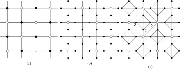
Figure 1: (a) 2D square lattice ($z=4$) with two sublattices, where A and B sublattices are shown by black and white circles, respectively. (b) All sites on the A sublattice are removed, and new sites on the bonds connected to the removed sites are created. (c) The new sites on the clusters are connected. The partial line graph of the 2D square lattice is obtained. The unit cell is shown by a dashed line.

As mentioned above, we have assumed that all the hopping amplitudes and the on-site potential energies on all sites are the same. However, a flat-band emerges in more generalized models containing different hopping amplitudes and/or on-site energies, if we choose these parameters properly. The generalized partial line graphs are constructed by the following procedures. In the following discussions, we call all the sites other than those on the A sublattice simply as B sites, although they may belong to different sublattices.

(i) The on-site energies on the B sites do not affect flat-bands at $E=-t$. For example, the value of the on-site energies of the B sites $\epsilon$ on the partial line graph of the square lattice may be arbitrary. We show the energy dispersions for $\epsilon=0.5t$ in Fig. 2(a) together with those for $\epsilon=0$.

(ii) We can take arbitrary hopping amplitudes on the bonds that connect the A and B sites or two B sites, while fixing the amplitudes within A clusters to be $t$. Flat-bands at $E=-t$ are also realized in this case. One of these models is shown in Fig. 3(a) and an example of its band dispersions is shown in Fig. 2(b).

(iii) The hopping amplitudes within A clusters can also be tuned if $z\geq N+2$. We classify $z$ sites in an A cluster into $M$ subsets (S₁, S₂, $\cdots$, S_M), where $M$ should satisfy $z-N\geq M>1$. When the hopping amplitudes between sites in the same subset and between those in the subsets $S_{i}$ and $S_{j}$ are considered to be $t_{0}$ and $t_{ij}$, respectively, the model has a flat-band at $E=-t_{0}$. For example, we divide an A cluster of the partial line graph of the 2D square lattice into two subsets, $S_{1}$ and $S_{2}$, as shown in Fig. 3(b) and assume $t_{0}=0$ and $t_{12}=t$. The band dispersions of this model with a flat-band at $E=0$ are shown in Fig. 2(c).

(iv) We can even maintain the original sites on the A sublattice, which was removed in the original partial line graphs. This type of lattice contains A clusters composed of $z+1$ sites. An example of this generalization of the 2D square lattice and its band dispersions are shown in Figs. 3(c) and 2(d), respectively. Note that applying procedure (iii) for the model in Fig. 3(c) reproduces the Lieb model [8].

Figure 2: (a) Dispersion relations for the partial line graph of the square lattice (Fig. 1(c)). The on-site energy $\epsilon$ on the B site are considered to be $0$ and $0.5t$, while the on-site energies within four-site clusters are $0$. (b) Dispersion relations for the generalized partial line graph shown in Fig. 3(a) with $t_{1}/t=0.2$ and $t_{2}/t=0.8$. (c) Dispersion relations for the generalized partial line graph shown in Fig. 3(b). (d) Dispersion relations for the generalized partial line graph shown in Fig. 3(c).

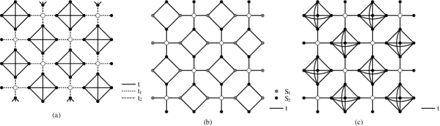
Figure 3: Generalized partial line graphs of the 2D square lattice. (a) Arbitrary hopping amplitudes from the B₁ original sublattices. (b) Generalization for the hopping amplitude within the A cluster. (c) Addition of the original site on the A cluster.

Thus far, we have shown only the examples constructed from the 2D square lattice. However, many types of tight-binding model with flat-bands can be constructed systematically by applying the above-mentioned procedures and their combinations to any type of lattice structure. As an example of 3D models, we introduce a generalized partial line graph of a 3D cubic lattice (Fig. 4(a)) and show its dispersion relations in Fig. 4(b). In this case, flat-bands appear at $E=0$ and $-2t$.

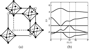
Figure 4: (a) Generalized partial line graph of a 3D cubic lattice, where all hopping amplitudes on the bonds are assumed to be $t$. (b) Dispersion relation.

Let us now prove the existence of flat-bands. We prove first that flat-bands emerge at $E=-t$ on an original partial line graph. Electronic states are described using the Bloch wave function $\phi_{\bf k}$ with the wave vector ${\bf k}$:

$$\phi_{\bf k} =\sum_{R} \left[b_{1\,{\bf k}}\phi_{{\rm B}\,1}({\bf R})+\cdots+b_{N-1\,{\bf k}}\phi_{{\rm B}\,N-1}({\bf R})\right.$$ (1)

$$\left.+a_{1\,{\bf k}}\phi_{{\rm A}\,1}({\bf R})+\cdots+a_{z\,{\bf k}}\phi_{{\rm A}\,z}({\bf R})\right]e^{i{\bf k}\cdot{\bf R}},$$

where the wave functions $\phi_{{\rm A}\,1},\cdots,\phi_{{\rm A}\,z}$ represent the atomic states within A clusters, and those on B sites are given by $\phi_{{\rm B}\,1},\cdots,\phi_{{\rm B}\,N-1}$. The wave function $\phi_{\bf k}$ for the energy $E_{\bf k}$ satisfies the eigenvalue equation ${\cal H}\phi_{\bf k}=E_{\bf k}\phi_{\bf k}$. The Hamiltonian ${\cal H}$ for the wavevector ${\bf k}$ is represented by an $(N+z-1)\times(N+z-1)$ matrix, which can be written as

$${\cal H}=\left(\begin{array}[]{cc}\cal{B}({\bf k})&\cal{G}({\bf k})\\ \cal{G}^{\dagger}({\bf k})&\cal{T}\end{array}\right).$$ (2)

Here, ${\cal B}({\bf k})$ and ${\cal G}({\bf k})$ are the $(N-1)\times(N-1)$ and $(N-1)\times z$ block matrices, respectively. The $z\times z$ block matrix $\cal{T}$ is independent of the wave vector ${\bf k}$, and all matrix elements, except the diagonal elements, are $t$:

$${\cal T}=\left(\begin{array}[]{cccc}0&t&\cdots&t\\ t&0&\cdots&t\\ \vdots&\vdots&\ddots&\vdots\\ t&t&\cdots&0\end{array}\right).$$ (3)

Assume that the eigenfunction $\phi_{f\,{\bf k}}$ for the eigenvalue $-t$ has no amplitude on B sites, i.e., $b_{i\,{\bf k}}=0$ for $1\leq i\leq N-1$ in eq.(1). Then, all $z$ equations $({\cal T}+tI)\ ^{\rm t}(a_{1\,{\bf k}},a_{2\,{\bf k}},\cdots,a_{z\,{\bf k}})=0$ are identical, and the eigenvalue equation is reduced to $N$ independent linear equations for the unknown $z$ coefficients $a_{1\,{\bf k}},a_{2\,{\bf k}},\cdots,a_{z\,{\bf k}}$:

$${\cal G}({\bf k})\ ^{\rm t}(a_{1\,{\bf k}},a_{2\,{\bf k}},\cdots,a_{z\,{\bf k}}) = 0,$$ (4)

$$a_{1\,{\bf k}}+a_{2\,{\bf k}}+\cdots+a_{z\,{\bf k}} = 0.$$ (5)

Hence, we obtain $z-N$ independent solutions for $z$ unknowns if the condition $z>N$ is satisfied. That is, we have $z-N$-fold degenerate energy bands at $E_{\bf k}=-t$, whose dispersions are flat in the entire ${\bf k}$ space. For any wave vectors $k$, by making nodes on B sites, a wave function takes the eigenvalue $-t$.

It is obvious that the flat-bands at $E=-t$ do not depend on the on-site energy on the B sites and the hopping amplitudes from/to the B sites, since they modify only eq. (4) and do not change the number of independent equations. Thus, once all the on-site energies in the A clusters are identical, we can choose an on-site energy on the B sites and an arbitrary amplitude from/to the B sites to realize flat-bands, as was already illustrated for the 2D square lattice in Figs. 2(a) and 2(b).

In generalization (iii), we tune the hopping amplitudes within an A cluster by dividing the cluster into $M$ subsets {$S_{1},S_{2},\cdots,S_{M}$} and taking the hopping amplitudes in the same subsets to be $t_{0}$ and those between the subset $S_{i}$ and $S_{j}$ to be $t_{ij}$. We prove that flat-bands emerge at $E=-t_{0}$. In this case the block matrix ${\cal T}$ in eq. (2) is written as

$${\cal T}=\left(\begin{array}[]{cccc}{\cal T}_{0}&{\cal T}_{1\,2}&\cdots&{\cal T}_{1\,M}\\ {\cal T}_{2\,1}&{\cal T}_{0}&\cdots&{\cal T}_{2\,M}\\ \vdots&\vdots&\ddots&\vdots\\ {\cal T}_{M\,1}&{\cal T}_{M\,2}&\cdots&{\cal T}_{0}\end{array}\right),$$ (6)

where

$${\cal T}_{0}=\left(\begin{array}[]{cccc}0&t_{0}&\cdots&t_{0}\\ t_{0}&0&\cdots&t_{0}\\ \vdots&\vdots&\ddots&\vdots\\ t_{0}&t_{0}&\cdots&0\end{array}\right),$$ (7)

and

$${\cal T}_{ij}=\left(\begin{array}[]{ccc}t_{ij}&\cdots&t_{ij}\\ \vdots&\ddots&\vdots\\ t_{ij}&\cdots&t_{ij}\end{array}\right).$$ (8)

If we assume the eigenfunction $\phi_{fk}^{\prime}$ with no amplitudes on B sites for the eigenvalue $-t_{0}$, the equation $({\cal T}+t_{0}I)(a_{1\,k},a_{2\,k},\cdots,a_{z\,k})^{t}=0$ is transformed to $M$ independent equations:

$$t_{0}A_{1}+t_{1\,2}A_{2}+\cdots+t_{1\,M}A_{M} = 0$$ (9)

$$t_{2\,1}A_{1}+t_{0}A_{2}+\cdots+t_{2\,M}A_{M} = 0$$ (10)

$$\vdots\hskip 56.9055pt$$

$$t_{M\,1}A_{1}+t_{M\,2}A_{2}+\cdots+t_{0}A_{M} = 0,$$ (11)

where

$$A_{m}=\sum_{i\in S_{m}}a_{i\,{\bf k}}.$$ (12)

By adding eq. (4), we obtain $N+M-1$ independent equations for $z$ unknowns, which leads to $z-N-M+1$-fold degenerate flat-bands at $E=-t_{0}$. The examples with $t_{0}=0$, which result in flat-bands at $E=0$, are shown in Figs. 3(b) and 4 (a). It is interesting to note that in the 3D example (Fig. 4(a)), another flat-band appears at $E=-2t$. This is a unique feature of the model where the hopping amplitudes $t_{ij}$ between the subsets $S_{i}$ and $S_{j}$ are independent of $i$ and $j$, and $M=3$.

Finally, let us prove generalization (iv). Here, we maintain the original sites on the A sublattice, which has been eliminated on the partial line graphs. Even in this lattice, we may assume the wave function $\phi_{fk}$, which has no amplitudes on B sites for the eigenvalue $-t$. Then we have $N$ independent equations for $z+1$ unknowns, and can determine the $z-N+1$ independent solutions. Thus, there are flat-bands at $E=-t$ with $z-N+1$-fold degeneracy.

In this paper, we have introduced a systematic method for constructing tight-binding models on generalized partial line graphs with flat energy bands. We have shown above only examples for the lattices divided originally into two sublattices. However, we can apply the method to the lattices with any number of sublattices. One realizes that the combinations of the described generalizations are numerous and useful for generating flat-band models. Since the flatness of the dispersion may lead to instabilities in the presence of interactions, it is important to study the many-body effects of the electrons on the generalized partial line graphs. For example, the ground state with a half-filled flat-band can be a partially polarized ferromagnetic state. It might be obvious that a ferrimagnetic state is a ground state in some of the generalized partial line graphs of Fig. 3(c), since one of them is the Lieb lattice, where it is proven rigorously that the ground state is a ferrimagnetic state. On the other hand, it is well known that the fully polarized state on the flat-band $|\Psi\rangle$ is the unique ground state, when the flat-band is the lowest (highest) energy band and the single-particle density matrix $\rho_{xy}\propto\langle\Psi|c^{\dagger}_{x\uparrow}c_{y\uparrow}|\Psi\rangle$ is irreducible [3]. Although the energy eigenvalue of the flat-band in the partial line graphs is not the lowest (highest), such a partially polarized ferromagnetic state can be a ground state when the band gaps on both sides of the flat-band exist for $U/t\ll 1$ [3]. In fact, in a chain of square models, where a flat-band can be isolated, a flat-band ferromagnetism is realized for small $U/t$ with appropriate parameters [14]. Since we can isolate a flat-band by tuning the parameters as shown in Fig2. 2(b) and 2(d), a partially polarized ferromagnetic state can be a ground state in certain generalized partial line graphs.

We expect that the method is also useful in providing a guideline for synthesizing materials with flat-bands, since there is a large room for modifying the models. We can vary on-site energies, hopping amplitudes, and other parameters, while maintaining the flat-bands. Such flexibility is important in the view point of material designing. The fact that the on-site energies on B sites do not affect the flatness of the dispersion is particularly important. This fact indicates that the atomic species on B sites can be different from those in A clusters in a realistic system. Thus, we may expect that a generalized partial line graph may be realized in certain compounds. As a candidate, we expect that the quasi-one-dimensional lattice shown in Fig. 3(a), the 2D one in Fig. 3(b), and the 3D one in Fig. 4(a) will be realized in real materials. It is also useful that the position of the flat-band can be tuned by changing the hopping amplitudes, which indicates that the position of the flat-band can be moved toward the Fermi level without changing the carrier density by applying (chemical) pressure to the material. A clusters can be considered as $z$-fold degenerate orbitals as treated in refs. nishino03 and nishino05, which is also useful in the view point of material designing.

This work is supported by a Grant-in Aid from the Ministry of Education, Culture, Sports, Science and Technology of Japan.

References

- [1] A. Mielke: J. Phys. A 24 (1991) 3311.
- [2] A. Mielke: J. Phys. A 25 (1992) 4335.
- [3] A. Mielke: Phys. Lett. A 174 (1993) 443.
- [4] H. Tasaki: Phys. Rev. Lett. 69 (1992) 1608.
- [5] K. Kusakabe and H. Aoki: Phys. Rev. Lett. 72 (1994) 144.
- [6] H. Tasaki: Phys. Rev. Lett. 73 (1994) 1158.
- [7] H. Tasaki: Phys. Rev. Lett. 75 (1995) 4678.
- [8] E. H. Lieb: Phys. Rev. Lett. 62 (1989) 893.
- [9] N. Shima and H. Aoki: Phys. Rev. Lett. 71 (1993) 4389.
- [10] M. Fujita, K. Wakabayashi, K. Nakada and K. Kusakabe: J. Phys. Soc. Jpn. 66 (1996) 1920.
- [11] S. Nishino, M. Goda and K. Kusakabe: J. Phys. Soc. Jpn. 72 (2003) 2015.
- [12] S. Nishino and M. Goda: J. Phys. Soc. Jpn. 74 (2005) 393.
- [13] M. Imada and M. Kohno: Phys. Rev. Lett. 84 (2000) 143.
- [14] R. Arita, K. Kuroki, H. Aoki, A. Yajima and M. Tsukada: Phys. Rev. B 57 (1998) 6854.