The spherical $2+p$ spin glass model: an analytically solvable model with a glass-to-glass transition.

Abstract

We present the detailed analysis of the spherical $s+p$ spin glass model with two competing interactions: among $p$ spins and among $s$ spins. The most interesting case is the $2+p$ model with $p\geq 4$ for which a very rich phase diagram occurs, including, next to the paramagnetic and the glassy phase represented by the one step replica symmetry breaking ansatz typical of the spherical $p$-spin model, other two amorphous phases. Transitions between two contiguous phases can also be of different kind. The model can thus serve as mean-field representation of amorphous-amorphous transitions (or transitions between undercooled liquids of different structure). The model is analytically solvable everywhere in the phase space, even in the limit where the infinite replica symmetry breaking ansatz is required to yield a thermodynamically stable phase.

Spin glasses have become in the last thirty years the source of ideas and techniques now representing a valuable theoretical background for “complex systems”, with applications not only to the physics of amorphous materials, but also to optimization and assignment problems in computer science, to biology, ethology, economy and finance. These systems are characterized by a strong dependence from the details, such that their behavior cannot be rebuilt starting from the analysis of a ’cell’ constituent but an approach involving the collective behavior of the whole system becomes necessary. One of the feature usually expressed is the existence of a large number of stable and metastable states, or, in other words, a large choice in the possible realizations of the system and a rather difficult (and therefore slow) evolution through many, details-dependent, intermediate steps, hunting its equilibrium state or optimal solution.

Mean-field models have largely helped in comprehending many of the mechanisms yielding such complicated structure and also have produced new theories (or combined among each other old concepts pertaining to other fields) such as, e.g., the spontaneous breaking of the replica symmetry and the ultrametric structure of states.

Among mean-field models spherical models are analytically solvable even in the most complicated cases. Up to now only spherical models with one step Replica Symmetry Breaking (1RSB) phases were studied, mainly due to their relevance for the fragile glass transition. KirThi87 ; CriSom92 ; REV The possibility of the existence of Full Replica Symmetry Breaking (FRSB) phases in spherical models was first pointed out by Nieuwenhuizen Nieuwenhuizen95 on the basis of the similarity between the replica free energy of some spherical models with multi-spin interactions and the relevant part of the free energy of the Sherrington-Kirkpatrick (SK) model. BraMor78 ; PytRud79 A complete analysis, however, was not provided up to now. The problem has been considered some years later CiuCri00 in connection with the possible different scenarios for the critical dynamics near the glass transition, GoeSjo89 therefore analyzing only the dynamical behavior in the 1RSB phase.

The model we present here, the $2+p$ spherical spin glass model, displays four different phases: together with the replica symmetric, the 1RSB and the FRSB phases also a new phase occurs. The evidence for the existence of such peculiar amorphous phase has been first presented in Ref. CriLeu04, and, for what concerns the organization of the states, it seems to yield the properties of a glass up to the first level of the ultrametric tree (i.e. inside and just outside a valley of the free energy landscape) and those of a spin-glass above.

Concentrating on the study of amorphous materials, in recent years some evidence has been collected for the existence of amorphous to amorphous transition (AAT), in certain glass-forming substances. One way of looking at an AAT has been to consider the kinetics of the coordination transformation occurring in strong glasses such as the vitreous Germania (GeO₂ - from fourfold to sixfold coordination rising the pressure) and Silica (SiO₂ - from tetrahedral to octahedral coordination).Tsiok98 Exactly as for the liquid-glass transition also this transition is not a thermodynamic one, but it amounts to a qualitative change of the (slow) relaxation dynamics, apparently expressing a recombination of the glass structure (see also the numerical simulations of Ref. Huang04, for a different point of view). Another kind of pressure induced AAT takes place in densified porous silicon, where the high-density amorphous Si transforms into a low density amorphous Si upon decompression.Deb01 A similar transition also takes place in undercooled water.Poole

Theoretical models have been introduced to describe an AAT. As, for instance, a model of hard-core repulsive colloidal particle subject to a short-range attractive potential that induces the particle to stick to each other. DawetAl01 ; Zac01 ; Sciorti02 In the framework of the Mode Coupling Theory (MCT) it has been shown that the interplay of the attractive and repulsive mechanisms results in the existence of a high(er) temperature “repulsive” glass, where the hard-core repulsion is responsible for the freezing in of many degrees of freedom and the kinetic arrest, and a low(er) temperature “attractive” glass that is energetically more favored than the other one but only occurs when the thermal excitation of the particles is rather small. Such theoretical and numerical predictions seem to have been successfully tested in recent experiments.Chen03 ; Eckert02 ; Pham02 Another model where AAT is found is the spherical $p$-spin model on lattice gas of Caiazzo et al. Caiazzo04 where an off-equilibrium Langevin dynamics is considered, thus going beyond the MCT assumption of equilibrium. The model we consider here might, as well, be a good mean-field representative of an amorphous-amorphous transition.

The goal of this paper is to give a detailed discussion of the different solutions describing the low temperature phase of the spherical $2+p$ spin glass model. As it happens in systems with a phase described by a 1RSB solution one must distinguish between the “static solution” obtained from the partition function and the “dynamic solution” obtained from the relaxation dynamics.KirWol87 ; CriSom92 ; CriHorSom93 To keep the length of the paper reasonable we shall consider in detail only the static approach and introduce the the dynamic solution with the help of the complexity.CriNie96 The complete dynamic approach will be presented elsewhere.

In section I we present the spherical $2+p$ spin-glass model. In section II its static behavior is studied with the help of the replica trickEA75 and the Parisi replica symmetry breaking scheme:Parisi80 four different phases occur, together with the relative transitions between them. The nature of the phases is thoroughly discussed and analytical exact solutions for order parameters, transition lines and thermodynamic functions are provided all over the parameter space. In section III the existence of an exponential number of energetically degenerate pure states is considered by analyzing the complexity function. The connection between the “marginal condition” (maximum of the complexity in free energy) and the dynamical solution leads, in section IV to the discussion of the latter in those cases where it differs from the static one. In Appendix A and B we show, respectively, the Parisi anti-parabolic equation for the $2+p$ model, and its analytical solution. In appendix C some basic features of the behavior of the much simpler $s+p$ model ($s$, $p>2$) are given.CiuCri00 ; AnetAl Eventually, in appendix D, a proof is given that no phases other than those here presented exist for the spherical $2+p$ spin glass model.

I The Model

The spherical $2+p$ spin glass model is defined by the Hamiltonian

$${\cal H}=\sum_{i<j}^{1,N}J^{(2)}_{ij}\sigma_{i}\sigma_{j}+\sum_{i_{1}<\ldots<i_{p}}^{1,N}J^{(p)}_{i_{1}\ldots i_{p}}\sigma_{i_{1}}\cdots\sigma_{i_{p}}$$ (1)

where $p$ is an integer equal or larger than $3$ and $\sigma_{i}$ are $N$ continuous real spin variables which range from $-\infty$ to $+\infty$ subject to the global spherical constraint

$$\sum_{i=1}^{N}\sigma_{i}^{2}=N.$$ (2)

The coupling strengths $J^{(p)}_{i_{1}\ldots i_{p}}$ ($p=2,3,\ldots$) are quenched independent identical distributed zero mean Gaussian variables of variance

$$\overline{\left(J^{(p)}_{i_{1}i_{2}..i_{p}}\right)^{2}}=\frac{p!\,J_{p}^{2}}{2\,N^{p-1}},\qquad i_{1}<\cdots<i_{p}.$$ (3)

The scaling with the system size $N$ ensures an extensive free energy and hence a well defined thermodynamic limit $N\to\infty$. Without loosing in generality one may take either $J_{2}$ or $J_{p}$ equal to $1$ since this only amounts in a rescaling of the temperature $T$. To keep the discussion as simple as possible in this paper we shall not consider the effect of an external field coupled linearly with the spin variables $\sigma_{i}$.

The properties of the model strongly depend on the value of $p$. For $p=3$ the model reduces to the usual spherical $p$-spin spin glass model in a fieldCriSom92 with a low temperature phase described by a 1RSB solution. For $p>3$ the model exhibits different low temperature phases which, depending on the temperature and the ratio $J_{p}/J_{2}$ between the strength of the non-harmonic and the harmonic parts of the Hamiltonian, are described by 1RSB and/or FRSB solutions.

II The Static Solution

The static solution is obtained from the minimum of the free-energy functional computed from the partition function. The model contains quenched disorder and hence the partition function must be computed for fixed disorder realization:Ma76 ; MPV87 ; Fischer91

$$Z_{N}[{\bm{J}}^{(2)},\bm{J}^{(p)}]=\mbox{Tr}_{\sigma}\,\exp\bigl{(}-\beta{\cal H}[\bm{J}^{(2)},\bm{J}^{(p)};\sigma]\bigr{)}$$ (4)

with $\beta=1/T$. We have explicitly shown the dependence of the Hamiltonian on the realization of the random couplings to stress that $Z_{N}$ is itself a function of the couplings realization. The trace over the spins is defined as:CriSom92

$$\mbox{Tr}_{\sigma}\equiv 2\sqrt{N}\int_{-\infty}^{+\infty}\,\prod_{i=1}^{N}\,d\sigma_{i}\,\delta\left(\sum_{i=1}^{N}\sigma_{i}^{2}-N\right)\,$$ (5)

and includes the spherical constraint (2). As a consequence $\mbox{Tr}_{\sigma}(1)$ is equal to the surface of the $N$ dimensional sphere of radius $N^{1/2}$ and its logarithm gives the entropy of the model at infinite temperature.

The partition function $Z_{N}$ is a random variable, therefore the quenched free energy per spin is given by

$$\Phi_{N}=-{1\over N\beta}\ \overline{\ln Z_{N}[{\bm{J}}^{(2)},\bm{J}^{(p)}]}$$ (6)

where here, and in the following, $\overline{(\cdots)}$ denotes the average over the realizations of all couplings in the Hamiltonian:

$${\overline{(\cdots)}}=\int d{\cal P}[\bm{J}^{(2)}]\,d{\cal P}[\bm{J}^{(p)}]\,(\cdots)$$ (7)

The thermodynamic limit $N\to\infty$ of the free energy $\Phi=\lim_{N\to\infty}\Phi_{N}$ is well defined and is equal to the limit $-\lim_{N\to\infty}\ln Z_{N}[\bm{J}^{(2)},\bm{J}^{(p)}]\,/\,N\beta$ for almost all coupling realizations (self-average property).

The analytic computation of the quenched free energy, i.e., of the average of the logarithm of the partition function, is quite a difficult problem, even in simple cases as nearest neighbor one dimensional models. Since the integer moments $\overline{Z_{N}^{n}}$ of the partition function are easier to compute, the standard method to evaluate (6) uses the so called “replica trick” by considering the annealed free energy $\Phi(n)$ of $n$ non-interacting identical ‘replicas’ of the system,SKPRL75 ; MPV87 ; Fischer91

$$\Phi(n)=-\lim_{N\to\infty}{1\over N\beta n}\ \ln\overline{(Z_{N}[\bm{J}^{(2)},{\bm{J}}^{(p)}])^{n}}.$$ (8)

The quenched free energy $\Phi$ is then recovered as the continuation of $\Phi(n)$ down to the unphysical limit $n=0$,note21

$$\Phi=-\lim_{N\to\infty}\lim_{n\to 0}{\overline{(Z_{N}[J^{(2)},J^{(p)}])^{n}}-1\over N\beta n}=\lim_{n\to 0}\Phi(n).$$ (9)

In the last equality we assumed that the replica limit $n\to 0$ and the thermodynamic limit $N\to\infty$ can be exchanged. The existence of such a limit has been recently rigorously proved.Talagrand ; Guerra

The replica method gives a simple way of performing the disorder average, at the expenses of introducing an effective interaction among different replicas in the $n$-dimensional replica space. The interested reader can find a detailed presentation of the replica method for disordered systems in Refs. [MPV87, ] and [Fischer91, ] and for the particular case of spherical models in Ref. [CriSom92, ].

Applying the replica method the integer moments of the partition function of the spherical $2+p$ spin glass model can be written, neglecting all unnecessary constants and terms irrelevant for $N\to\infty$, as:CriSom92

$$\overline{Z_{N}^{n}}={\rm e}^{nNs(\infty)}\,\int_{\bm{q}>0}\prod_{\alpha<\beta}\,dq_{\alpha\beta}\ {\rm e}^{NG[\bm{q}]}$$ (10)

where $s(\infty)=(1+\ln 2\pi)/2$ is the entropy per spin at infinite temperature and $G[\bm{q}]$ the functional:

$$G[{\bm{q}}] = \frac{1}{2}\sum_{\alpha\beta}^{1,n}g(q_{\alpha\beta})+\frac{1}{2}\ln\det{\bm{q}}$$ (11)

$$g(x) = \frac{\mu_{2}}{2}x^{2}+\frac{\mu_{p}}{p}x^{p}.$$ (12)

with $\mu_{p}=(\beta J_{p})^{2}p/2$. We also introduce the two additional functions

$$\Lambda(x)=\frac{d}{dx}\,g(x),\quad\Sigma(x)=\frac{d}{dx}\,\Lambda(x)$$ (13)

whose utility will be clear in a short while.

The symmetric $n\times n$ real matrix $q_{\alpha\beta}$ is the replica overlap matrix

$$q_{\alpha\beta}=\frac{1}{N}\sum_{i=1}^{N}\,\sigma_{i}^{\alpha}\,\sigma_{i}^{\beta},\quad\alpha,\beta=1,\ldots,n.$$ (14)

The spherical constraint, Eq. (2), implies that the diagonal elements of the matrix $\bm{q}$ are all equal to one: $q_{\alpha\alpha}=\overline{q}=1$.

In the thermodynamic limit $N\to\infty$ the integrals in (10) can be evaluated by the saddle point method and the quenched free energy per spin $\Phi$ reads:

$$-\beta\Phi=s(\infty)+\lim_{n\to\ 0}\frac{1}{n}G[{\bm{q}}]$$ (15)

where $G[\bm{q}]$ must be evaluated on the solution of the saddle point equation which, in the $n\to 0$ limit, reads:

$$\Lambda(q_{\alpha\beta})+({\bm{q}}^{-1})_{\alpha\beta}=0,\qquad\alpha\not=\beta.$$ (16)

Stability of the saddle point calculation requires that the quadratic form

$$-\sum_{\alpha\beta}\,\Sigma(q_{\alpha\beta})\,(\delta q_{\alpha\beta})^{2}+\mbox{Tr}({\bm{q}}^{-1}\,\delta{\bm{q}})^{2}$$ (17)

must be positive definite. Here above $\delta{\bm{q}}_{\alpha\beta}=\delta q_{\alpha\beta}\,(=\delta q_{\beta\alpha})$ is the fluctuation of $q_{\alpha\beta}$ from the saddle point value (16). Details of the derivation of these equations can be found in Ref. [CriSom92, ].

The structure of the overlap matrix $q_{\alpha\beta}$ reflects the organization of the different thermodynamic states, called pure states, in which each replica can be found. This however does not follow from the replica calculation and therefore to evaluate explicitly $G[{\bm{q}}]$ some ansatz on the structure of $\bm{q}$ must be imposed.

II.1 The Replica Symmetric Solution (RS)

The simplest ansatz is the one in which all replicas are in the same pure state, so that $q_{\alpha\beta}$ cannot depend on the replica indexes:

$$q_{\alpha\beta}=(1-q)\delta_{\alpha\beta}+q.$$ (18)

This is called the Replica Symmetric (RS) ansatz. This assumption is reasonable for coupling strengths not too large or high temperatures, i.e., $\mu_{2}$ and $\mu_{p}$ small enough. In both cases, indeed, the system can explore almost the whole available phase space so that different replicas will be found in the same pure state.

Inserting the RS form (18) of $q_{\alpha\beta}$ into Eq. (11) one gets

$$2\lim_{n\to 0}\frac{1}{n}\,G[{\bm{q}}]=g(1)-g(q)+\ln(1-q)+\frac{q}{1-q}$$ (19)

where $q$ is the solution of the RS saddle point equation

$$\Lambda(q)-\frac{q}{(1-q)^{2}}=\mu_{2}q+\mu_{p}q^{p-1}-\frac{q}{(1-q)^{2}}=0.$$ (20)

In absence of external fields the saddle point equation always admits the “paramagnetic” solution $q=0$. However since $q/(1-q)^{2}$ diverges as $q\to 1$ and vanishes for $q=0$ for particularly chosen values of the parameters $\mu_{p}$ and $\mu_{2}$ there may also be solutions with $0<q<1$.

The RS solution is stable, i.e. the quadratic form (17) is positive definite for $n\to\ 0$, provided that the eigenvaluenote7

$$\Lambda_{1} = -\Sigma(q)+\frac{1}{(1-q)^{2}}$$ (21)

$$= -\mu_{2}-\mu_{p}(p-1)q^{p-2}+\frac{1}{(1-q)^{2}}$$

is positive. If $q\not=0$ then dividing the saddle point equation (20) by $q$ and adding the result to (21) one gets that the requirement $\Lambda_{1}>0$ is equivalent to

$$-\mu_{p}(p-2)\,q^{p-2}>0.$$ (22)

This inequality cannot be satisfied for any $q>0$, thus we are left with the $q=0$ solution only.

For $q=0$ the eigenvalue $\Lambda_{1}$ reduces to $\Lambda_{1}=1-\mu_{2}$. Therefore, in the $(\mu_{p},\mu_{2})$ plane the paramagnetic RS solution $q=0$ is stable everywhere below the $\mu_{2}=1$ line, which represents the De Almeida-Thouless lineAT of the model.

The instability of the paramagnetic solution is due to the presence of the quadratic term in the Hamiltonian. If this is missing, as for example in the spherical $3+p$ spin glass model in which the two-body interaction is replaced by a three-body interaction, the paramagnetic solution is stable everywhere in the phase space, similarly to what happens for the spherical $p$-spin model without a field.CriSom92

II.2 The One Step Replica Symmetry Breaking Solution (1RSB)

The stability of the RS solution $q=0$ does not depend on $\mu_{p}$. However, from the analogies with the spherical $p$-spin spin glass model we expect that for $\mu_{p}$ large enough a solution with a non vanishing order parameter of the 1RSB type might lead to a thermodynamically more favorable phase.

The 1RSB solution corresponds to group the $n$ replicas into $n/m$ clusters of $m$ replicas. Any two replicas $\alpha\not=\beta$ within the same cluster have overlap $q_{1}$, whereas replicas in different clusters have overlap $q_{0}<q_{1}$. As a consequence the $n\times n$ ${\bm{q}}$ matrix breaks down into $(n/m)\times(n/m)$ blocks of dimension $m\times m$. If the element $q_{\alpha\beta}$ with $\alpha\not=\beta$ belongs to one of the diagonal block then $q_{\alpha\beta}=q_{1}$, otherwise $q_{\alpha\beta}=q_{0}$. The overlap matrix for the 1RSB ansatz can be conveniently written as:

$$q_{\alpha\beta}=(1-q_{1})\,\delta_{\alpha\beta}+(q_{1}-q_{0})\,\epsilon_{\alpha\beta}+q_{0}$$ (23)

where the matrix ${\bm{\epsilon}}$ is defined as

$$\epsilon_{\alpha\beta}=\left\{\begin{array}[]{ll}1&\mbox{if $\alpha$ and $\beta$ are in a diagonal block}\\ 0&\mbox{otherwise}\\ \end{array}\right.$$ (24)

By plugging this form of $q_{\alpha\beta}$ into the Eq. (11) one obtains:

$$2\lim_{n\to 0}\frac{1}{n}G[{\bm{q}}] = g(1)-g(q_{1})+m\,[g(q_{1})-g(q_{0})]$$ (25)

$$+\frac{q_{0}}{\chi(q_{0})}+\frac{1}{m}\,\ln\chi(q_{0})$$

$$+\frac{m-1}{m}\,\ln\chi(q_{1}).$$

where, for later convenience, we have definednote9

$$\chi(q_{1}) = 1-q_{1}$$ (26)

$$\chi(q_{0}) = 1-q_{1}+m\,(q_{1}-q_{0}).$$ (27)

The saddle point equations for $q_{0}$ and $q_{1}$ in the limit $n\to 0$, obtained either from (16) or directly from stationarity of (25) with respect to variations of $q_{0}$ and $q_{1}$, read

$$\Lambda(q_{0}) - \frac{q_{0}}{\chi(q_{0})^{2}}=0$$ (28)

$$\Lambda(q_{1}) - \Lambda(q_{0})-\frac{q_{1}-q_{0}}{\chi(q_{1})\,\chi(q_{0})}=0$$ (29)

The solution of these equations depends on the value of $m$ that, in the limit $n\to 0$, is restricted to the interval $0\leq m\leq 1$. In principle any value of $m$ which leads to a stable 1RSB solution can be chosen. However in the spirit of the saddle point calculation performed to evaluate the free energy we choose for any value of $\mu_{p}$’s the value of $m$ which minimize the functional $G[{\bm{q}}]$.note4 This leads to the additional equation

$$g(q_{1})-g(q_{0}) + \left[\frac{1}{m\,\chi(q_{0})}-\frac{q_{0}}{\chi(q_{0})^{2}}\right]\,(q_{1}-q_{0})$$ (30)

$$+ \frac{1}{m^{2}}\ln\left[\frac{\chi(q_{1})}{\chi(q_{0})}\right]=0.$$

The stability analysis of the 1RSB saddle shows that in the limit $n\to 0$ the 1RSB solution is stable as long as the 1RSB eigenvaluesnote7

$$\Lambda_{1}^{(1)} = -\Sigma(q_{1})+\frac{1}{\chi(q_{1})^{2}}$$ (31)

$$\Lambda_{0}^{(3)} = -\Sigma(q_{0})+\frac{1}{\chi(q_{0})^{2}}$$ (32)

are both positive.

The saddle point equation (28) admits always the solution $q_{0}=0$. It may also have solutions with $0<q_{0}<1$, however by using arguments similar to those that lead to the inequality (22) for the RS solution, one can show that in absence of external field any 1RSB solution with $q_{0}>0$ is unstable since it has a negative $\Lambda_{0}^{(3)}$.note5

The 1RSB saddle point equations for $q_{1}$ and $m$ can be solved for any $p$ using the same procedure used for the spherical $p$-spin spin glass model. The first step is to obtain $g(q_{1})$ from equation (30) [with $q_{0}=0$] and divide it by $q_{1}\,\Lambda(q_{1})$. Then using the saddle point equation (29) [with $q_{0}=0$] to express $\Lambda(q_{1})$ one ends up with the equation

$$2\ \frac{g(q_{1})}{q_{1}\,\Lambda(q_{1})}=z(y)$$ (33)

where

$$z(y)=-2y\frac{1-y+\ln y}{(1-y)^{2}}$$ (34)

is the auxiliary $z$-function introduced by Crisanti and SommersCriSom92 (CS) for the solution of the spherical $p$-spin spin glass model, and

$$y\equiv\frac{\chi(q_{1})}{\chi(q_{0})}=\frac{1-q_{1}}{1-q_{1}+m\,q_{1}},\qquad 0\leq y\leq 1.$$ (35)

By using $y$ and $m$ as free parameters eqs. (29) [with $q_{0}=0$] and (33) can be solved for $(\mu_{p},\mu_{2})$. A straightforward algebra leads to:

$$\mu_{p} = \frac{p}{(p-2)}\,\frac{[1-z(y)]}{q_{1}^{p-2}(1-q_{1})(1-q_{1}+m\,q_{1})}$$ (36)

$$= \frac{p}{(p-2)}\,\frac{(1-y+m\,y)^{p}}{m^{2}y(1-y)^{p-2}}\,[1-z(y)],$$

$$\mu_{2} = \frac{1}{(p-2)}\,\frac{[p\,z(y)-2]}{(1-q_{1})(1-q_{1}+m\,q_{1})}$$ (37)

$$= \frac{(1-y+m\,y)^{2}}{m^{2}y}\,\frac{[p\,z(y)-2]}{(p-2)}.$$

By fixing the value of $m$ in the interval $[0,1]$ and varying $y$ these equations represent the parametric equations of the so called $m$-lines in the $(\mu_{p},\mu_{2})$ plane. By definition $y$ can take any value between $0$ and $1$ included, however, from Eq. (37) we see that since $z(0)=0$, $\mu_{2}$ becomes negative for $y$ sufficiently close to $0$. Setting $\mu_{2}=0$ from Eq. (37) one gets

$$p\,z(y)-2=0$$ (38)

which gives the minimum value $y_{\rm min}$ of $y$. The CS $z$-function (34) is a monotonous increasing function of $y$ varying in the range $0\leq z\leq 1$, as a consequence, $\mu_{p}$ is always non-negative.

A second condition on $y$ comes form the stability analysis of the 1RSB solution. A simple inspection shows that $\Lambda_{1}^{(1)}>\Lambda_{0}^{(3)}$ so that the condition which marks the limit of the stability of the 1RSB solutions is $\Lambda_{0}^{(3)}=0$, i.e.,

$$\mu_{2}=\frac{1}{(1-q_{1}+m\,q_{1})^{2}}$$ (39)

Using now Eq. (37) one gets the equation

$$p\,z(y)-2-(p-2)\,y=0$$ (40)

whose solution gives $y_{\rm max}$, the maximum value of $y$ for the 1RSB solution.

Both boundary values $y_{\rm min}$ and $y_{\rm max}$ are functions of $p$ only. For example, for $p=3$, we have

$$y_{\rm min}=0.354993...,\quad y_{\rm max}=1$$ (41)

while for $p=4$

$$y_{\rm min}=0.195478...,\quad y_{\rm max}=0.389571...$$ (42)

The fact that for $p=3$ the maximum is $y_{\rm max}=1$ makes the $2+3$ model different from any other $2+p$ model with $p>3$, as we shall see in a while.

From the stability condition (39) it follows that if the quadratic term in the Hamiltonian were missing, as for the already mentioned $3+p$ model, then the 1RSB solution would be stable everywhere. In the Appendices C and D we shall show that indeed in this case the 1RSB solution is the only possible non-trivial solution, besides the RS solution.

II.2.1 The Transition Lines between the Paramagnet and the 1RSB-Glass phase

To find the transition lines which bound the 1RSB phase we start by noting that the $m$-lines do not cross and that the value of $\mu_{2}$ for which the 1RSB becomes unstable increases as $m$ decreases, see Eq. (39). Moreover, all $m$-lines start from $\mu_{2}=0$. As a consequence the first $m$-line one encounters in moving from the RS phase at fixed $\mu_{2}<1$ and increasing $\mu_{p}$ is the $m$-line with $m=1$. This line, which marks the transition between the RS (paramagnetic) phase and the 1RSB (glass) phase, starts on the $\mu_{p}$ axis at the point $\mu_{p}=\mu_{p}(y_{\rm min},m=1)$ and goes up to the point $\mu_{p}=\mu_{p}(y_{\rm max},m=1)$ and $\mu_{2}=1$, as can be easily seen from Eq. (39) evaluated for $m=1$.

The transition between the RS ($q=0$) and the 1RSB ($q_{1}\not=0$, $q_{0}=0$) phases is not due to an instability but occurs because the 1RSB solution leads to a thermodynamically more favorable state. Since we are dealing with the replica trick, this means that the 1RSB solution yields a value of the free energy functional (15) larger than the RS solution.note4

This mechanism resembles that of ordinary first order transitions, and indeed the order parameter $q_{1}$ jumps discontinuously from zero to a finite value, and vice-versa, at the transition. However, the free energy remains continuous across the transition –at $m=1$ the free energies of the two solutions are equal– and no discontinuity occurs in its first derivatives.

The 1RSB solution becomes unstable when $\Lambda_{0}^{(3)}=0$. This leads to a second transition line whose parametric equation in the $(\mu_{p},\mu_{2})$ plane is obtained by setting $y=y_{\rm max}$ into eqs. (36)-(37) and varying $m$ from $1$, to $0$. For $m\to 0$ the values of both $\mu_{p}$ and $\mu_{2}$ diverge but

$$\lim_{m\to 0}\frac{\mu_{2}}{\mu_{p}}=\frac{(1-y_{\rm max})^{p-2}\,[2-(p-2)y_{\rm max}]}{(p-2)\,y_{\rm max}-p}$$ (43)

and hence the 1RSB phase does not cover the full “low temperature” phase of the model.

In Figure 1 the transition lines found so far are shown together with the $m$-lines with $m=0.7,0.5$.

Figure 1: The RS and 1RSB phases for the $2+4$ model in the $(\mu_{4},\mu_{2})$ plane. The thick lines are the transition lines between different phases.

In the figure $p=4$, but any $p>3$ leads to a qualitatively similar scenario.

The case $p=3$ is special because inserting $y=y_{\rm max}=1$ into eqs. (36)-(37) one ends up with

$$\left\{\begin{array}[]{lll}\mu_{3}&=&m\\ \mu_{2}&=&1\\ \end{array}\right.\qquad 0\leq m\leq 1$$ (44)

Along this line $q_{1}=0$, see e.g. Eq. (35), and the 1RSB solution reduces to the RS solution. We have seen that the RS solution becomes unstable for $\mu_{2}=1$ thus the critical line (44) marks the transition between the RS and the 1RSB phases. The transition is continuous in both the free energy and the order parameter $q_{1}$. The transition lines for the $2+3$ model are shown in Figure 2.

Figure 2: The phase diagram of the $2+3$ model in the $(\mu_{3},\mu_{2})$ plane. The thick lines are the transition lines between the RS and 1RSB phases. In particular the thick dashed line, the $m$-line with $m=1$, is the discontinuous transition while the horizontal thick full line is the continuous transition.

In conclusion the $2+3$ model presents only one “low temperature” phase of 1RSB type and, in this respect, is equivalent to the spherical $p$-spin spin glass model in a field.CriSom92

II.3 The One-Full Replica Symmetry Broken Solutions (1-FRSB)

From Figure 1 one clearly sees that for $p>3$ the RS and 1RSB solutions do not cover the whole phase space of the $2+p$ model. In the region where both the RS and 1RSB solutions are unstable the organization of pure states has a more complex structure which cannot be described by a simple 1RSB ansatz which groups them into $n/m$ equivalent clusters. Therefore, to describe this region one must allow for clusters of different type. To this end each one of the $n/m$ clusters is divided it into $m/m_{1}$ sub-cluster of size $m_{1}$. If the procedure is repeated $R$ times, dividing at each step the smallest clusters into yet smaller clusters, one has the $R$-RSB ansatz in which the replica symmetry is broken $R$-times. The overlap $q_{\alpha\beta}$ between two replicas depends on the number of divisions separating the offspring clusters to which the replicas $\alpha$ and $\beta$ belong from the common ancestor cluster.

A simple way proposed by ParisiParisi80 to parametrize the overlap matrix $q_{\alpha\beta}$ for $R$ steps in the replica symmetry breaking consists in dividing ${\bm{q}}$ into successive boxes of decreasing size $p_{r}$, with $p_{0}=n$ and $p_{R+1}=1$, and assigning the elements $q_{\alpha\beta}$ of the matrix ${\bm{q}}$ so that

$$q_{\alpha\beta}\equiv q_{\alpha\cap\beta=r}=q_{r},\qquad r=0,\cdots,R+1$$ (45)

with $1=q_{R+1}>q_{R}>\cdots q_{1}>q_{0}$. The notation $\alpha\cap\beta=r$ means that $\alpha$ and $\beta$ belong to the same box of size $p_{r}$ but to two distinct boxes of size $p_{r+1}<p_{r}$.

Inserting this form of $q_{\alpha\beta}$ into Eq. (11) one gets with standard manipulations

$$\frac{2}{n}\,G[{\bm{q}}] = g(1)+\sum_{r=0}^{R}\,(p_{r}-p_{r+1})\,g(q_{r})$$ (46)

$$+\ln(1-q_{R})+\sum_{t=0}^{R}\,\frac{1}{p_{r}}\,\ln\frac{\hat{q}_{r}}{\hat{q}_{r+1}}$$

where $\hat{q}_{r}$ is the Replica Fourier Transform of $q_{\alpha\beta}$,Cris ; DeDom

$$\hat{q}_{r}=\sum_{s=r}^{R+1}\,p_{s}\,(q_{s}-q_{s-1})$$ (47)

The number $R$ is arbitrary. Setting $R=0$ or $R=1$ one recovers respectively the RS and the 1RSB expressions, the latter with $m=p_{1}$, while for $R\to\infty$ one gets the $\infty$-RSB solution or Full Replica Symmetry Broken (FRSB) solution. In this limit the differences $p_{r+1}-p_{r}$ become infinitesimal and the set of overlaps $\{q_{0},...,q_{R}\}$ is replaced in the limit $n\to 0$ by a non-decreasing continuous function $q(x)$ defined on the interval $x\in[0,1]$.

The free energy functional (46) for the Parisi $R$-RSB ansatz can be conveniently expressed by using the function

$$x(q)=p_{0}+\sum_{r=0}^{R}(p_{r+1}-p_{r})\,\theta(q-q_{r})$$ (48)

which equals the fraction of pair of replicas with overlap $q_{\alpha\beta}$ less or equal to $q$. With this definition, and replacing the sums by integrals, one obtains, after a little of algebra

$$\frac{2}{n}\,G[{\bm{q}}] = \int_{0}^{1}dq~{}x(q)\,\Lambda(q)$$ (49)

$$+\int_{0}^{q_{R}}\frac{dq}{\int_{q}^{1}dq^{\prime}\,x(q^{\prime})}+\ln\left(1-q_{R}\right)$$

This expression is valid for any $R$, and hence also for the FRSB solution. In the limit $R\to\infty$, $q_{r}$ becomes continuous and we can define $q(x)$ as the inverse of $x(q)$. It can be shown that $dx(q)/dq$ gives the probability density of overlaps.Parisi79 ; Parisi80

It is easy to verify that taking for $q(x)=0$ or $q(x)=q_{1}\,\theta(x-m)$ the above functional reduces to those found with the RS and 1RSB ansatzs, respectively.note1

The FRSB solution with a continuous $q(x)$ was introduced to describe the spin-glass phase of the SK model,Parisi80 and since then it has been found in many other related models. A continuous order parameter function $q(x)$ is, however, not general enough to describe the state of the $2+p$ model with $p>3$ in the whole parameter space. From the stability analysis of the 1RSB solution we see indeed that the instability occurs because the eigenvalue $\Lambda_{0}^{(3)}$ vanishes. This eigenvalue is associated with fluctuations that involve the overlaps of one cluster as a whole with the other clusters as a whole.CriSom92 Roughly speaking these fluctuations are similar to fluctuations in the RS phase with single replicas replaced by the clusters of $m$ replicas considered as single entities. As a consequence we expect that, as it happens for the fluctuations in the RS phase, a non zero overlap $q_{0}$ between clusters would stabilize the fluctuations. The solution however cannot be of 1RSB type since we have seen that any 1RSB solution with $q_{0}\not=0$ is unstable.

Based on the analogy with the instability of RS solution with clusters playing the role of single replicas, it turns out that the correct ansatz for the $2+p$ model with $p>3$ is a mixture of 1RSB and FRSB, which we have called 1-FRSB solution,CriLeu04 described by a discontinuous order parameter function in the interval $[0,1]$ of the form

$$q(x)\Rightarrow\left\{\begin{array}[]{ll}q_{1}&\mbox{for $x>m$}\\ q(x)&\mbox{for $x<m$}\end{array}\right.$$ (50)

where $q(x)$ is a non-decreasing continuous function in the semi-open interval $x\in[0,m)$, with $\lim_{x\to m^{-}}q(x)=q_{0}<q_{1}$ and $q(0)=0$,note5 see Fig. 3. For $q_{0}=q_{1}$ one recovers the FRSB solution.note8

Figure 3: Schematic form of the order parameter function $q(x)$ in the 1-FRSB phase.

In appendix D we show that the 1-FRSB solution is the only other possible non-trivial solution, beside the 1RSB (modeling a mean-field glass) and the FRSB (modeling a spin-glass) ones, for the $2+p$ model with $p>3$. It is interesting to note that this solution also follows by solving numerically in the whole interval $[0,1]$ the Parisi equations derived from the stationarity of the functional (49) with respect to order parameter function $q(x)$, see Appendices A, B. The partial differential equation is solved numerically by means of a pseudo spectral technique, see e.g. Ref. [CLP02, ], without fixing a priori any special ansatz for $q(x)$.

The free energy functional for the 1-FRSB ansatz can be obtained either by inserting the explicit form (50) of $q(x)$ into Eq. (49), or by taking in Eq. (46) $p_{R}=m$, $q_{R}=q_{1}$, $q_{R-1}=q_{0}$ and $p_{R}-p_{R-1}$ finite as $R\to\infty$. In both cases one ends up with

$$\frac{2}{n}\,G[{\bm{q}}] = g(1)-g(q_{1})+m\,[g(q_{1})-g(q_{0})]$$ (51)

$$+\int_{0}^{q_{0}}dq\,x(q)\,\Lambda(q)+\int_{0}^{q_{0}}\frac{dq}{\chi(q)}$$

$$+\frac{m-1}{m}\ln\left(1-q_{1}\right)+\frac{1}{m}\ln\chi(q_{0})$$

where

$$\chi(q)=1-q_{1}+m\,(q_{1}-q_{0})+\int_{q}^{q_{0}}\,dq^{\prime}\,x(q^{\prime})$$ (52)

Stationarity of the free energy functional $\Phi$ with respect to $q(x)$ and $q_{1}$ leads to the 1-FRSB saddle point equations:

$$\Lambda(q)=\int_{0}^{q}\,\frac{dq}{\chi^{2}(q)},\qquad 0\leq q\leq q_{0}$$ (53)

and

$$\Lambda(q_{1})-\Lambda(q_{0})=\frac{q_{1}-q_{0}}{\chi(q_{1})\,\chi(q_{0})}.$$ (54)

Finally maximization with respect to $m$ leads to the additional equation

$$g(q_{1})-g(q_{0}) = -\left[\frac{1}{m\,\chi(q_{0})}-\Lambda(q_{0})\right](q_{1}-q_{0})$$ (55)

$$-\frac{1}{m^{2}}\,\ln\left[\frac{\chi(q_{1})}{\chi(q_{0})}\right]$$

The 1-FRSB saddle point equations (54) and (55) are formally equal to the 1RSB saddle point equations (29) and (30) and hence can be solved for any $p$ with the help of the CS $z$-function. Indeed by using eqs. (54) and (55) it is easy to verify that

$$2\,\frac{g(q_{1})-g(q_{0})-(q_{1}-q_{0})\,\Lambda(q_{0})}{(q_{1}-q_{0})\,[\Lambda(q_{1})-\Lambda(q_{0})]}=z(y)$$ (56)

where $z(y)$ is given by Eq. (34) and $y$ is defined as

$$y=\frac{\chi(q_{1})}{\chi(q_{0})}\equiv\frac{1-q_{1}}{1-q_{1}+m\,(q_{1}-q_{0})]},\quad 0\leq y\leq 1.$$ (57)

The saddle point equation (53) is not easy to use as it stands. Differentiating both sides with respect to $q$ to eliminate the integral one gets the more manageable form:

$$\Sigma(q)=\frac{1}{\chi(q)^{2}}$$ (58)

Equations (54), (56) and (58) evaluated for $q=q_{0}$ can be solved for $(\mu_{p},\mu_{2})$ as function of $m$ and $t=q_{0}/q_{1}$. After a straightforward algebra one ends up with

$$\mu_{p} = \frac{[1-y+my(1-t)]^{p}}{m^{2}y(1-y)^{p-3}(1-t)}$$ (59)

$$\times\frac{1}{\left[1-(p-1)t^{p-2}+(p-2)t^{p-1}\right]},$$

$$\mu_{2} = \frac{[1-y+my(1-t)]^{2}}{m^{2}y(1-t)^{2}}$$ (60)

$$\times\frac{\left[y(1-t^{p-1})(p-1)(1-t)t^{p-2}\right]}{\left[1-(p-1)t^{p-2}+(p-2)t^{p-1}\right]},$$

where for any $0\leq t\leq 1$, $y$ is solution of the equation

$$p(1-t)\bigl{[}1-(p-1)t^{p-2}+(p-2)t^{p-1}\bigr{]}\,z(y)$$ (61)

$$- \bigl{[}p-2-pt+pt^{p-1}-(p-2)t^{p}\bigr{]}\,y-2+p(p-1)t^{p-2}$$

$$- 2p(p-2)t^{p-1}+(p-1)(p-2)t^{p}=0$$

Equations (59)-(61) are the parametric equations of the 1-FRSB $m$-lines which are drawn in the $(\mu_{p},\mu_{2})$ plane by fixing the value of $m$ in the interval $[0,1]$ and varying $t$ from $0$ to $1$. The 1-FRSB $m$-line begins for $t=0$ at the boundary with the 1RSB phase and ends for $t=1$ where the 1-FRSB solution goes over to the FRSB solution. The values of $y$ for this limiting cases are:

$$t=0\ \Rightarrow \ pz(y)-2-(p-2)\,y=0$$ (62)

$$t=1\ \Rightarrow \ y=1$$ (63)

By comparing Eq. (62) with Eq. (40) one recognize that the value of $y$ for $t=0$ is equal to the maximum allowable value of $y$ for the 1RSB $m-$lines. As a consequence 1-FRSB $m$-lines and the 1RSB $m$-lines with the same $m$ match continuously at the transition point between the two solutions.

By evaluating Eq. (58) for $q=q_{0}$ it is easy to see that the eigenvalue $\Lambda_{0}^{(3)}$ [Eq. (32)] is identically zero in the whole 1-FRSB (and FRSB) phase, in agreement with the marginal stability of FRSB solutions.DeDomKon The eigenvalue $\Lambda_{1}^{(1)}$ [Eq. (31)] remains positive in the whole 1-FRSB phase and vanishes for $t=1$ where the 1-FRSB solutions disappears in favor of the FRSB solution.

The continuous part $q(x)$ of the order parameter function can be obtained from Eq. (58). Indeed from this equation it follows that

$$1-q_{1} + m\,(q_{1}-q_{0})+\int_{q}^{q_{0}}\,dq^{\prime}\,x(q^{\prime})=$$ (64)

$$\frac{1}{\sqrt{\mu_{2}+\mu_{p}(p-1)q^{p-2}}}$$

which differentiated with respect to $q$ leads to the sought solution

$$x(q)=\frac{\mu_{p}}{2}\frac{(p-1)\,(p-2)\,q^{p-3}}{\bigl{[}\mu_{2}+\mu_{p}\,(p-1)\,q^{p-2}\bigr{]}^{3/2}},\quad 0\leq q\leq q_{0}.$$ (65)

We note that as $q\to 0$ the probability density of the overlaps $dx(q)/dq$ goes as $q^{p-4}$ so that it diverges for $3<p<4$, is finite for $p=4$ and vanishes for $p>4$ (see Fig. 4).

Figure 4: The probability distributions of the overlap are plotted for different values of $p$. The values for the other parameters are $\mu_{2}=2,\mu_{p}=3$ and $q_{0}=0.2$. The qualitative picture for small $q$’s only depends, anyhow, on the value of $p$. Referring to the vertical ax, from top to bottom the $P_{p}(q)$ for $p=3.5,4,4.5,5$ and $5.5$ are reproduced. At $p=3.5$ (top curve) the $P(q)$ diverges at $q=0$, for $p=4$ it goes to a finite value. When $p>4$ it tends to zero as $q\to 0$.

Unlike the SK caseCriRiz02 the function $q(x)$ for the $2+p$ model with $p>3$ is not a linear function of $x$ for $x\ll 1$. From the solution (65) it is easy to see that

$$q(x)\sim x^{1/(p-3)},\qquad x\to 0$$ (66)

so that only for $p=4$ one recovers a linear behavior.CriLeu04 As a consequence $dq(x)/dx$ vanishes for $x\to 0$ for $3<p\leq 4$ and diverges for $p>4$.

The function $q(x)$ for a generic $p$ can be obtained by expanding the r.h.s of Eq. (65) in powers of $q^{p-2}$ and then inverting the series. As an example we give the first few terms for the case $p=4$:note6

$$q(x) = \frac{\mu_{2}^{3/2}}{3\mu_{4}}\,x+\frac{\mu_{2}^{7/2}}{6\mu_{4}^{4}}\,x^{3}+\frac{13\mu_{2}^{11/2}}{72\mu_{4}^{3}}\,x^{5}$$ (67)

$$+\frac{323\mu_{2}^{15/2}}{1296\mu_{4}^{4}}\,x^{7}+\frac{4025\mu_{2}^{19/2}}{10368\mu_{4}^{5}}\,x^{9}+O(x^{10})$$

and $p=5$:

$$q(x) = \sqrt{\frac{\mu_{2}^{3/2}}{\mu_{5}}}\,x^{1/2}+\frac{\mu_{2}^{2}}{126\mu_{5}}\,x^{2}$$ (68)

$$+\frac{17}{144}\sqrt{\frac{\mu_{2}^{13/2}}{6\mu_{5}^{3}}}\,x^{7/2}+O(x^{9/2})$$

The continuous part of the order parameter functions ends for $q=q_{0}$ at the point $x_{c}=x(q_{0})$. In the 1-FRSB phase $x_{c}$ is always smaller than $m$ and becomes equal to it at the boundary line with the FRSB phase. In Figure 5 we show the value of $x_{c}$ as function of the difference $q_{1}-q_{0}$ for a fixed value of $m$.

Figure 5: $x_{c}=x(q_{0})$ versus the $q_{1}-q_{0}$ in the 1-FRSB phase for $p=4$ and $m=0.5,0.7,1$.

For values of $x$ between $x_{c}$ and $m$ the order parameter function $q(x)$ remains constant and equal to $q_{0}$, and then jumps to $q_{1}$ as $x$ goes through $m$, see Figure 6.

Figure 6: The order parameter function $q(x)$ in the 1-FRSB phase of the $2+4$ model. In the figure $m=0.8$, $\mu_{4}=3$ and $\mu_{2}=1.4$.

II.3.1 The Transition Lines among the Amorphous Phases (1RSB, 1-FRSB and FRSB)

We have seen that the 1-FRSB $m$-lines are the continuations into the 1-FRSB phase of the 1RSB $m$-lines. As a consequence, as the 1RSB $m$-line with $m=1$ marks the transition between the 1RSB phase and RS phase, so the 1-FRSB $m$-line with $m=1$ marks the transition between the 1-FRSB phase and the FRSB phase. The transition is discontinuous in the order parameter since $q_{1}-q_{0}$ does not vanish at the transition, but the discontinuity appears for $m=1$ and the free energy and its derivatives remain continuous across the transition.

The 1-FRSB $m$-line with $m=1$ ends at the critical point ($t=1$)

$$\mu_{p}^{*} = \frac{2}{27}\,\frac{p^{p}}{(p-1)(p-2)(p-3)^{p-3}}$$ (69)

$$\mu_{2}^{*} = \frac{1}{(p-2)}\,\left(\frac{p}{3}\right)^{3}$$ (70)

where

$$q_{0}=q_{1}=\frac{p-3}{p}.$$ (71)

For $\mu_{2}>\mu_{2}^{*}$ the transition between the 1-FRSB phase and the FRSB takes place continuously in the order parameter function with $q_{1}-q_{0}\to 0$ and $x_{c}\to m$ at the transition. The continuous transition between the 1-FRSB and the FRSB phases occurs on the line of end points of the 1-FRSB $m$-lines. Inserting $t=1$ into eqs. (59)-(60) one easily gets the parametric equations of the critical line:

$$\mu_{p} = \frac{2\,(p-3+3\,m)^{p}}{27\,m^{2}\,(p-1)\,(p-2)\,(p-3)^{p-3}}$$ (72)

$$\mu_{2} = \frac{p\,(p-3+3\,m)^{2}}{27\,m^{2}(p-2)}$$ (73)

where $0\leq m\leq 1$. Along this line $x_{c}=m$, $\Lambda_{1}^{(1)}=0$ and

$$q_{0}=q_{1}=\frac{p-3}{p-3+3\,m},\qquad 0\leq m\leq 1$$ (74)

Finally the 1-FRSB phase is bounded by the transition line with the 1RSB phase. Indeed by setting $t=0$ into eqs. (59)-(60) one recovers the parametric equations of the 1RSB instability line: $\Lambda_{0}^{(3)}=0$ and $q_{0}=0$. The transition is continuous in both free energy and order parameter function since $q_{0}\to 0$ continuously as the transition line is approached from the 1-FRSB side.

All the transition lines, together with the $m$-lines with $m=0.7$ and $m=0.5$, and the phases of the $2+p$ model with $p>3$ are shown in Figure 7. In the figure $p=4$, but the phase diagram does not change qualitatively with the value of $p$, provided that it remains larger than $3$.

Figure 7: The static phase diagram of the $2+4$ model in the $(\mu_{4},\mu_{2})$ plane.

In the limit $p\to 3$ the 1-FRSB and FRSB phases shrink to zero while the transition lines separating the two phases collapse smoothly onto the vertical line $(0,\mu_{2})$ with $\mu_{2}\geq 1$ and the horizontal line $(1,\mu_{p})$ with $0\leq\mu_{p}\leq 1$ where $q_{0}=q_{1}=0$, see Figure 8. One then smoothly recovers the phase diagram of the $2+3$ model, Figure 2.

Figure 8: Borders lines of the 1-FRSB and FRSB phases for $p=3.01$ and $p=3.1$.

From Figure 8 we see that the continuous transition line between that 1-FRSB and the FRSB phases displays a point of vertical slope in the $(\mu_{p},\mu_{2})$ plane. Along the continuous transition line between the 1-FRSB and FRSB phases the point of vertical slope is attained for

$$m^{(\infty)}=\frac{2}{3}\,\frac{p-3}{p-2}$$ (75)

where

$$\mu_{p}^{(\infty)} = \frac{(p-2)\,(4p-3)^{p}}{6\,(p-1)(p-3)^{p-1}}$$ (76)

$$\mu_{2}^{(\infty)} = \frac{p\,(p-2)\,(4p-3)^{2}}{12\,(p-3)^{2}}$$ (77)

and $q_{0}=q_{1}=(p-2)/p$. This point exists for any $p>3$.

Similarly the point of infinite slope along the transition line between the 1-FRSB and the 1RSB is attained for

$$m^{(\infty)}=\frac{2\,(1-y_{\rm max})}{(p-2)\,y_{\rm max}}$$ (78)

where $y_{\rm max}$ is given by the solution of Eq. (40). For this value one has

$$\mu_{p}^{(\infty)} = \frac{(p-2)\,(4p-3)^{p}}{6\,(p-1)(p-3)^{p-1}},$$ (79)

$$\mu_{2}^{(\infty)} = \frac{p^{p}\,y_{\rm max}(1-y_{\rm max})}{4\,(p-2)^{p-2}}$$ (80)

and $q_{0}=0$, $q_{1}=(p-2)/p$. This point exists only for $3<p<3.5197...$.

II.4 The Full Replica Symmetry Broken Solution (FRSB)

For the FRSB solution the order parameter function $q(x)$ is continuous. The equations for the FRSB phase are easily obtained from those of the 1-FRSB by setting $q_{0}=q_{1}$ and $m=1$ so that only the continuous part of the order parameter function survives. In the FRSB phase the function $x(q)$ is still given by Eq. (65) but with $q_{0}=q_{1}$ solution of [see Eq. (58)]

$$\Sigma(q_{1})=\frac{1}{(1-q_{1})^{2}}$$ (81)

The order parameter function $q(x)$ in the FRSB is shown in Figure 9.

Figure 9: Order parameter function $q(x)$ in the FRSB phase. In the figure for $p=4$ $\mu_{4}=2$ and $\mu_{2}=1.5$.

By defining $\tau=\mu_{2}-1$ from eqs. (81) and (65) it follows that when the RS instability line $\mu_{2}=1$ is approached from the FRSB side then

$$q_{1}\sim\frac{\tau}{2},\quad\tau\to 0^{+}$$ (82)

and

$$x_{c}\sim\mu_{p}\,\frac{(p-1)(p-2)}{2}\,\left(\frac{\tau}{2}\right)^{p-3},\quad\tau\to 0^{+}$$ (83)

It is easy to see that for a generic $p$ the expansion of $q_{0}$ in powers of $\tau$ coincide with that of $1-1/\sqrt{1+\tau}$ up to order $O(\tau^{p-2})$ not included. For example for $p=4$ one has

$$q_{1}\sim\frac{\tau}{2}+\frac{3}{8}(\mu_{4}-1)\tau^{2}+O(\tau^{3})$$ (84)

while for $p=5$

$$q_{1}\sim\frac{\tau}{2}-\frac{3}{8}\tau^{2}+\frac{1}{16}(5+4\mu_{5})\tau^{3}+O(\tau^{4})$$ (85)

and so on.

The transition between the FRSB and RS phases occurs for $\mu_{2}=1$ where both $q_{1}$ and $x_{c}=x(q_{1})$ vanish and the FRSB solution goes over the RS solution $q=0$. The transition line $(\mu_{p},1)$ ends at the crossing point with the $m$-line with $m=1$. The transition between the FRSB and the RS phases is continuous in the order parameter function and hence in the free energy.

III Complexity

The 1RSB and 1-FRSB ansatz both contain the parameter $m$ which gives the location of the discontinuity in the order parameter function. Strictly speaking the replica calculation does not give a rule to fix it. Going back to the expression of the moments of the replica partition function, Eq. (10), one indeed sees that the replica calculation requires that for any overlap matrix $q_{\alpha\beta}$ the free energy functional must be extremized for $N\to\infty$ with respect to the elements of the matrix. However, it does not say anything about the structure of the matrix $q_{\alpha\beta}$. This means that in the 1RSB [and 1-FRSB] ansatz the free energy functional $\Phi$ must be extremized with respect to $q_{1}$ [and $q(x)$] but not necessarily with respect to $m$, since it is related to the matrix structure. This rises the question of which value of $m$ has to be taken when there exist different values of $m$, all of which leading to a stable solution. In the solution discussed so far the value of $m$ yielding the maximum of the free energynote4 was chosen.

The free energy functional, Eq. (15), evaluated on the stable saddle point solution gives the free energy of a single pure state. As a consequence, choosing for $m$ the value which maximizes the free energy functional is thermodynamically correct, provided that the logarithm of the number of different pure states with the same free energy, called complexity or configurational entropy, is not extensive. If the configurational entropy is extensive, it gives a contribution to the thermodynamic free energy which must be considered when computing the extrema. In other words if the number of states is extensive the extrema of the thermodynamic free energy follow from a balance between the single state free energy and the configurational entropy. This is what happens in systems with a 1RSB phase, as first noted in the $p$-spin model,CriHorSom93 ; KirWol87 and changes the condition for fixing the value of $m$.

We shall not give here the details of the direct calculation of the complexity for the $2+p$ model, but rather we shall use the shortcut of deriving it from a Legendre transform of the replica free energy functional with respect to $m$.

To be more specific the complexity $\Sigma_{\rm lt}$ in the 1RSB and 1-FRSB phases is obtained as the Legendre transform of $\beta m\Phi(m)$ where $\Phi(m)$ is the replica free energy functional (15) evaluated with the 1RSB or 1-FRSB ansatz keeping $m$ as a free parameter:

$$\Sigma_{\rm lt}(f)=\max_{m}[\beta mf-\beta m\Phi(m)]$$ (86)

We shall use for the complexity the notation $\Sigma_{\rm lt}$ to stress that it is obtained from the Legendre transform, and to distinguish it from the “self-energy” function $\Sigma(x)$ used in section II. Strictly speaking this is the complexity density, even if it is customary to call it just complexity. In the Legendre transform, Eq. (86), $f$ is the variable conjugated to $m$

$$f=\frac{\partial m\Phi(m)}{\partial m}$$ (87)

and its value equals the value of the free energy inside a single pure state for the given value of $m$. Introducing this expression into the Legendre transform one gets the following relation

$$\Sigma_{\rm lt}(f)=\beta m^{2}\left.\frac{\partial\Phi(m)}{\partial m}\right|_{m(f)}$$ (88)

where $m(f)$ is the value of $m$ found by solving Eq. (87).

By using the expression (51) for the functional $G[{\bm{q}}]$ the complexity of the 1-FRSB solutions of the $2+p$ model reads:

$$2\,\Sigma_{\rm lt}(m) = -m^{2}\,\bigl{[}g(q_{1})-g(q_{0})\bigr{]}-\ln\left[\frac{\chi(q_{1})}{\chi(q_{0})}\right]$$

$$-m\,\frac{q_{1}-q_{0}}{\chi(q_{0})}+m^{2}\,(q_{1}-q_{0})\,\Lambda(q_{0})$$

where $q_{0}$ and $q_{1}$ must be evaluated as function of $\mu_{p}$, $\mu_{2}$ and $m$ using the saddle point equations (54) and (58). Alternatively we can use Eq. (54) to eliminate $m$ in favor of $q_{1}$ so that the expression of the complexity for the 1-FRSB solutions becomes:

$$2\Sigma_{\rm lt}(q_{1}) = 1-\ln\frac{[\Lambda(q_{1})-\Lambda(q_{0})](1-q_{1})^{2}}{(q_{1}-q_{0})}$$ (89)

$$-\frac{(q_{1}-q_{0})}{[\Lambda(q_{1})-\Lambda(q_{0})](1-q_{1})^{2}}$$

$$-\left[\frac{1}{1-q_{1}}-(1-q_{1})\frac{\Lambda(q_{1})-\Lambda(q_{0})}{q_{1}-q_{0}}\right]^{2}$$

$$\times\frac{g(q_{1})-g(q_{0})-(q_{1}-q_{0})\Lambda(q_{1})}{[\Lambda(q_{1})-\Lambda(q_{0})]^{2}}$$

where $q_{0}$ is given by the solution of

$$\mu_{2}+\mu_{p}(p-1)q_{0}^{p-2}=\frac{(1-q_{1})^{2}\,\bigl{[}\Lambda(q_{1})-\Lambda(q_{0})\bigr{]}^{2}}{(q_{1}-q_{0})^{2}}$$ (90)

and $q_{1}$ is such that $\Phi(q_{1})=f$, i.e., $m(q_{1})=m(f)$.

The complexity for the 1RSB solution is obtained just setting $q_{0}=0$ into the 1-FRSB complexity [and neglecting Eq. (90)]. A simple check of the 1RSB complexity consists in verifying that for $\mu_{2}=0$ one recovers the complexity of the spherical $p$-spin model.CriSom95

By varying $q_{1}$ one selects 1RSB or 1-FRSB solutions with different $m$. As a consequence not all values of $q_{1}$ between $0$ and $1$ are allowed but only those which lead to stable solutions must be considered. This means non-negative eigenvalues $\Lambda_{1}^{(1)}$ and $\Lambda_{0}^{(3)}$ for 1RSB solutions and non-negative eigenvalue $\Lambda_{1}^{(1)}$ for 1-FRSB solutions. The eigenvalue $\Lambda_{0}^{(3)}$ is identically zero for 1-FRSB solutions.

Figure 10: $\Sigma_{\rm lt}(q_{1})$ as function of $q_{1}$ in the region where only 1RSB solutions are stable and have non-negative complexity. Only the part of the curve $\Sigma_{\rm lt}(q_{1})\geq 0$ is shown. The thick line shows the relevant part of the curve. The dashed line correspond to unstable solutions. The point marked “Dynamic” is where $\Lambda_{1}^{(1)}$ vanishes and corresponds to the solution of largest complexity. The figure is for the $2+4$ model with $\mu_{2}=3$ and $\mu_{4}=10$.

The requirement that only solutions with non-negative $\Lambda_{1}^{(1)}$ are physically acceptable is also know as the Plefka’s criterion.Plefka ; CriLeuRiz03 Here it comes out naturally from the stability analysis of the replica saddle point, however it can be shown to have a more general validity.

The complexity $\Sigma_{\rm lt}$ is the logarithm of the number of states of given free energy, divided by the system size $N$. It is, therefore, clear that in the thermodynamic limit only solutions with a non-negative complexity must be considered. All others will be exponentially depressed and hence are irrelevant.

The static solution discussed in previous Sections was obtained by imposing $\partial\Phi(m)/\partial m=0$. The complexity $\Sigma_{\rm lt}$ is consequently zero for the static solution, and the number of ground states is not extensive.

The solution with the largest complexity, of both 1RSB or 1-FRSB type, is the one for which $\Lambda_{1}^{(1)}$ vanishes, i.e.,CriSom95 ; CriLeuRiz03

$$\Sigma(q_{1})=\frac{1}{(1-q_{1})^{2}}.$$ (91)

In Figures 10, 11 and 12 we show the behavior of $\Sigma_{\rm lt}(q_{1})$ in the three relevant regions where (i) only 1RSB solutions have non-negative complexity and are stable, (ii) both 1RSB and 1-FRSB solutions have non-negative complexity and are stable and (iii) both 1RSB and 1-FRSB solutions have non-negative complexity but only the latter are stable.

Figure 11: $\Sigma_{\rm lt}(q_{1})$ as function of $q_{1}$ in the region where both 1RSB and 1-FRSB solutions are stable and have non-negative complexity. We have indicated explicitly which part of the curve corresponds to each solutions. Only the part of the curve $\Sigma_{\rm lt}(q_{1})\geq 0$ is shown. The thick line shows the relevant part of the curve. The dashed line correspond to unstable solutions. The point marked “Dynamic” is where $\Lambda_{1}^{(1)}$ vanishes and corresponds to the solution of largest complexity. The figure is for the $2+4$ model with $\mu_{2}=3$ and $\mu_{4}=7$.

Figure 12: $\Sigma_{\rm lt}(q_{1})$ as function of $q_{1}$ in the region where 1RSB and 1-FRSB solutions have non-negative complexity but only the latter are stable. We have indicated explicitly which part of the curve corresponds to each solutions. Only the part of the curve $\Sigma_{\rm lt}(q_{1})\geq 0$ is shown. The thick line shows the relevant part of the curve. The dashed line correspond to unstable solutions. The point marked “Dynamic” is where $\Lambda_{1}^{(1)}$ vanishes and corresponds to the solution of largest complexity. The figure is for the $2+4$ model with $\mu_{2}=3$ and $\mu_{4}=4$.

The condition of maximal complexity (91) is known as the “marginal condition” since for $\Lambda_{1}^{(1)}=0$ the saddle point is marginally stable.

In the relaxation dynamics the eigenvalue $\Lambda_{1}^{(1)}$ is related to the decay of the two-times correlation function to the “intermediate” value $q_{1}$, and hence the marginal condition comes naturally in as the condition for critical decay.CriHorSom93 ; CiuCri00 For this reason the solution of maximal complexity is also called the “dynamic solution” as opposed to the “static solution” discussed so far which, on the contrary, has vanishing complexity.

In the FRSB phase $\Lambda_{1}^{(1)}$ is identically zero and the two solutions, static and dynamic, coincide.

IV The Dynamic Solution

In this paper we shall not give here the full derivation of the dynamic solution, and of the marginal condition (91), starting from the relaxation dynamic equations but rather we shall rely on the fact that the dynamic solution can be obtained from the replica calculation just using the marginal condition instead of stationarity of the replica free energy functional with respect to $m$.CriHorSom93 ; CriSom95 It can be shown that this shortcut applies also to the 1-FRSB solution.CriLeu05

The static and dynamic solutions differ only for what concern the 1RSB and 1-FRSB phases, therefore here we shall only discuss shortly the main differences in the phase diagram which follows from the 1RSB and 1-FRSB dynamic solutions.

IV.1 The Dynamic 1RSB Solution

The equations of the dynamic 1RSB solution are given by Eq. (29) with $q_{0}=0$ and by the marginal condition (91). Solving these equations for $(\mu_{p},\mu_{2})$ and using $q_{1}$ as a free parameter one gets the parametric equations of the dynamical 1RSB $m$-lines

$$\mu_{p} = \frac{m}{(p-2)\,q_{1}^{p-3}(1-q_{1})^{2}(1-q_{1}+mq_{1})}$$ (92)

$$\mu_{2} = \frac{(p-2)(1-q_{1})-mq_{1}}{(p-2)\,(1-q_{1})^{2}(1-q_{1}+mq_{1})}$$ (93)

For any $0\leq m\leq 1$ the maximum allowable value of $q_{1}$ is fixed by the requirement that $\mu_{2}\geq 0$, while the minimum by the requirement that the eigenvalue $\Lambda_{3}^{(0)}$, Eq. (32) with $q_{0}=0$, be non-negative. In the dynamic approach this eigenvalue controls the long time relaxation of the two-times correlation functionCriHorSom93 and hence must be non-negative. A straightforward calculation shows that

$$\frac{p-3}{p-3+m}\leq q_{1}\leq\frac{p-2}{p-2+m},\qquad$$ (94)

with $0\leq m\leq 1$.

IV.1.1 The Dynamic Transition Line Between the Paramagnet and the 1RSB-Glass Phase

The dynamic transition line between the RS and the 1RSB phases is given by the dynamic 1RSB $m$-line with $m=1$. Inserting $m=1$ into eqs. (92)-(93) one obtains the parametric equations of the transition line

$$\mu_{p} = \frac{1}{(p-2)\,q_{1}^{p-3}(1-q_{1})^{2}}$$ (95)

$$\mu_{2} = \frac{(p-2)-(p-1)q_{1}}{(p-2)\,(1-q_{1})^{2}}$$ (96)

with $(p-3)/(p-2)\leq q_{1}\leq(p-2)/(p-1)$. In the $(\mu_{p},\mu_{2})$ plane the line begins on the $\mu_{p}$ axis at the point

$$\mu_{p}=\frac{(p-1)^{p-1}}{(p-2)^{p-2}},\quad\mu_{2}=0$$ (97)

and goes up till the point

$$\mu_{p}=\frac{(p-2)^{p-2}}{(p-3)^{p-3}},\quad\mu_{2}=1.$$ (98)

where $\Lambda_{3}^{(0)}$ vanishes. The transition between the RS and the dynamic 1RSB phase is discontinuous in the order parameter $q_{1}$ since it jumps from zero, on the RS side, to a finite value on the $m$-line with $m=1$.

The dynamic 1RSB phase is bounded by the critical line of equation $\Lambda_{3}^{(0)}=0$ which marks the transition between the dynamic 1RSB and the dynamic 1-FRSB phases. The explicit form of the equation of this transition line is obtained by inserting $q_{1}=(p-3)/(p-3+m)$, see Eq. (94), into the equations of the dynamic 1RSB $m$-line and reads

$$\mu_{p} = \frac{(p-3+m)^{p}}{(p-2)^{2}\,(p-3)^{p-3}\,m^{2}}$$ (99)

$$\mu_{2} = \frac{(p-3+m)^{2}}{(p-2)^{2}\,m^{2}}$$ (100)

with $0\leq m\leq 1$.

As expected, the dynamic transition lines do not coincide with the static ones but, in the $(\mu_{p},\mu_{2})$ plane, they are displaced toward lower values of $\mu_{p}$ with respect to the corresponding static transition lines, see Figure 13.

IV.2 The Dynamic 1-FRSB Solution

The equations of the dynamic 1-FRSB solution are given by the saddle point equations (53) and (54) and by the marginal condition (91). As a consequence, the parametric equations of the dynamic 1-FRSB $m$-lines are still (59)-(60) but with the value of $y$ given by

$$y=\frac{1-(p-1)\,t^{p-1}+(p-2)\,t^{p-2}}{p-2-(p-1)\,t+t^{p-1}}$$ (101)

where $0\leq t=q_{1}/q_{0}\leq 1$. The continuous part of the order parameter function is given by Eq. (65) with [see Eq. (57)],

$$q_{0}=t\,q_{1}=\frac{t\,(1-y)}{1-y+my\,(1-t)}$$ (102)

The dynamic 1-FRSB $m$-line are drawn in the $(\mu_{p},\mu_{2})$ plane by fixing the value of $m$ and varying $t$ from $0$ to $1$.

Figure 13: Phase diagram $\mu_{2}$-$\mu_{4}$. Counterclockwise the RS, 1RSB, 1-FRSB and FRSB phases are plotted, separated by the static phase transition lines (full curves). The PM/1RSB and the 1RSB/1-FRSB transitions also occur in the dynamics and the relative lines are drawn as dashed curves. Their continuation as FRSB/1-FRSB transition lines are the dynamic (dashed) and static (full) $m=1$-lines, computed in the 1-FRSB ansatz. They merge at the “End Point” (see inset). For a comparison, we also plot the dynamic and static $m$-lines with $m=0.5$. They merge on the FRSB/1-FRSB phase transition line above the end point. As $m$ decreases from one, the whole continuous FRSB/1-FRSB line is covered. Inset: the discontinuous transitions FRSB/1-FRSB ($\mu_{2}>1$) and PM/1RSB ($\mu_{2}<1$).

IV.2.1 The Dynamic Transition Line between the 1RSB and the 1-FRSB Amorphous Phases

By setting $t=0$ into the equations of the dynamic 1-FRSB $m$-lines and varying $m$ from $1$ to $0$ one recovers the critical line $q_{0}=0$ and $\Lambda_{3}^{(0)}=0$ which marks the boundary with the dynamic 1RSB phase. Indeed for $t=0$ Eq. (101) yields $y=1/(p-2)$ so that eqs. (59)-(60) reduce to the parametric equations (99)-(100) of the critical line. Moreover on this line $q_{1}=(p-3)/(p-3+m)$, the same value found from the dynamic 1RSB solution, therefore as it happens for the static solution the dynamic 1-FRSB $m$-lines and the dynamic 1RSB $m$-lines with the same $m$ match continuously on the critical line $\Lambda_{3}^{(0)}=0$ [and $q_{0}=0$]. This transition is continuous since $q_{0}$ goes to zero as the transition line is approached from the 1-FRSB side while $q_{1}$ is continuous through the line.

The dynamic 1-FRSB $m$-line with $m=1$, continuation of the 1RSB $m$-line with $m=1$ into the 1-FRSB phase, marks the boundary between the 1-FRSB and FRSB phases. Along this line the order parameter is discontinuous since $q_{1}$ jumps from zero in the FRSB phase to a non-zero value on the line. The discontinuity occurs at $m=1$ so that the free energy remains continuous despite the jump in the order parameter. The dynamic 1-FRSB $m$-line with $m=1$ starts from the end point (98) of the dynamic 1RSB $m$-line with $m=1$ and stops at the same end point (69)-(70) of the static 1-FRSB $m$-line with $m=1$. From this point the transition between the 1-FRSB phase and the FRSB phase occurs continuously in the order parameter, i.e., with $q_{1}-q_{0}\to 0$ as the transition line is approached form the 1-FRSB side (see Fig. 13).

The continuous transition between the 1-FRSB and FRSB phases occurs along the critical line obtained by setting $t=1$ into eqs. (59)-(60) and varying $m$ from $1$ to $0$. From Eq. (101) it follows that

$$y=1-\frac{p-3}{2}\,(1-t)+O((1-t)^{2}),\qquad t\to 1^{-}$$ (103)

so that the end point of the dynamic 1-FRSB $m$-line coincides with the end points of the static 1-FRSB $m$-line for any $m$, and not only for $m=1$. Therefore, the dynamic and the static continuous critical lines between the 1-FRSB and the FRSB phases coincide. Indeed, when studying the static solution we have seen that along the continuous transition line between the 1-FRSB and the FRSB solutions the eigenvalue $\Lambda_{1}^{(1)}$ vanishes so that the difference between the two solutions disappears. On this line both solutions have zero complexity and it remains equal to zero in the whole FRSB phase.

In Figure 13 we show the full phase diagram of the spherical $2+p$ spin glass model in the $(\mu_{p},\mu_{2})$ space with both the static and the dynamic critical lines.

By noticing that both $\mu_{p}$ and $\mu_{2}$ are proportional to $\beta^{2}$ we see that the discontinuous dynamic transition occurs at a temperature higher than that of the equivalent static transition, as can be clearly seen from Figure 14 where the phase diagram in the $T/J_{2}=1/\sqrt{\mu_{2}}$ and $J_{p}/J_{2}=\sqrt{2\mu_{p}/(p\mu_{2})}$ plane is shown.

Figure 14: Phase diagram $T$-$J_{4}$ in $J_{2}$ units. Clockwise a paramagnetic phase (PM), a glassy phase (G-I) described by means of a 1RSB ansatz, another glassy phase represented by a 1-FRSB ansatz and a purely spin-glass phase (SG) computed in the FRSB ansatz occur. The transitions to and from the two glass-like phases take place both as dynamic (dotted lines) and as static (full lines). In temperature the dynamic transition lines are always above the relative static lines.

V Conclusions

In this paper we have provided a detailed study of the phase space of the spherical $2+p$ spin glass model using the static approach of Ref. [CriSom92, ] which employs the replica method to evaluate the disorder-averaged logarithm of the partition function. By performing the Legendre transform of the replica free energy functional we have defined the complexity function that, whenever it is extensive, counts the number of equivalent different metastable states. This allowed us to discuss the dynamic solution as the solution which maximizes the complexity. In both solutions, i.e., static and dynamic, the model displays four different phases, characterized by different replica symmetry breaking schemes, in which the system can find itself as the thermodynamic parameters and the intensity of the interaction is changed. One of the nice feature of this model is that it can be completely solved even in the phase described by a full replica symmetry breaking. To our knowledge this is the first example of an analytical FRSB solution.

The main result of the present study is the existence of two phases exhibiting the qualitative features of glassy materials. One is the 1RSB solution, displayed by those systems that are considered as valid mean-field models for the glass state. Even though no connection with the microscopic constituents of a real glass former can be set, the collection of spins interacting through a $p$-body quenched disordered bound behaves very much like, e.g., the set of SiO₂ molecules in a window glass. The single breaking occurring in the 1RSB solution corresponds, in a dynamic interpretation SompPRL81 ; DeDom82 ; stocstab to a time-scale bifurcation between the fast processes in a real amorphous material (the $\beta$-processes) and the slow processes ($\alpha$) responsible for the structural relaxation.

Another phase emerges in the study of the spherical $2+p$ spin glass model. Something not occurring in any Ising spin glass model.note12 In a whole region of the phase space the stable phase is, indeed, described by means of an overlap function $q(x)$ that is continuous up to a certain value $q_{0}$ and then displays a step, as in aforementioned 1RSB solution. We call it the one step-full RSB solution (1FRSB). Exploiting the static-dynamic analogy once again, in this phase, in the relaxation towards equilibrium, a first time-scales bifurcation takes place (“$\alpha-\beta$ bifurcation”) just as above, but it is no more unique. As the time goes by a continuous set of further bifurcations starts to occur between slow and even slower processes, as in the case of a proper spin-glass.REV In the continuous part, any kind of similarity between (ultrametrically organized) states is allowed but above $q_{0}$ the hierarchy ends in only one extra possible value: the self-overlap, or Edwards-Anderson order parameter $q_{1}$.

The stability of the 1-FRSB solution in the replica space is not limited to a single, self-consistent, choice of the order parameter (in particular the point discontinuity can change in a certain interval) and this implies that in each point of the phase diagram belonging to this phase there will be an extensive number of metastable states, having free energies higher than the equilibrium free energy. In order for this phase to appear a strong enough couple interaction must be present (that is the source of the continuous, spin-glass like contribution) but the $p$-body interaction must have a broader distribution of intensities than the $2$-body ($J_{p}>J_{2}$).

If this new phase can be considered as a glassy phase different from the 1RSB one, the phase diagram that we have computed describes an amorphous-amorphous transition, with the second glass having a much more complicated structure outside the single valleys (for very long time-scales in the dynamic language). Whether there is a correspondence with the amorphous-amorphous transition between hard-core repulsive and attractive glassy colloidsDawetAl01 ; Zac01 ; Sciorti02 ; Eckert02 ; Pham02 and at which level the analogy can be set is yet to be clarified and further investigation of the dynamic properties is needed in order to make a link between the interplay of $2$-body and $p$-body interaction in spherical spin glasses and the role of repulsive and attractive potentials in colloids undergoing kinetic arrest.

Appendix A The Parisi equation and the Sommers-Dupont formalism

The Parisi equation for the $2+p$ spin glass model is more easily obtained starting from the free energy functional in the replica space written as

$$\beta f[{\bm{q}},{\bm{\lambda}}] = -s(\infty)-\lim_{n\to 0}\frac{1}{2n}\sum_{\alpha\beta}\,g(q_{\alpha\beta})$$

$$+\lim_{n\to 0}\frac{1}{2n}\sum_{\alpha\beta}\,\lambda_{\alpha\beta}\,q_{\alpha\beta}$$

$$-\lim_{n\to 0}\frac{1}{n}\ln{\mbox{T}r}_{\sigma}\,\exp\left(\frac{1}{2}\sum_{\alpha\beta}\,\lambda_{\alpha\beta}\,\sigma^{\alpha}\sigma^{\beta}\right)$$

where the matrix $\lambda_{\alpha\beta}$ is the Lagrange multiplier associated with the replica overlap matrix $q_{\alpha\beta}$, see Eq. (14). In particular the diagonal element $\lambda_{\alpha\alpha}=\overline{\lambda}$ is the Lagrange multiplier that enforces the spherical constraint $q_{\alpha\alpha}=1$. Stationary of $f[{\bm{q}},{\bm{\lambda}}]$ with respect to variations of $\lambda_{\alpha\beta}$ and $q_{\alpha\beta}$ leads to the self-consistent equations $(\alpha\not=\beta$)

$$\lambda_{\alpha\beta} = \Lambda(q_{\alpha\beta})$$ (105)

$$q_{\alpha\beta} = \frac{{\mbox{T}r}_{\sigma}\,\sigma^{\alpha}\sigma^{\beta}\,\exp{\left(\sum_{\alpha\beta}\,\lambda_{\alpha\beta}\,\sigma^{\alpha}\sigma^{\beta}\right)}}{{\mbox{T}r}_{\sigma}\,\exp{\left(\sum_{\alpha\beta}\,\lambda_{\alpha\beta}\,\sigma^{\alpha}\sigma^{\beta}\right)}}$$ (106)

By applying the Parisi’s replica symmetry breaking scheme an infinite number of times and introducing the functions $\lambda(x)$ and $q(x)$, $0\leq x\leq 1$, one for each matrix, the free energy functional (A) for the spherical model can be written as

$$\beta f = -s(\infty)-\frac{1}{2}\bigl{[}g(1)-\int_{0}^{1}\,dx\,g(q(x))\bigr{]}$$ (107)

$$+\frac{1}{2}\bigl{[}\overline{\lambda}-\int_{0}^{1}\,dx\,\lambda(x)\,q(x)\bigr{]}-\frac{1}{2}\ln\left(\frac{2\pi}{\lambda(1)-\overline{\lambda}}\right)$$

$$-\int_{-\infty}^{+\infty}\,\frac{dy}{\sqrt{2\pi\lambda(0)}}\,\exp\left(-\frac{y^{2}}{2\lambda(0)}\right)\,\phi(0,y)$$

where $\phi(0,y)$ is the solution evaluated for $x=0$ of the Parisi equation

$$\dot{\phi}(x,y)=-\frac{1}{2}\dot{\lambda}(x)\left[\phi^{\prime\prime}(x,y)+x\,\phi^{\prime}(x,y)^{2}\right]$$ (108)

with the boundary condition

$$\phi(1,y)=\frac{1}{2}\,\frac{y^{2}}{\lambda(1)-\overline{\lambda}}$$ (109)

In writing the Parisi equation we have used the standard notation in which a dot “$\dot{\phi}$” denotes the derivative with respect to $x$ while the prime “$\phi^{\prime}$” the derivative with respect to $y$.

The advantage of this equation is that it can be solved numerically without specifying a-priori the form of $q(x)$ and $\lambda(x)$. The first problem one is facing when solving the Parisi equation is that the functional (A) must be extremized over all possible solutions of the Parisi equations, which can be numerically uncomfortable. This, however, can be overcome using the Sommers-Dupont formalism.SomDup84 The idea is to introduce a different functional whose value at the stationary point coincides with the extrema of the free energy functional (A) over all possible solutions of the Parisi equations.

This is easily achieved by introducing the Parisi equation into the functional via the Lagrange multiplier $P(x,y)$. The new functional is hence

$$\beta f_{v} = \beta f+\int_{-\infty}^{+\infty}\,dy\,P(1,y)\left[\phi(1,y)-\frac{1}{2}\frac{y^{2}}{\lambda(1)-\overline{\lambda}}\right]$$ (110)

$$-\int_{0}^{1}\,dx\,\int_{-\infty}^{+\infty}\,dyP(x,y)\Bigl{[}\dot{\phi}(x,y)$$

$$\phantom{xxx}+\frac{1}{2}\dot{\lambda}(x)\left[\phi^{\prime\prime}(x,y)+x\,\phi^{\prime}(x,y)^{2}\Bigr{]}\right]$$

where $\beta f$ is the free energy functional (A).

The functional $\beta f_{v}$ is stationary with respect to variations of $P(x,y)$, $P(1,y)$, $\phi(x,y)$, $\phi(0,y)$, the order parameter functions $q(x)$ and $\lambda(x)$ and $\overline{\lambda}$. Stationarity with respect to $P(x,y)$ and $P(1,y)$ just gives back equations (108) and (109), while stationarity with respect to $\phi(x,y)$ and $\phi(0,y)$ leads to the differential equation for $P(x,y)$:

$$\dot{P}(x,y)=\frac{1}{2}\dot{\lambda}(x)\left[P^{\prime\prime}(x,y)-2x\,\bigl{[}P(x,y)\,m(x,y)\bigr{]}^{\prime}\right]$$ (111)

where $m(x,y)=\phi^{\prime}(x,y)$, with the boundary condition

$$P(0,y) = \frac{1}{\sqrt{2\pi\lambda(0)}}\,\exp\left(-\frac{y^{2}}{2\lambda(0)}\right)$$ (112)

$$= \delta(y),\quad\ {\rm as}\ \lambda(0)\to 0$$

It can be shown that $P(x,y)$ is the probability distribution of the local field $y$ at the scale $q(x)$.

Finally stationarity with respect to $q(x)$, $\lambda(x)$ and $\overline{\lambda}$ gives

$$\lambda(x)=\Lambda(q(x))$$ (113)

$$q(x)=\int_{-\infty}^{+\infty}\,dy\,P(x,y)\,m(x,y)^{2}$$ (114)

and

$$\lambda(1)-\overline{\lambda}=\frac{1}{1-q(1)}$$ (115)

From Eq. (114) and the identification of $P(x,y)$ with the local field distribution it follows that $m(x,y)$ represents the local magnetization at scale $q(x)$ in presence of the local field $y$. It obeys the differential equation

$$\dot{m}(x,y)=-\frac{1}{2}\dot{\lambda}(x)\left[m^{\prime\prime}(x,y)+2x\,m(x,y)\,m^{\prime}(x,y)\right]$$ (116)

with initial condition

$$m(1,y)=[1-q(1)]\,y$$ (117)

The partial differential equations (111) and (116) can be solved numerically using the pseudo-spectral method developed in Refs. [CriRiz02, ; CLP02, ]. In Figure 15 we show the order parameter function $q(x)$ found solving the equations for the $2+4$ model with $\mu_{2}=2$ and $\mu_{4}=3$. The 1-FRSB structure is clearly seen. In Fig. 16 both the numerical and the analytical solutions for $P(x,y)$ are displayed.

Figure 15: The numerical order parameter function $q(x)$ for the $2+4$ model with $\mu_{2}=2$ and $\mu_{4}=3$. The 1-FRSB solution is clearly seen.

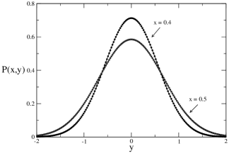
Figure 16: Field probability distribution $p(x,y)$ for the $2+4$ model with $\mu_{2}=2$ and $\mu_{4}=3$ evaluated from the numerical resolution of the Parisi-Sommers-Dupont equations at $x=0.4$ and $x=0.5$. The underlying full curve (barely visible) is the analytic solution given by Eqs. (126), (131).

Appendix B Solution of the Parisi-Sommers-Dupont equations

It is not difficult to write the Parisi-Sommers-Dupont partial differential equations for the 1-FRSB case, cfr. Ref. [CriLeuParRiz04, ]. With obvious notation, the Parisi-Sommers-Dupont functional with the 1-FRSB ansatz reads

$$\beta f_{v} = \beta f+\int_{-\infty}^{+\infty}\,dy\,P(m,y)\Big{[}\phi(m,y)$$ (118)

$$\phantom{xxx}-\frac{1}{2}\frac{y^{2}}{\lambda_{1}-\overline{\lambda}-m\,(\lambda_{1}-\lambda_{0})}\Bigr{]}$$

$$-\int_{0}^{m}\,dx\,\int_{-\infty}^{+\infty}\,dyP(x,y)\Bigl{[}\dot{\phi}(x,y)$$

$$\phantom{xxx}+\frac{1}{2}\dot{\lambda}(x)\left[\phi^{\prime\prime}(x,y)+x\,\phi^{\prime}(x,y)^{2}\Bigr{]}\right]$$

where $\beta f$ is the free energy functional

$$\beta f = -s(\infty)$$ (119)

$$-\frac{1}{2}\bigl{[}g(1)-(1-m)\,g(q_{1})-\int_{0}^{m}\,dx\,g(q(x))\bigr{]}$$

$$+\frac{1}{2}\bigl{[}\overline{\lambda}-(1-m)\,\lambda_{1}q_{1}-\int_{0}^{m}\,dx\,\lambda(x)\,q(x)\bigr{]}$$

$$-\frac{1}{2}\ln\left(\frac{2\pi}{\lambda(1)-\overline{\lambda}}\right)$$

$$-\frac{1}{2m}\ln\left(\frac{\lambda_{1}-\overline{\lambda}}{\lambda_{1}-\overline{\lambda}-m\,(\lambda_{1}-\lambda_{0})}\right)$$

$$-\int_{-\infty}^{+\infty}\,\frac{dy}{\sqrt{2\pi\lambda(0)}}\,\exp\left(-\frac{y^{2}}{2\lambda(0)}\right)\,\phi(0,y)$$

Stationarity of (118) with respect to variations of $P(x,y)$ and $P(m,x)$ yields the Parisi equation (108) with $x$ restricted to the interval $[0,m]$ and initial condition

$$\phi(m,y)=-\frac{1}{2}\frac{y^{2}}{\lambda_{1}-\overline{\lambda}-m\,(\lambda_{1}-\lambda_{0})}$$ (120)

Similarly stationarity with respect to variations of $\phi(x,y)$, $\phi(0,y)$, $q(x)$, $\lambda(x)$ for $0\leq x\leq m$ gives again eqs. (111), (112), (113) and (114), while stationarity with respect to $\overline{\lambda}$ leads back to eq (115) with $\lambda(1)$ replaced by $\lambda_{1}$.

For the 1-FRSB ansatz there are three more equations. The first two follow from stationarity with respect to $q_{1}$, $\lambda_{1}$ and read

$$\lambda_{1}=\Lambda(q_{1})$$ (121)

$$\lambda_{1}-\lambda_{0}=\frac{q_{1}-q_{0}}{(1-q_{1})[1-q_{1}-m\,(q_{1}-q_{0})]}$$ (122)

Finally stationarity with respect to $m$, the discontinuity point in the order parameter function, leads again to equation (55). It is not difficult to recognize in these equations the saddle point equations for $q_{0}$, $q_{1}$ and $m$ derived for the 1-FRSB phase.

For the spherical model the Parisi-Sommers-Dupont equations can be solved analytically. Indeed defining

$$F(x)=\lambda_{1}-\overline{\lambda}-m\,(\lambda_{1}-\lambda_{0})-\int_{x}^{m}\,dx^{\prime}\,x^{\prime}\,\dot{\lambda}(x^{\prime})$$ (123)

it is easy to verify that the solution reads

$$\phi(x,y)=\frac{1}{2}\left[\frac{y^{2}}{F(x)}+\int_{x}^{m}\,dx^{\prime}\,\frac{\dot{\lambda}(x^{\prime})}{F(x^{\prime})}\right]$$ (124)

$$m(x,y)=\frac{y}{F(x)}$$ (125)

and

$$P(x,y)=\frac{1}{\sqrt{2\pi\sigma(x)^{2}}}\,\exp\left(-\frac{y^{2}}{2\sigma(x)^{2}}\right)$$ (126)

where

$$\sigma(x)^{2}=F(x)^{2}\,\int_{0}^{x}\,dx^{\prime}\frac{\dot{\lambda}(x^{\prime})}{F(x^{\prime})^{2}}$$ (127)

Inserting Eqs. (125)-(126) into Eq. (114) one gets

$$q(x)=\int_{0}^{x}\,dx^{\prime}\,\frac{\dot{\lambda}(x^{\prime})}{F(x^{\prime})^{2}}$$ (128)

Taking the derivative of eqs. (123) and (128) with respect to $x$ it is easy to show that

$$\frac{dF}{F^{2}}=x\,dq$$ (129)

which integrated yields the equality $\chi(x)=1/F(x)$. Thus Eq. (128) becomes

$$q(x)=\int_{0}^{x}\,dx^{\prime}\,\dot{\lambda}(x^{\prime})\,\chi(x^{\prime})^{2}$$ (130)

Inverting this relation one gets back Eq. (53). We note that changing the integration variable from $x$ to $q$ in Eq. (128) one can show that $F^{2}(q)=\Sigma(q)$ so that the variance $\sigma(x)^{2}$ of the local field distribution (126) can be written as

$$\sigma(x)^{2}=\Sigma(q(x))\,q(x)$$ (131)

This completes the solution of the Parisi-Sommers-Dupont equations for the spherical $2+p$ spin glass model in the 1-FRSB phase. The FRSB solution can be obtained taking $q_{0}\to q_{1}$ and $m\to 1$.

Appendix C The spherical $s+p$ spin glass model

The spherical $s+p$ spin glass model is the generalization of $2+p$ models in which the two-spin interaction is replaced by a $s$-body spin interaction:

$${\cal H}=\sum_{i_{1}<\ldots<i_{s}}^{1,N}J^{(s)}_{i_{1}\ldots i_{s}}\sigma_{i_{1}}\cdots\sigma_{i_{s}}+\sum_{i_{1}<\ldots<i_{p}}^{1,N}J^{(p)}_{i_{1}\ldots i_{p}}\sigma_{i_{1}}\cdots\sigma_{i_{p}}$$ (132)

In the following we shall assume that $s<p$, even if the Hamiltonian is trivially invariant under the exchange of $s$ and $p$.

The study of the $s+p$ model follows closely that of the $2+p$ with the replacement of $g(x)$ by [see Eq. (12)]

$$g(x)=\frac{\mu_{s}}{s}x^{s}+\frac{\mu_{p}}{p}x^{p}.$$ (133)

As it happens for the $2+p$ models the RS solution with $q\not=0$ is unstable, however, at difference with these, the RS solution with $q=0$ is stable everywhere in the $(\mu_{p},\mu_{s})$ plane since for $q=0$ the relevant eigenvalue $\Lambda_{1}$, eq.(21), is identically equal to one for any $s>2$.

For $\mu_{p}$ and/or $\mu_{2}$ large enough a thermodynamically more favorable 1RSB solution appears. This solution has $q_{0}=0$ and $q_{1}$ given by the saddle point equation (29) [with $q_{0}=0$]. For the static solution the value of $m$ is fixed by Eq. (30), or equivalently by Eq. (33), which follows from stationarity of the free energy functional with respect to variations of $m$. These equations can be solved for any $s$ and $p$ with the help of the CS $z$-function and one obtains the parametric equations of the static $m$-lines:

$$\mu_{p} = \frac{p}{(p-s)}\,\frac{(1-y+m\,y)^{p}}{m^{2}y(1-y)^{p-2}}\,\frac{[2-s\,z(y)]}{2}$$ (134)

$$\mu_{s} = \frac{s}{(p-s)}\,\frac{(1-y+m\,y)^{s}}{m^{2}y(1-y)^{s-2}}\,\frac{[p\,z(y)-2]}{2}$$ (135)

where $y=(1-q_{1})/(1-q_{1}+m\,q_{1})$. Notice that, as expected, the expressions are symmetric under the exchange of $s$ and $p$.

The 1RSB solution never becomes unstable since for $s>2$ the eigenvalue $\Lambda_{0}^{(3)}$, Eq. (31), evaluated at $q_{0}=0$ is always positive, and the eigenvalue $\Lambda_{1}^{(1)}$, Eq. (32), remains positive for any $\mu_{p}\geq 0$.

As a consequence the limit on $y$ are given by the conditions

$$\mu_{p}=0\ \Rightarrow \ z(y_{\mu_{p}})=\frac{2}{s}$$ (136)

$$\mu_{s}=0\ \Rightarrow \ z(y_{\mu_{s}})=\frac{2}{p}$$ (137)

The CS $z$-function is an increasing function of $y$ therefore if $s<p$ then $y_{\mu_{p}}<y_{\mu_{s}}$. For $s=3$ and $p=4$ we have

$$y_{\mu_{4}}=0.195478...,\quad y_{\mu_{3}}=0.354993...$$ (138)

To find the dynamic transition line between the 1RSB and the RS phase equation (33) must be replaced by the marginal condition (91). Using $q_{1}$ as the independent variable it is easy to derive the parametric equations for the dynamic $m$-lines:

$$\mu_{p} = \frac{1}{(p-s)}\,\frac{(s-2+m)\,q_{1}-(s-2)}{q_{1}^{p-2}\,(1-q_{1})^{2}\,(1-q_{1}+m\,q_{1})}$$ (139)

$$\mu_{s} = \frac{1}{(p-s)}\,\frac{(p-2)-(p-2+m)\,q_{1}}{q_{1}^{s-2}\,(1-q_{1})^{2}\,(1-q_{1}+m\,q_{1})}$$ (140)

The range of $q_{1}$ is fixed by the requirement that both $\mu_{p}$ and $\mu_{s}$ be non-negative. This yields the boundary values

$$\mu_{p}=0\ \Rightarrow \ q_{1}=\frac{s-2}{s-2+m}$$ (141)

$$\mu_{s}=0\ \Rightarrow \ q_{1}=\frac{p-2}{p-2+m}$$ (142)

In Figure 17 we show the phase diagram for the $s+p$ model with $s>2$ and $p>s$. In the figure $s=3$ and $p=4$, however any choice of $s>2$ and $p>s$ leads to a qualitatively similar phase diagram.

Figure 17: The phase diagram of the $3+4$ model in the $(\mu_{3},\mu_{4})$ plane. The thick dashed lines are the $m$-line with $m=1$, i.e. represent the discontinuous transition between the RS and the 1RSB phases.

Appendix D The RSB Solutions

In this Appendix we show that the spherical $2+p$ spin glass model admits only solutions of 1RSB, FRSB or 1-FRSB type. The procedure is the same as that of Appendix 2 of Ref. [CriSom92, ].

We start from the free energy functional for the $R$-RSB ansatz [see Eq. (46)]

$$\frac{2}{n}\,G[{\bm{q}}] = \int_{0}^{1}dq~{}x(q)\,\Lambda(q)$$ (143)

$$+\int_{0}^{q_{R}}\frac{dq}{\int_{q}^{1}dq^{\prime}\,x(q^{\prime})}+\ln\left(1-q_{R}\right)$$

where

$$x(q)=p_{0}+\sum_{r=0}^{R}(p_{r+1}-p_{r})\,\theta(q-q_{r}).$$ (144)

The saddle point equations are obtained by varying the above functional with respect to $x(q)$:

$$\frac{2}{n}\,\delta G[{\bm{q}}]=\int_{0}^{1}\,dq\,F(q)\,\delta x(q)$$ (145)

where

$$F(q)=\Lambda(q)-\int_{0}^{q}\frac{dq^{\prime}}{\left[\int_{q^{\prime}}^{1}dq^{\prime\prime}\,x(q^{\prime\prime})\right]^{2}}$$ (146)

and

$$\delta x(q) = \sum_{r=0}^{R}\,(\delta p_{r+1}-\delta p_{r})\,\theta(q-q_{r})$$ (147)

$$-\sum_{r=0}^{R}\,(p_{r+1}-p_{r})\,\delta(q-q_{r})\,\delta q_{r}$$

By requiring stationarity of $G[{\bm{q}}]$ with respect to the $q_{r}$ and the $p_{r}$ one gets, respectively

$$F(q_{r})=0,\qquad r=0,\ldots,R$$ (148)

$$\int_{q_{r-1}}^{q_{r}}\,dq\,F(q)=0,\qquad r=1,\ldots,R$$ (149)

The function $F(q)$ is continuous, thus Eq. (149) implies that between any two successive $q_{r}$ there must be at least two extrema of $F(q)$. If we denote these by $q^{*}$, then the extremal condition $F^{\prime}(q^{*})=0$ implies that

$$\int_{q^{*}}^{1}\,dq\,x(q)=\frac{1}{\sqrt{\Sigma(q^{*})}}$$ (150)

The left hand side of this equation is a concave function, i.e. with a negative second derivative, since $x(q)$ is not decreasing with $q$. For the $2+p$ model $\Sigma(q)=\mu_{2}+\mu_{p}(p-1)q^{p-2}$ so that the right hand side is concave for small $q$, provided $p>3$, and convex for large $q$, see Figure 18. For $p=3$ the right hand side is convex.

As a consequence Eq. (150) admits at most two solutions and hence only one step of replica symmetry breaking is possible.

Figure 18: Typical behavior of $1/\sqrt{\Sigma(q)}$ as function of $q$ for $p>3$.

Moreover it must be $q_{0}=0$. Indeed, from Eq. (148) and from the fact that in absence of external field $F(0)=0$ it follows that

$$F(0)=F(q_{0})=F(q_{1})=0$$ (151)

which would imply the presence of at least three extrema, which is not possible.

Up to this point the conclusions do not differ much from those found for the $p$-spin model. Here however the presence of a concave part in the right hand side of Eq. (150) for $p>3$ makes possible different solutions.

Equations (148) and (149) can be solved by a continuous replica symmetry breaking solution with $F(q)=0$ in a given range of $q$ since in this case both equations would be identically valid. For this solution Eq. (150) must also be identically valid and this can only be true for $0\leq q\leq q_{0}$, where $q_{0}$ is the value of $q$ for which $1/\sqrt{\Sigma(q)}$ changes concavity, where both sides of the equation are concave function of $q$. Indeed if Eq. (150) were valid also for values of $q$ where the right hand side is convex this would imply that $x(q)$ is a decreasing function of $q$, which is not possible since $dx(q)/dq$ is the probability density of the overlaps. For the same reason for $p=3$ a continuous replica symmetry breaking solution is not allowed since in this case the right hand side of Eq. (150) is purely convex. The same applies to the $s+p$ models with $s>2$, so that also these models admits only a 1RSB phase.

The possibility of a continuous replica symmetry breaking solution for $q\leq q_{0}$ does not rule out the presence of discrete replica breakings with $q_{r}>q_{0}$. These additional discrete breakings must satisfy eqs. (148) and (149). Therefore since the right hand side of Eq. (150) is convex for $q>q_{0}$ arguments similar to those which leaded to the conclusion that for the $2+3$ model only 1RSB solutions are possible show that at most only one more discrete break with $q_{1}>q_{0}$ is possible.

No other possible non trivial solutions exist for the spherical $2+p$ spin glass model so we conclude that the model admits only solutions of 1RSB, 1-FRSB or FRSB type.

References

- (1) T.R. Kirkpatrick and D. Thirumalai, Phys. Rev. B, 36, 5388 (1987).
- (2) A. Crisanti and H-.J. Sommers, Z. Phys. B 87, 341 (1992).
- (3) J. P. Bouchaud, L. F. Cugliandolo, J. Kurchan and M. Mézard in Spin glasses and random fields A. P. Young ed. (World Scientific, Singapore, 1997).
- (4) Th. M. Nieuwenhuizen, Phys. Rev. Lett. 74, 4289 (1995).
- (5) A.J. Bray and M.A. Moore, Phys. Rev Lett. 41, 1068 (1978).
- (6) E. Pytte and J. Rudnick, Phys. Rev. B 19, 3603 (1979).
- (7) S. Ciuchi and A. Crisanti, Europhys. Lett 49, 754 (2000).
- (8) W. Götze and L. Sjörgen, J. Phys. Cond. Matt. 1, 4203 (1989).
- (9) A. Crisanti and L. Leuzzi, Phys. Rev. Lett. 93, 217203 (2004).
- (10) O.B. Tsiok, V.V. Brazhkin, A.G. Lyapin and L.G. Khvostantsev, Phys. Rev. Lett. 80, 999 (1998).
- (11) L. Huang and J. Kieffer, Phys. Rev. B, 69, 224203 (2004).
- (12) S. K. Deb, M. Wilding, M. Somayazulu and P.F. McMillan, Nature, 414, 528 (2001).
- (13) P.H. Poole et al., Nature 360, 324 (1992); P.H. Poole et al., Phys. Rev. E 48, 4605 (1993).
- (14) K. Dawson et. al., Phys. Rev. E 63, 011401 (2001).
- (15) E. Zaccarelli, G. Foffi, K.A. Dawson, F. Sciortino and P. Tartaglia, Phys. Rev. E, 63, 031501 (2001).
- (16) F. Sciortino, Nature 1, 145 (2002).
- (17) S.-H.Chen, W.R. Chen, F. Mallamace, Science 300, 619 (2003).
- (18) T. Eckert and E. Bartsch, Phys. Rev. Lett. 89, 125701 (2002).
- (19) K.N. Pham, Science 296, 104 (2002).
- (20) A. Caiazzo, A. Coniglio and M. Nicodemi, Phys. Rev. Lett. 93, 215701 (2004).
- (21) T.R. Kirkpatrick and P.G. Wolynes, Phys. Rev. B 36, 8552 (1987).
- (22) A. Crisanti, H. Horner and H.-J. Sommers Z. Phys. B 92, 257 (1993).
- (23) A. Crisanti and Th. M. Nieuwenhuizen, Journal de Physique I France 6, 56 (1996).
- (24) S.F. Edwards and P.W. Anderson, J. Phys. F 5, 965 (1975).
- (25) G. Parisi, J. Phys. A 13, L115, 1101 and 1887 (1980).
- (26) A. Annibale, G. Gualdi and A. Cavagna, J. Phys. A 37, 11311 (2004).
- (27) S.K. Ma, Modern Theory of Critical Phenomena, Frontiers in Physics Lecture Note Series, 46, (Benjamin/Cummings Publishing, 1976)
- (28) M. Mezárd, G. Parisi and M.Virasoro, Spin Glass Theory and Beyond (World Scientific, Singapore, 1987).
- (29) K.H. Fischer and J.A. Hertz, Spin Glasses (Cambridge University Press, Cambridge, England, 1991)
- (30) D. Sherrington, and S. Kirkpatrick, Phys. Rev. Lett. 35 (1975) 1792.
- (31) The replica trick uses the identity and hence should be known for a continuous set of values of and not just for integers. Consequence of this is that the limit is not the analytic continuation of down to .
- (32) F. Guerra and F.L. Toninelli, Commun. Math. Phys. 230, 71 (2002).
- (33) M. Talagrand, C.R. Acad.Sci. Paris, Ser. I 337, 111 (2003); Annals of Mathematics, to appear.
- (34) The calculation of the eigenvalues of the quadratic form (17) for 1RSB solution of the model does not differ much from that of the spherical -spin model. As a consequence to help the reader interested into the details of the derivation we shall use for the eigenvalues the same notation as Ref. [CriSom92, ].
- (35) J.R.L. de Almeida, D.J. Thouless, J. Phys. A 11, 983 (1978).
- (36) and are two of the eigenvalues of the overlap matrix in the 1RSB ansatz denoted respectively and in Ref. [CriSom92, ].
- (37) For finite the saddle point calculation requires that be maximal at the stationary point. However the dimension of the -space becomes negative for so that should be minimized in the limit . Consistently the free energy functional is maximized for .
- (38) The lowest value of the order parameter matrix is the minimum possible overlap between replicas. It is always zero in absence of an external field.
- (39) A. Crisanti, (1986) unpublished
- (40) C. De Dominicis and D. M. Carlucci, C. R. Acar. Sci. Paris 323, 263 (1996); C. De Dominicis, D. M. Carlucci and T. Temesvári, J. Phys. I France 7, 105 (1997).
- (41) G. Parisi, Phys. Rev. Lett. 43, 1754 (1979).
- (42) The most general form of the order parameter function in the 1RSB phase is . However, in absence of external fields, .
- (43) To maintain the notation for the overlap associated to the 1RSB part of the order parameter function we use the notation for the largest value of the continuous part of the order parameter function. This notation should not be confusing since .
- (44) A. Crisanti, L. Leuzzi, G. Parisi, J. Phys. A 35 481 (2002).
- (45) C. De Dominicis and I. Kondor, Phys. Rev. B 27, 606 (1983); I. Kondor and C. De Dominicis, J. Phys. A 16, L73 (1983).
- (46) A. Crisanti and T. Rizzo, Phys. Rev. E 65, 046137 (2002).
- (47) In the expansion given in Ref.[CriLeu04, ] the exponent of the third term is erroneously given as .
- (48) A. Crisanti and H-.J. Sommers J. Phys. I (France) 5, 805 (1995).
- (49) A. Crisanti L. Leuzzi, T. Rizzo, Eur. Phys. J. B 36, 129 (2003).
- (50) T. Plefka, J. Phys. A. 15, 1971 (1982); Europhys. Lett. 58, 892 (2002).
- (51) A. Crisanti L. Leuzzi, in preparation.
- (52) H. Sompolinsky, Phys. Rev. Lett. 47, 935 (1981).
- (53) C. de Dominicis et al., J. Phys. A: Math. Gen. 15, L47 (1982).
- (54) S. Franz, M. Mezárd, G. Parisi, L. Peliti, Phys. Rev. Lett. 81, 1758 (1998); S. Franz, M. Mezárd, G. Parisi, L. Peliti, J. Stat. Phys. 97, 459 (1999).
- (55) Such phase can be built ad hoc also in the case of discrete variables but it turns out to be always unstable. CriLeuParRiz04
- (56) H-.J. Sommers and W. Dupont, J. Phys. C 17, 5785 (1984)
- (57) A. Crisanti, L. Leuzzi, G. Parisi and T. Rizzo, Phys. Rev. B 70, 064423 (2004).