Faraday rotation in photoexcited semiconductors:
an excitonic many-body effect

Abstract

This letter assigns the Faraday rotation in photoexcited semiconductors to “Pauli interactions”, i. e., carrier exchanges, between the real excitons present in the sample and the virtual excitons coupled to the $\sigma_{\pm}$ parts of a linearly polarized light. While direct Coulomb interactions scatter bright excitons into bright excitons, whatever their spins are, Pauli interactions do it for bright excitons with same spin only. This makes these Pauli interactions entirely responsible for the refractive index difference, which comes from processes in which the virtual exciton which is created and the one which recombines are formed with different carriers. To write this difference in terms of photon detuning and exciton density, we use our new many-body theory for interacting excitons. Its multiarm “Shiva” diagrams for $N$-body exchanges make transparent the physics involved in the various terms. This work also shows the interesting link which exists between Faraday rotation and the exciton optical Stark effect.

PACS.71.35.-y – Excitons and related phenomena.

It is known since a long time that the polarization plane of a linear light rotates when passing through an optically active medium. This effect, known as Faraday rotation, is usually explained rather phenomenologically, by saying that, due to a dissymmetry in the sample — which can preexist or be induced — the $\sigma_{\pm}$ components of the light have different refractive indices $n_{\pm}$, the rotation of the polarization plane being proportional to $(n_{+}-n_{-})$. From a microscopic point of view, this difference has to come from difference in the interactions of the sample with the virtual excitations coupled to the unabsorbed $\sigma_{\pm}$ photons. Faraday rotation is thus a powerful tool to study not only these interactions, but also the excited state relaxations, in particular, spin relaxation crucial for spintronics [1-6]. In order to fully control these studies, a precise microscopic understanding of this rotation is however highly desirable.

In the case of semiconductors, the matter excitations are the excitons. With respect to their possible interactions, doped and photoexcited samples are very different. Indeed, due to Pauli exclusion, the free carriers of a doped sample have different energies; this makes their possible interactions with the virtual excitons coupled to photons rather tricky. Using experimental results on Faraday rotation and circular dichroism, we have recently suggested [7] that these carriers do not form trions, as commonly said, but an intrinsically wide many-body object, singular at threshold. Photoexcited samples are, in this respect, simpler because the excitons they contain have an energy which is essentially constant for very heavy holes. However, even in this case, a fully microscopic theory of Faraday rotation has not been easy to produce because interactions between excitons are difficult to handle properly due to the exciton composite nature — which is here crucial.

Our new many-body theory for composite bosons [8] now provides a quite efficient tool to face such a problem. The diagrammatic representation we have recently proposed [9], with its multiarm “Shiva” diagrams [10] to visualize $N$-body exchanges, allows a keen understanding of the physics involved in the various terms.

1 Microscopic approach

A microscopic description of Faraday rotation goes through the determination of the linear response function $S_{\sigma}$ of the material to a probe beam with circular polarization $\sigma=\pm 1$. This response function, for a matter state $|\psi\rangle$, reads [11]

$$S_{\sigma}=\langle\psi|U_{\sigma}\,\frac{1}{\omega+\mathcal{E}-H+iO_{+}}\,U_{\sigma}^{\dagger}|\psi\rangle\ ,$$ (1)

where $\omega$ is the photon energy, $\mathcal{E}$ the state $|\psi\rangle$ energy and $H$ the matter Hamiltonian. For semiconductors, the matter coupling to $\sigma$ photons can be written as $U_{\sigma}^{\dagger}=\sum_{I}\delta_{S_{i},\sigma}\mu_{i}^{\ast}B_{I}^{\dagger}$, where $B_{I}^{\dagger}$ creates an exciton $I=(i,S_{i})$ with spin $S_{i}$, in a state $i=(\nu_{i},\mathbf{Q}_{i})$, while $|\mu_{i}|$ is the $i$ exciton Rabi energy [12]. The refractive index difference is related to this response function through $n_{+}-n_{-}\simeq\mathrm{Re}(S_{+1}-S_{-1})/\mathcal{E}_{p}$, where $\mathcal{E}_{p}$ is an energy like constant [13].

2 Physical origin

Let us concentrate on quantum wells previously excited by $\sigma_{+}$ pump photons tuned on the ground state exciton. Before spin relaxation, this sample essentially contains $N$ ground state excitons $(S=1)$, made of (3/2) hole and (-1/2) electron, the corresponding matter state being [14]

$$|\psi\rangle\simeq[N!F_{N}]^{-1/2}\,B_{O}^{{\dagger}N}|v\rangle\ ,$$ (2)

where $B_{O}^{\dagger}$ creates an exciton $O=(\nu_{o},\mathbf{Q}_{o},S_{o}=1)$ in the $\nu_{o}$ relative motion ground state, the exciton momentum $\mathbf{Q}_{o}$ being essentially the pump photon momentum. $N!F_{N}=\langle v|B_{O}^{N}B_{O}^{{\dagger}N}|v\rangle$ is a normalization factor which differs from $N!$ due to the exciton composite nature [15].

In $S_{\sigma}$, the operator $U_{\sigma}^{\dagger}$ adds a virtual exciton $I$ to these $N$ excitons $O$, while $U_{\sigma}$ destroys a virtual exciton $I^{\prime}$, a priori different from $I$: As photons interact with a semiconductor through the virtual excitons to which they are coupled, the response function comes from the interactions of $I$ with the excitons present in the sample. The exciton $I^{\prime}$ which recombines thus results from all the interactions between $I$ and $|\psi\rangle$ which leave $|\psi\rangle$ unchanged.

If we now consider spins, the exciton $I^{\prime}$ restoring a $\sigma_{\pm}$ photon must have a $(\pm 3/2)$ hole and a $(\mp 1/2)$ electron. As fermions are indistinguishable, these carriers can be either the ones of $I$ or any other similar carriers. The physical reason for $S_{+1}\neq S_{-1}$ then becomes transparent: If the sample contains $N$ holes $(3/2)$ and $N$ electrons $(-1/2)$, the virtual exciton $I^{\prime}$ in $S_{-1}$, which regenerates a $\sigma_{-}$ photon, can only be made of the $(-3/2,1/2)$ carriers of $I$. On the opposite, $I^{\prime}$ in $S_{+1}$, which regenerates a $\sigma_{+}$ photon, can be made either of the $I$ carriers or of any of the $N$ holes $(3/2)$ and the $N$ electrons $(-1/2)$ present in the sample. The processes in which $I^{\prime}$ is made of carriers different from $I$ — one of the two carriers being possibly the same — are thus the ones producing $S_{+1}$ different from $S_{-1}$.

To go further and identify these processes precisely, we make use of the two elementary scatterings of our many-body theory for composite excitons, namely the (energy-like) direct Coulomb scatterings, in which the “in” and “out” excitons keep their carriers, and the (dimensionless) Pauli scatterings in which the excitons exchange their carriers without Coulomb.

Due to spin conservation, Pauli scatterings scatter bright excitons into bright excitons if they have the same spin only, while (direct) Coulomb scatterings do it whatever their relative spins are. Consequently, as the exciton $I^{\prime}$ has to be bright to restore a photon, carrier exchanges through Pauli scatterings between $I$ and $O$ can produce a bright $I^{\prime}$ if $I$ and $O$ have same spin only, i. e., if the pump and the probe have the same circular polarization.

3 Dependences in detuning and exciton density

Let us now feel the physics which controls the dependence of $(S_{+1}-S_{-1})$ on the two parameters of the problem, namely the probe photon detuning $\Omega=E_{g}-\omega$, and the density $N/L^{D}$ of excitons in a sample of size $L$ in $D$ dimension. These parameters can be associated to the dimensionless quantities

$$\gamma=R_{X}/\Omega\ ,\hskip 56.9055pt\eta=N(a_{X}/L)^{D}\ ,$$ (3)

where $(R_{X},a_{X})$ are the 3D exciton Rydberg and Bohr radius.

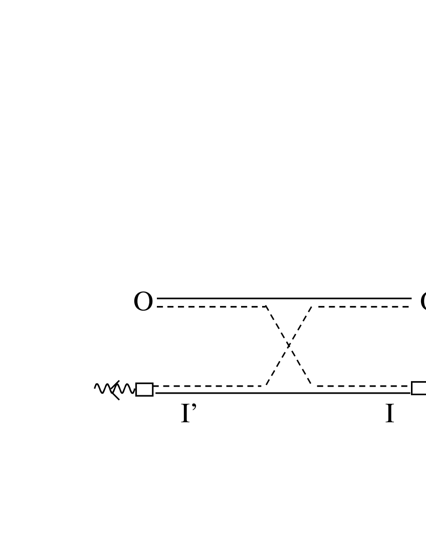
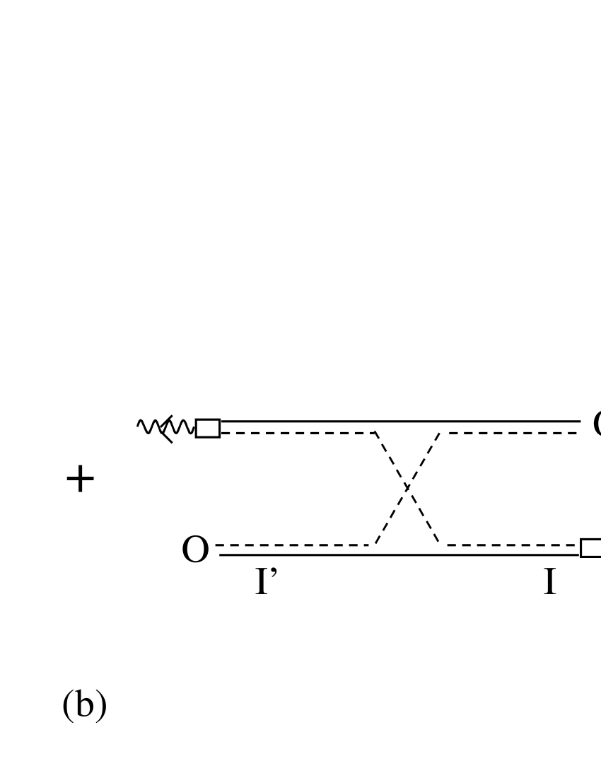
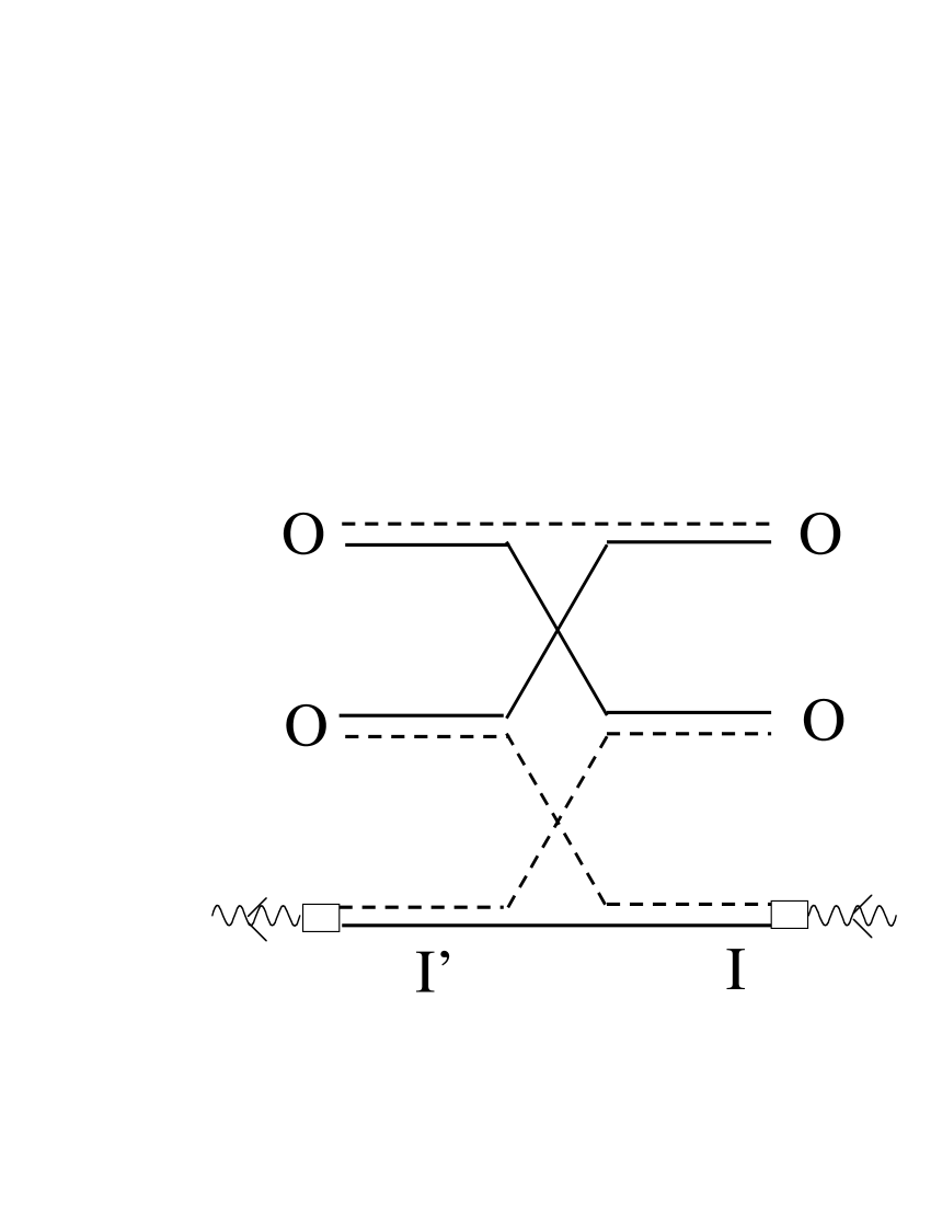
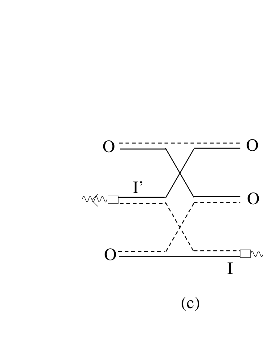
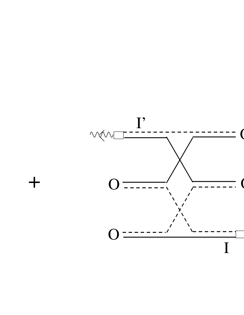
Figure 1: (a) the “box” a priori contains any number of Pauli (exchange without Coulomb) and Coulomb (without exchange) scatterings between the virtual exciton $I$ coupled to the $\sigma$ photon and the $N$ excitons $O$ present in the sample; the only requirement is to restore the $N$ excitons $O$. Electrons are represented by solid lines and holes by dashed lines, the double solid-dashed lines representing the excitons. (b,c) Multiarm “Shiva” diagrams for Pauli scatterings between $I$ and one or two excitons $O$. Faraday rotation is due to processes in which the virtual excitons $I$ and $I^{\prime}$ have zero or one common carrier.

The response function $S_{\sigma}$ defined in eq.(1) can be represented by the diagram of fig.1a. In the “box”, any Pauli or Coulomb interaction between $I$ and the $N$ excitons $O$ can take place, provided that the electron and hole spins of $I^{\prime}$ are the ones of $I$, to restore the $\sigma$ photon.

The $\gamma$ dependence of $S_{\sigma}$ can be understood through dimensional arguments. In view of eq.(1), $S_{\sigma}$ a priori contains two couplings, $U_{\sigma}$ and $U_{\sigma}^{\dagger}$, i. e., two Rabi energies, and one energy denominator, of the order of the detuning. If the excitons in the “box” interact via Coulomb scatterings, other energy denominators, i. e., detunings, must appear to compensate the Coulomb scattering dimension, while this is unnecessary if they interact through the dimensionless Pauli scatterings. Consequently, the $\gamma$ leading term comes from processes with zero Coulomb interaction.

We now turn to the density dependence. Processes in which the exciton $I$ interacts with one exciton $O$, must appear with a factor $N$, as there is $N$ ways to choose this exciton among the $N$ excitons $O$. These processes produce the $\eta$ linear terms of $S_{\sigma}$. In the same way, processes in which $I$ interacts with two excitons $O$ produce the $\eta^{2}$ terms, as there are $N(N-1)$ ways to choose two excitons among $N$. And so on …

Let us now visualize these various processes, using our multiarm “Shiva” diagrams for $N$-body exchanges:

(i) The $\gamma$ leading term, linear in $\eta$, is due to Pauli scatterings between $I$ and $p=1$ exciton $O$ (see fig.1b). In these processes, the excitons $I^{\prime}$ and $I$ have one common carrier. Obviously, the pump and the probe must have the same circular polarization for these diagrams to exist.

(ii) The $\gamma$ leading term, quadratic in $\eta$, is due to Pauli scatterings between $I$ and $p=2$ excitons $O$ (see fig.1c). In the two first diagrams, $I^{\prime}$ and $I$ have one common carrier, while in the last diagram, their two carriers are different. And so on…for the $\eta^{p}$ term.

(iii) The next order term in $\gamma$ comes from processes with one Coulomb interaction between $I$ and the excitons $O$. In the $\eta$ term, only one of these $O$ excitons enters. It is constructed on the diagrams of fig.1b, with the Coulomb scattering between any two exciton lines. The $\eta^{2}$ term is constructed in a similar way on the diagrams of fig.1c. And so on …

We could think that processes with one Coulomb scattering, i. e., two detuning denominators, should behave as $\gamma^{2}$. This is more subtle. The virtual excitons coupled to probe photons are not necessarily ground state excitons, for no energy conservation is required for virtual processes. It turns out that the exciton extended states give a singular contribution to $S_{\sigma}$ which, at large detuning, transforms the naïve $\gamma^{2}$ dependence into $\gamma^{3/2}$. A way to understand it, is to say that counting processes with 0, 1, 2…Coulomb interactions amounts to perform an expansion in $e^{2}$, proportional to $\gamma^{1/2}$.

By calculating precisely all these contributions, we eventually find that the expansion of the refractive index difference in terms of $\gamma$ and $\eta$ reads, for a 2D structure,

$$n_{+}-n_{-}\simeq f\,\left[\gamma\{2\eta-(4\pi/5)\eta^{2}+O(\eta^{3})\}+\gamma^{3/2}\{3\pi\eta+O(\eta^{2})\}+O(\gamma^{2})\right]\ ,$$ (4)

where $f=|\mu|^{2}/\mathcal{E}^{\prime}_{p}R_{X}$ is a dimensionless constant, with $\mathcal{E}^{\prime}_{p}=\mathcal{E}_{p}(a_{X}/L)^{D}$ and $|\mu|$ being energies free of sample size (see [12] and [13]).

4 Main steps of the theory

This understanding may appear as wishful thinkings. It actually follows from our many-body theory for composite excitons.

(i) The Coulomb expansion of $S_{\sigma}$, is obtained by passing the $B_{I}^{\dagger}$’s of $U_{\sigma}^{\dagger}$ over the Hamiltonian, through [8]

$$(a-H)^{-1}B_{I}^{\dagger}=[B_{I}^{\dagger}+(a-H)^{-1}V_{I}^{\dagger}](a-H-E_{i})^{-1}\ ,$$ (5)

which follows from $V_{I}^{\dagger}=[H,B_{I}^{\dagger}]-E_{i}B_{I}^{\dagger}$, where $E_{i}$ is the $I$ exciton energy.

This leads to split $S_{\sigma}$ as $S_{\sigma}^{(0)}+S_{\sigma}^{(1)}+S_{\sigma}^{\mathrm{(corr)}}$, where $S_{\sigma}^{(0,1)}$ are zero and first order in the “creation Coulomb potential” $V_{I}^{\dagger}$, while $S_{\sigma}^{\mathrm{(corr)}}$ contains all higher order terms:

$$S_{\sigma}^{(0)}=\sum_{I^{\prime},I}\frac{\delta_{S_{i^{\prime}},\sigma}\,\delta_{S_{i},\sigma}}{2\Delta_{i}}\,\left[\mu_{i^{\prime}}\mu_{i}^{\ast}\,\langle\psi|B_{I^{\prime}}\,B_{I}^{\dagger}|\psi\rangle\,+c.c.\right]\ ,$$ (6)

$$S_{\sigma}^{(1)}=\sum_{I^{\prime},I}\frac{\delta_{S_{i^{\prime}},\sigma}\,\delta_{S_{i},\sigma}}{2\Delta_{i^{\prime}}\Delta_{i}}\,\left[\mu_{i^{\prime}}\mu_{i}^{\ast}\,\langle\psi|B_{I^{\prime}}V_{I}^{\dagger}|\psi\rangle\,+c.c.\right]\ ,$$ (7)

where $\Delta_{i}=(-\Omega_{i}+i0_{+})$, with $\Omega_{i}=E_{i}-\omega$ being the $I$ exciton detuning.

(ii) In $S_{\sigma}^{(0)}$, appear the scalar products of $(N+1)$ excitons. They are calculated using

$$\left[B_{M},B_{O}^{{\dagger}N}\right]=N\,B_{O}^{{\dagger}N-1}\,(\delta_{M,O}-D_{MO})-N(N-1)\sum_{P}\Lambda_{h}\left({}_{M}^{P}\ {}_{O}^{O}\right)\,B_{P}^{\dagger}B_{O}^{{\dagger}N-2}\ ,$$ (8)

which is a generalization for $N>1$, of the equation which defines the “deviation-from-boson” operator $D_{MO}$ [8]. This operator is then eliminated through

$$\left[D_{MI},B_{J}^{\dagger}\right]=\sum_{P}\left[\Lambda_{h}\left({}_{M}^{P}\ {}_{I}^{J}\right)+\Lambda_{h}\left({}_{P}^{M}\ {}_{I}^{J}\right)\right]\,B_{P}^{\dagger}\ ,$$ (9)

where the Pauli scattering $\Lambda_{h}\left({}_{M}^{P}\ {}_{I}^{J}\right)$ corresponds to a hole exchange between $I$ and $J$.

For excitons $(I^{\prime},I)$ coupled to the probe and excitons $O$ created by a pump with different wavelength, i. e., $\mathbf{Q}_{i^{\prime}}=\mathbf{Q}_{i}\neq\mathbf{Q}_{o}$, the scalar products of interest [16] in $S_{\sigma}^{(0)}$ reduce to

$$\langle v|B_{O}^{N}B_{I^{\prime}}B_{I}^{\dagger}B_{O}^{{\dagger}N}|v\rangle=\delta_{S_{i^{\prime}},S_{i}}\left\{A_{N}\delta_{i^{\prime},i}+\delta_{S_{i},S_{o}}\left[-A_{N-1}N^{2}\,I_{2}^{(0)}(i^{\prime},i)\right.\right.$$

$$\left.\left.+A_{N-2}N^{2}(N-1)^{2}\,I_{3}^{(0)}(i^{\prime},i)+\cdots\right]\right\}\ ,$$ (10)

with $A_{N}=N!F_{N}$. The processes corresponding to $I_{2,3}^{(0)}$ are the carrier exchanges of figs.1b,c. For a $\sigma_{+}$ pump, this leads to $S_{-1}^{(0)}=\sum_{i}|\mu_{i}|^{2}/\Delta_{i}$, while

$$S_{+1}^{(0)}-S_{-1}^{(0)}=\sum_{i^{\prime}i}\frac{1}{2\Delta_{i}}\,\left\{\mu_{i^{\prime}}\mu_{i}^{\ast}\left[-N\frac{F_{N-1}}{F_{N}}\,I_{2}^{(0)}(i^{\prime},i)+N(N-1)\frac{F_{N-2}}{F_{N}}\,I_{3}^{(0)}(i^{\prime},i)+\cdots\right]\ +c.c.\right\}\ .$$ (11)

(iii) To calculate the first order term in Coulomb scatterings $S_{\sigma}^{(1)}$, we use

$$\langle v|B_{O}^{N}B_{I^{\prime}}V_{I}^{\dagger}B_{O}^{{\dagger}N}|v\rangle=N\sum_{JK}\Xi\left({}_{J}^{K}\ {}_{I}^{O}\right)\langle v|B_{O}^{N}B_{I^{\prime}}B_{J}^{\dagger}B_{K}^{\dagger}B_{O}^{{\dagger}N-1}|v\rangle\ ,$$ (12)

which results from the generalization for $N>1$ excitons of the equation which defines the (direct) Coulomb scatterings, namely

$$\left[V_{I}^{\dagger},B_{O}^{{\dagger}N}\right]=N\,\sum_{JK}\Xi\left({}_{J}^{K}\ {}_{I}^{O}\right)\,B_{J}^{\dagger}B_{K}^{\dagger}\,B_{O}^{{\dagger}N-1}\ .$$ (13)

The remaining scalar products of $(N+1)$ excitons are then calculated in the same way as for $S_{\sigma}^{(0)}$. We end with

$$S_{+1}^{(1)}-S_{-1}^{(1)}=\sum_{i^{\prime}i}\frac{1}{2\Delta_{i^{\prime}}\Delta_{i}}\,\left\{\mu_{i^{\prime}}\mu_{i}^{\ast}\left[N\frac{F_{N-1}}{F_{N}}\,I_{2}^{(1)}(i^{\prime},i)-N(N-1)\frac{F_{N-2}}{F_{N}}\,I_{3}^{(1)}(i^{\prime},i)+\cdots\right]\ +c.c.\right\}\ .$$ (14)

The processes of $I_{2}^{(1)}(i^{\prime},i)$ are the ones of $I_{2}^{(0)}(i^{\prime},i)$ with the Coulomb scattering before the carrier exchange, while in the ones of its complex conjugate, it is after the exchange.

(iv) By using $F_{N-p}/F_{N}\simeq(F_{N-1}/F_{N})^{p}$ for $p\ll N$, with $F_{N-1}/F_{N}\simeq 1+4\pi\eta/5+O(\eta^{2})$ in 2D [15], eqs.(11,14) lead to

$$S_{+1}-S_{-1}\simeq\left(L/a_{X}\right)^{D}|\mu|^{2}\left\{\eta\,a(\omega)+\eta^{2}\left[\frac{4\pi}{5}a(\omega)-b(\omega)\right]+O(\eta^{3})\right\}\ ,$$ (15)

where $a(\omega)$ precisely reads

$$a(\omega)=\frac{1}{2}\sum_{i^{\prime}i}\frac{\mu_{i^{\prime}}\mu_{i}^{\ast}}{|\mu|^{2}}\left(\frac{I_{2}^{(0)}(i^{\prime},i)}{\Omega_{i}}+\frac{I_{2}^{(1)}(i^{\prime},i)}{\Omega_{i^{\prime}}\Omega_{i}}+\cdots\right)\ +c.c.\ =a^{(0)}(\omega)+a^{(1)}\omega)+\cdots\ ,$$ (16)

with $\left(I_{2}^{(0)}(i^{\prime},i),\,I_{2}^{(1)}(i^{\prime},i)\right)$ replaced by $(L/a_{X})^{D}\left(I_{3}^{(0)}(i^{\prime},i),\,I_{3}^{(1)}(i^{\prime},i)\right)$ to get $b(\omega)$. By performing the sums over $i$ in $a(\omega)$ through closure relations, we find

$$a^{(0)}(\omega)=\sum_{\mathbf{k}}G_{\mathbf{k}}(\omega)|\langle\mathbf{k}|\nu_{o}\rangle|^{2}\ +c.c.\ ,$$ (17)

$$a^{(1)}(\omega)=\sum_{\mathbf{k},\mathbf{k}^{\prime}}V_{\mathbf{k}^{\prime}-\mathbf{k}}\langle\mathbf{k}|\nu_{o}\rangle\,\left[\langle\nu_{o}|\mathbf{k}\rangle-\langle\nu_{o}|\mathbf{k}^{\prime}\rangle\right]G_{\mathbf{k}^{\prime}}(\omega)\left[G_{\mathbf{k}}^{\ast}(\omega)-G_{\mathbf{k}^{\prime}}^{\ast}(\omega)\right]\ +c.c.\ ,$$ (18)

where $G_{\mathbf{k}}(\omega)=\sum_{\mathbf{k}^{\prime}}\langle\mathbf{k}|(h+E_{g}-\omega)^{-1}|\mathbf{k}^{\prime}\rangle$, with $h$ being the exciton Hamiltonian.

These two sums already appeared in our old work on the exciton optical Stark effect (eqs. (6.15,30) of ref. [17]). In 2D, they read $a^{(0)}(\omega)=\Omega^{-1}[2+2\pi\gamma^{1/2}+O(\gamma)]$ and $a^{(1)}(\omega)=\Omega^{-1}[\pi\gamma^{1/2}+O(\gamma)]$ — while the correlation term would behave as $\Omega^{-1}O(\gamma)$ [18].

It is, after all, not so surprising to find that the $\eta$ terms of $(S_{+1}-S_{-1})$, i. e., $(n_{+}-n_{-})$, are the ones we found in the exciton optical Stark shift, because the physics is the same: The exciton optical Stark shift, at lowest order in pump intensity, results from the interactions of one virtual exciton coupled to the unabsorbed pump and one real exciton created by the absorbed probe. In the same way, the $\eta$ term of $(S_{+1}-S_{-1})$ results from the interactions of two excitons: $I$ coupled to the probe and one of the $N$ excitons $O$.

The important step our many-body theory now offers is the possibility to go beyond linear effects, by considering the interactions of more than two excitons. In $b(\omega)$, $I$ and two excitons $O$ are involved. Its large detuning contribution, $b^{(0)}(\omega)$, constructed on $I_{3}^{(0)}(i^{\prime},i)$ in a simlar way as for $a^{(0)}(\omega)$, reads

$$b^{(0)}(\omega)=\frac{3}{2}(L/a_{X})^{2}\sum_{\mathbf{k}}G_{\mathbf{k}}(\omega)|\langle\mathbf{k}|\nu_{o}\rangle|^{4}\ +c.c.\ \simeq\Omega^{-1}[12\pi/5+O(\gamma^{1/2})]\ ,$$ (19)

while $b^{(1)}(\omega)$ behaves as $\Omega^{-1}O(\gamma^{1/2})$.

By inserting these 2D values of $a(\omega)$ and $b(\omega)$ into eq.(15), we get the expansion of $(n_{+}-n_{-})$ given in eq.(4).

5 State of the art

We have found only one microscopic theory of Faraday rotation in photoexcited quantum wells. Using a previous work on $\chi^{(3)}$ [19], L. Sham and coworkers [1] have calculated the time evolution of Faraday rotation as a function of the pump-probe delay, with a sample irradiated by circular or linear pumps. Using a phenomenological dephasing rate, they find that Faraday rotation decays smoothly for a circular pump, while a beating arises when the pump is linear. If, in $B_{0}^{{\dagger}N}$, we replace $B_{0}^{\dagger}$ by a combination of $(\pm 1)$ excitons, the nonlinear many-body problem we here face becomes far more complicated. This is why we stayed with a circular pump. Ref.[1] avoids to face this many-body problem by keeping terms with one pump exciton, not $N$ as we do. The contribution of high energy exciton bound and unbound states is also neglected. This is highly questionable even at small detuning: While, for $\Omega_{0}$ small, it is easy to replace $G_{\mathbf{k}}(\omega)$ by $L\Omega_{0}^{-1}\langle\mathbf{k}|\nu_{0}\rangle\langle\nu_{0}|\mathbf{r}=\mathbf{0}\rangle$ in eqs. (17-19), the correlation term $S_{\sigma}^{\mathrm{(corr)}}$ is no more negligible in this limit. There is however no way to calculate $S_{\sigma}^{\mathrm{(corr)}}$ reliably, except at large detuning [18], or when it is controlled by the biexciton, i. e., when the exciton optical Stark shift turns from blue to red [20].

6 Conclusion

The main goal of this letter is to provide a physical understanding of the processes producing Faraday rotation in photoexcited semiconductors. This understanding heavily relies on the concepts of our new many-body theory for composite bosons, appropriate to face problems in which the exciton composite nature plays a major role. We assign the refractive index difference $(n_{+}-n_{-})$ to interactions with the excited semiconductor, in which the virtual exciton which recombines to restore the unabsorbed photon, is made of carriers different from the ones of the virtual exciton coupled to the initial photon. The linear terms of $(n_{+}-n_{-})$ in the exciton density are the ones we found in the exciton optical Stark shift, the physics they contain being identical. We can now go beyond these linear effects and keep a full control of the physics involved, due to the multiarm “Shiva” diagrams for $N$-body exchanges we have recently introduced. An analytical expression of $(n_{+}-n_{-})$ is given in terms of the probe photon detuning and the density of excitons present in the sample (see eqs.(3,4)). Extension of this work to more complicated situations such as bulk samples and pump beams with linear polarization will be done elsewhere.

References

- [1] Östreich Th., Schönhammer K. and Sham L.J., Phys. Rev. Lett., 75 (1995) 2554
- [2] Crooker S.A. et al., Phys. Rev. Lett., 77 (1996) 2814; Phys. Rev. B, 56 (1997) 7574.
- [3] Buss C. et al., Phys. Rev. Lett., 78 (1997) 4123.
- [4] Gupta J.A. et al., Phys. Rev. B, 63 (2001) 85303; 66 (2002) 125307.
- [5] Tribollet J. et al., Phys. Rev. B, 68 (2004) 235316.
- [6] Meier F. et al., Phys. Rev. B, 69 (2004) 195315.
- [7] Combescot M. et al., Cond-mat/0409395.
- [8] Combescot M. and Betbeder-Matibet O., Solid State Com., 134 (2005) 11; Europhys. Lett., 58 (2002) 87, 59 (2002) 579; Eur. Phys. J. B, 27 (2002) 505.
- [9] Combescot M. and Betbeder-Matibet O., Eur. Phys. J. B, 42 (2004) 509.
- [10] from the multiarm hindu god. We first called them unproperly “skeleton diagrams”.
- [11] Pines D. and Nozières P., The theory of quantum liquids, Addison-Wesley Publishing Co., (1966).
- [12] , with , where is the electron momentum between valence and conduction states, the free electron charge and mass, the field potential, the probe photon momentum, the sample size — or the exciton coherence length —, and the space dimension (see for example M. Combescot, Phys. Rev. 41 (1990) 3517).
- [13] The relative dielectric constant is related to through , where is the background contribution, the vacuum dielectric constant, the photon frequency, the sample volume. So that for small and .
- [14] at lowest order in the exciton-exciton interactions (see Keldysh L.V. and Kozlov A.N., Sov. Phys. JETP, 27 (1968) 521).
- [15] Combescot M. et al., Europhys. Lett., 53 (2001) 390; Eur. Phys. J. B, 31 (2003) 17.
- [16] Betbeder-Matibet O. and Combescot M., Eur. Phys. J. B, 31 (2003) 517.
- [17] Combescot M., Phys. Rep., 221 (1992) 167.
- [18] Betbeder-Matibet O. and Combescot M., Solid State Com., 77 (1991) 745.
- [19] Östreich Th., Schönhammer K. and Sham L.J., Phys. Rev. Lett., 74 (1995) 4698.
- [20] Combescot M. and Betbeder-Matibet O., Solid State Com., 75 (1990) 163.