Stochastic effects in the growth of droplets

Abstract

The effects of stochastic absorption and ejection of molecules by growing droplets have been considered. Both analytical and numerical approaches have been used. They demonstrate the satisfactory coincidence. It is proved that in general case corresponding to the asymptotic at big numbers of molecules in the critical embryo the effects of stochastic growth are small in comparison with the effects of stochastic appearance of droplets.

This paper continues the set of publications [2], [5], [6], [7] about stochastic effects in nucleation. It is known that the growth of embryos occurs in nucleation kinetics stochastically. Really, in a given moment of time $t$ the probability to absorb a molecule to a given cluster of a size $\nu$ (i.e. containing $\nu$ molecules of a liquid phase) from the time $t$ up to the time $t+dt$ is $W^{+}dt$ where $dt$ is an elementary interval and $W^{+}$ is the absorption coefficient calculated in the free molecular regime of substance exchange as

$$W^{+}=\frac{1}{4}v_{t}\rho S\alpha$$

Here $v_{t}$ is the thermal velocity of motion of the molecule of vapor, $\rho$ is the density of vapor, $S$ is the surface of the cluster, $\alpha$ is the condensation coefficient. This formula can be easily derived from the simple gas kinetic theory.

The evident restriction for $dt$ is $dt\ll(W^{+})^{-1}$.

There exists an analogous probability to eject a molecule into a vapor phase $W^{-}dt$ where $W^{-}$ is the ejection coefficient. Ordinary one can put $W^{-}$ equal to $W^{+}$ at the density of vapor equal to the saturated vapor over the curved surface of the embryo. Precisely speaking this is one of the postulates of nucleation theory stating that the internal state of embryo does not strongly depend on the state of vapor. So,

$$W^{-}=W^{+}|_{\rho=\rho_{e}(\nu)}$$

where $\rho_{e}$ is the density of vapor in equilibrium with the embryo of the size $\nu$.

Here the additional restriction for $dt$ is $dt\ll(W^{-})^{-1}$.

Since the most frequent ejections and absorptions take place for big embryos one can check restrictions for the ”maximal” droplet in the system. Certainly, this is the supercritical droplet and here $W^{-}<W^{+}$. So, one can check only $dt\ll(W^{+})^{-1}$.

So, we can see that the process of growth is principally stochastic and required the corresponding description.

From the first point of view to use the law of regular growth the following arguments are presented:

• The characteristic size of droplets is rather big. So, the characteristic dispersion which is about the square root of the total sum of both absorption and ejection events is enough small in comparison with the mean number of molecules inside the cluster.

• Ordinary the number of droplets is so giant that the averaging over the whole volume of the system leads to the compensation of deviations of particular droplets from the mean value of the size coordinate.

Both these remarks explain the negligible character of stochastic corrections in droplets growth and we have to discuss them.

About the first remark one can come to the following notes:

• It is well known that the rate of embryos growth has the avalanche character (see [1]). Namely the avalanche consumption leads to the fact that the dispersion $\delta\nu$ of the number of molecules $\nu$ inside the droplet doesn’t satisfy the ordinary relation $\delta\nu\sim\nu^{1/2}$. Here, in the free molecular regime of growth we shall show that $\delta\nu$ approximately has another power behavior $\delta\nu\sim\nu^{1-\epsilon}$ with $\epsilon$ close to $0$.

  So, the relative weight of fluctuations doesn’t disappear rapidly. Fortunately, $\epsilon$ is positive and the formal convergence takes place.

• It is quite possible that due to the complex dependence of $W^{+},W^{-}$ on $\nu$ the mean value $<\nu>$ of the droplet size $\nu$ averaged over many attempts differs from the value $\nu_{reg}$ calculated on the base of regular law of droplets growth.

So, the special consideration is necessary. Fortunately, in some sense (it will be clear later) one can show that $\nu_{reg}$ is close to $<\nu>$.

The second remark faces the following notes:

• The observed number of droplets in the system isn’t giant, this specific feature has been fully explained in investigation of effects of stochastic appearance of supercritical clusters [2].

• Even being averaged over the giant number of droplets the mean coordinate can differ from the value predicted on the base of the regular rate of growth. The reason can be the non-linear dependence of $\nu(t)$ on $t$.

Here the role of only discrete values of $\nu$ is also important, but even with account of discrete character of $\nu$ one can not come to coincidence of approach based on the regular growth and approach of stochastic growth. Here the difference is very small but still it exists.

1 The model

The complex dependence of $W^{-}$ on $\nu$ occurs mainly through the dependence of $\rho_{e}$ on $\nu$. But one can not get precise final results in analytical form taking into account namely this dependence without extracting asymptotes.

For the supercritical clusters one can use instead of the mentioned density the density of the vapor saturated over the plane surface. Then

$$W^{-}\approx W^{-}_{0}=W^{+}|_{\rho=\rho_{e}(\infty)}$$

where $\rho_{e}(\infty)$ is the density of the saturated vapor over the plane surface.

In further analysis we shall use $W^{-}_{0}$ instead of $W^{-}$.

In renormalized scale of time which we choose for simplicity one can write that

$$W^{-}_{0}=3\nu^{2/3}$$

$$W^{+}=3(\zeta+1)\nu^{2/3}$$

Here $\zeta$ is the supersaturation of the vapor

$$\zeta=\rho/\rho(\infty)-1$$

The regular law growth for the supercritical cluster in this time scale can be written as

$$\frac{d\nu}{dt}=W^{+}-W^{-}_{0}=3\zeta\nu^{2/3}$$

Here this law is written already for the supercritical droplets.

Stochastic model used in numerical simulation will be the following:

• At initial moment of time $t=0$ the droplet is situated at $\nu=\nu_{0}$

• At every step $dt$ two random numbers $r_{+}$ and $r_{-}$ are generated. If $r_{+}<W_{+}dt$ then $\nu$ goes to $\nu+1$, if $r_{2}<W_{-}dt$ then $\nu$ goes to $\nu-1$.

• At $t=t_{fin}$ the process of growth stops and the attained value $\nu_{fin}$ will be the result of calculations

Several (many) attempts have been made and $<\nu>$ is calculated as

$$<\nu>=\frac{\sum\nu_{fin}}{N}$$

where $N$ is the number of attempts. The value of characteristic fluctuation $\delta\nu$ will be calculated as

$$\delta\nu=\sqrt{2(\frac{\sum\nu_{fin}^{2}}{N}-<\nu>^{2})}$$

One has to stress that it is impossible to put $\nu_{0}$ close to $0$ because we consider the supercritical droplets. Moreover when $\nu_{0}$ goes to $0$ one can expect divergence of $\delta\nu$. Fortunately this divergence is rather weak. It will be discussed later.

Another reason to forbid the small values of $\nu_{0}$ is that in this process one can not attain $\nu=0$ in principle. What shall we do with the totally dissolved embryo? This is the necessary disadvantage of the approach used here. So, one has to take $\nu_{0}$ greater than $10$. The last value ensured the necessary accuracy and negligible intensity of the process of dissolution.

2 Example for the mean coordinate

Let the characteristic size of the cluster be $\nu_{fin}=1000$ molecules. Let the supersaturation be $\zeta=4$ (during the nucleation period it falls but not so essentially, so one can take the characteristic value).

We start at $\nu_{0}=20$ and try to attain $\nu_{fin}=1000$. We calculate the time necessary to attain it according to macroscopic regular law in continuous approximation

$$t_{cont}=\frac{\nu_{fin}^{1/3}-\nu_{st}^{1/3}}{\zeta}$$

(in corresponding time units) and get $t_{cont}=1.8214$. Then we recalculate the time according to regular law with discrete jumps $\zeta t_{disc}=\frac{1}{3}\sum_{i=\nu_{st}}^{i=\nu_{fin}-1}i^{-2/3}$ and get $t_{disc}=1.8267$.

The value $t_{cont}$ has to be corrected up to the integer number of elementary time intervals $dt$. In this example $dt=0.00002$. Then $\nu_{fin}$ will be slightly another.

It is more profitable to fulfil the simple simulation of regular growth. At every step $dt$ instead of $\nu$ we get $\nu+3\zeta\nu^{2/3}dt$. The final value will be marked as $\nu_{ff}$. This way allows to estimate the deviation caused by the finite value of $dt$.

The general result of simulations is that the value $\nu_{ff}$ is practically the same as $<\nu>$.

To note the difference between these values one has to see that

$$|<\nu>-\nu_{ff}|\gg\delta\nu/\sqrt{N}$$ (1)

So, we have to calculate $\delta\nu$.

Now we turn to the dispersion. The mean number of events can be estimated as

$$<E_{tot}>=\frac{(\zeta+2)}{\zeta}\nu_{fin}$$

So, the estimate for the mean standard deviation of the size $\nu$ from the mean value $<\nu>$ in a particular attempt will be

$$\delta\nu=\sqrt{2<E_{tot}>}$$

Namely,

$$\delta\nu\approx\sqrt{2000}\approx 45$$

Numerical simulations give $\delta_{cal}\nu\approx 155$.

The discrepancy will be a matter of discussions.

For the final values we have the following results

$$\nu_{ff}=1004$$

$$<\nu>=998$$

To ensure that

$$<\nu>\neq\nu_{ff}\neq\nu_{fin}=1000$$

we fulfilled $10000$ attempts. Formally the necessary inequalities (1) are satisfied. But still this discrepancy can be the result of small errors in simulation. Really, the random number generators are not so perfect. Also there has to be a special correction caused by the prescribed sequence of possible adsorption and ejection events. This weak correlation remained without our attention.

Certainly, the deviation in the mean coordinate is out of practical interest. It is much more interesting to consider the deviation in dispersion.

3 Analytical explanation for the mean value

To see that $<\nu>\approx\nu_{ff}$ we start from the master equation in Fokker-Planck approximation for the partial distribution function $n$ over size $\nu$:

$$\frac{\partial n}{\partial t}=\frac{\partial}{\partial\nu}\large[W^{+}n^{e}\frac{\partial}{\partial\nu}\frac{n}{n^{e}}\large]$$

where $n^{e}$ is the formal equilibrium distribution. The last equation is valid for small values of supersaturation.

From the equation of detailed balance it follows that

$$W^{-}(\nu+1)n^{e}(\nu+1)=W^{+}(\nu)n^{e}(\nu)$$

Since

$$n^{e}\sim\exp(-F(\nu))$$

where $F$ is the free energy of the embryo, one can get explicit kinetic equation on $n$.

In the cappilary approximation

$$F=-\ln(\zeta+1)\nu+a\nu^{2/3}$$

where $a$ is a scaled surface tension.

For the supercritical embryos

$$\partial F/\partial\nu\approx-\ln(\zeta+1)$$

Taking into account that $W^{+}=3(\zeta+1)\nu^{2/3}/\tau$, $W^{-}=3\nu^{2/3}/\tau$ and acting in a scale where $3/\tau=1$ one can get

$$\frac{\partial n}{\partial t}=-\frac{\partial}{\partial\nu}(\zeta n\nu^{2/3}-\frac{\zeta+2}{2}\frac{\partial}{\partial\nu}n\nu^{2/3})$$ (2)

The next step is to note that asymptotically at $\nu\rightarrow\infty$

$$\frac{\partial}{\partial\nu}(n\zeta\nu^{2/3}-\frac{\zeta+2}{2}\frac{\partial}{\partial\nu}\nu^{2/3}n)\approx\nu^{2/3}\frac{\partial}{\partial\nu}(n\zeta-\frac{\zeta+2}{2}\frac{\partial}{\partial\nu}n)$$ (3)

Since the initial condition is $n\sim\delta(\nu-\nu_{0})$ one can suppose that

$$\frac{\partial}{\partial\nu}\nu^{2/3}n\approx\nu^{2/3}\frac{\partial}{\partial\nu}n$$

Then the kinetic equation (2) can be written as

$$\frac{\partial n}{\partial t}=-\nu^{2/3}\frac{\partial}{\partial\nu}(\zeta n-\frac{\zeta+2}{2}\frac{\partial}{\partial\nu}n)-\frac{2}{3}\nu^{-1/3}(\zeta n-\frac{\zeta+2}{2}\frac{\partial}{\partial\nu}n)$$

The second term

$$II=-\frac{2}{3}\nu^{-1/3}(\zeta n-\frac{\zeta+2}{2}\frac{\partial}{\partial\nu}n)$$

can be comparable with the fist term

$$I=-\nu^{2/3}\frac{\partial}{\partial\nu}(\zeta n-\frac{\zeta+2}{2}\frac{\partial}{\partial\nu}n)$$

only when

$$|\frac{\partial}{\partial\nu}(\zeta n-\frac{\zeta+2}{2}\frac{\partial}{\partial\nu}n)|\simeq\nu^{-1}|\zeta n-\frac{\zeta+2}{2}\frac{\partial}{\partial\nu}n|$$

which means that we are near the stationary solution corresponding to

$$(\zeta n-\frac{\zeta+2}{2}\frac{\partial}{\partial\nu}n)=J_{s}=const$$

where $J_{s}$ is the stationary flow. But here we consider the growth of a single droplet, the situation is opposite and the true initial condition is

$$n(\nu_{0})\sim\delta(\nu-\nu_{0})$$

So, here the second term can be neglected and the relation (3) can be justified.

Now we can see that having neglected $II$ in kinetic equation one can reduce it to

$$\frac{\partial n}{\partial t}=-\frac{1}{3}\frac{\partial}{\partial r}(\zeta n-\frac{\zeta+2}{2}\frac{1}{3r^{2}}\frac{\partial}{\partial r}n)$$ (4)

for $r=\nu^{1/3}$.

We see that the last equation is the ordinary diffusion equation with constant velocity of regular growth and the coefficient $D_{r}$ of diffusion along $r$-axis written as

$$D_{r}=\frac{1}{9r^{2}}\frac{\zeta+2}{2}$$ (5)

Since $D_{r}$ is a decreasing function, one can see that the distribution function over $\nu$ (as a function of $r$) will be a well localized function in $r$-scale (and, hence, in $\nu$-scale). So, the characteristic relative width of $n$ will be small.

This conclusion will also lead to the self consistency of negligible character of the second term in kinetic equation.

Under the constant value of $D_{r}$ the characteristic width $\delta r$ will have an order $r^{1/2}$ and the characteristic value of $r$ is many times greater than the characteristic width. Here the situation leads to a more strong inequality.

To see the effects of stochastic growth one can also calculate the derivative $<\frac{d}{dt}\nu>$. The expression is the following

$$<\frac{d}{dt}\nu>=\frac{d}{dt}\int_{0}^{\infty}\nu n(\nu,t)d\nu$$

Then

$$<\frac{d}{dt}\nu>=-\int_{0}^{\infty}d\nu\nu\frac{\partial}{\partial\nu}\nu^{2/3}(n\zeta-\frac{\zeta+2}{2}\frac{\partial n}{\partial\nu})$$

or

$$<\frac{d}{dt}\nu>=-\int_{0}^{\infty}n\zeta\nu^{2/3}d\nu+\frac{\zeta+2}{2}\int_{0}^{\infty}d\nu\nu^{2/3}\frac{\partial n}{\partial\nu}$$

Note that we have to use namely precise equation (2) without transformation (3). If we use (3) we get the additional wrong factor $5/3$.

The first integral

$$I_{1}=\int_{0}^{\infty}n\zeta\nu^{2/3}d\nu$$

corresponds to the regular growth and the second integral

$$I_{2}=\frac{\zeta+2}{2}\int_{0}^{\infty}d\nu\nu^{2/3}\frac{\partial n}{\partial\nu}$$

represents corrections.

One can see that integration by parts gives

$$I_{2}=\frac{2}{3}\frac{\zeta+2}{2}\int_{0}^{\infty}n\nu^{-1/3}d\nu$$

Since $n$ is well localized in a relatively small region $I_{2}$ can be presented as

$$I_{2}\sim\frac{2}{3}\frac{\zeta+2}{2}<\nu^{-1/3}>$$

and it is rather small in comparison with $I_{1}$ which can be estimated as

$$I_{1}\sim\zeta<\nu^{2/3}>$$

So, the smallness of correction to the mean coordinate is proven analytically.

One has to note that the mentioned conclusion is rather typical for the processes of such kind. We can make our arguments more strong if we recall the Uhlenbeck process. One can note that for the Uhlenbeck process

$$\frac{\partial n}{\partial t}=\gamma\frac{\partial}{\partial x}(xn)+D\frac{\partial^{2}}{\partial x^{2}}n$$

with two parameters $\gamma$ and $D$ the Green’s function is known and has the exponent form:

$$n(x,t|x^{\prime},t^{\prime})=\sqrt{\frac{\gamma}{2\pi D(1-\exp(-2\gamma(t-t^{\prime})))}}\exp(-\frac{\gamma(x-\exp(-2\gamma(t-t^{\prime})x^{\prime}))^{2}}{2D(1-\exp(-2\gamma(t-t^{\prime})))})$$

This exponent form lies in correspondence with the absence of correction to the regular growth. Really,

$$\int\frac{dx}{dt}n(x)dx=\gamma\int xn(x)dx$$

since $dx/dt\sim\gamma x$. Then

$$\int xn(x)dx=x_{0}+\int(x-x_{0})n(x)dx$$

with arbitrary $x_{0}$.

The coordinate of the regular growth $x_{0}$ will be $\exp(-2\gamma(t-t^{\prime})x^{\prime})$. Then the Green’s function is the Gaussian symmetrical on $x-x_{0}$. Then $<x>=x_{0}$. As the result the first term $x_{0}=dx_{0}/dt$ describes the regular evolution and the second term $\int(x-x_{0})n(x)dx$ is absent. This is one of the reasons why the Green’s function is known here.

In our process the analogous property is absent. But the last example shows that at least the effects of the difference between $d<x>/dt$ and $<dx/dt>$ are moderate because in situations $dx/dt\sim const$ and $dx/dt\sim x$ (our situation lies between these laws) they are absent.

4 Numerical results for dispersion as a function of the final size

The next task is to calculate dispersion $\delta\nu$ as a function of $\nu_{fin}$ and $\nu_{0}$. Here there is no need to average over such a giant number of attempts, it is quite sufficient to take $200$ attempts to get suitable result for dispersion. The results of simulation are the following:

• For $\nu_{0}=20$ one can see in the Figure 1 the following dependence of $\delta\nu$ on $\nu_{fin}$

  

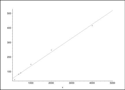
  Figure 1: Dispersions for $\nu_{0}=20$ as a function of $x\equiv\nu_{fin}$

  One can see that it can be approximately the straight line

  $$\delta\nu=42+0.095\nu_{fin}$$

• For $\nu_{0}=50$ one can see the analogous dependence of $\delta\nu$ on $\nu_{fin}$ drawn in Figure 2

  

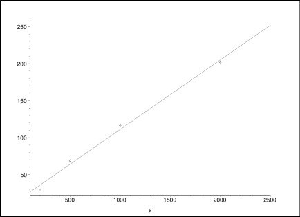
  Figure 2: Dispersions for $\nu_{0}=50$ as a function of $x\equiv\nu_{fin}$

  One can see that it is also approximately the straight line

  $$\delta\nu=17+0.094\nu_{fin}$$

The result of these two numerical pictures is that one can not say that the fluctuations disappear when $\nu$ goes to infinity. The result is that

$$lim_{\nu\rightarrow\infty}\delta\nu=0.095\nu$$

The direct sequence is that one has to take fluctuation effects of growth into account.

Fortunately, the true result is a little bit more optimistic. In reality $\delta\nu/\nu$ becomes small for enough big $\nu$. More precisely the result of mentioned simulations give

$$\delta\nu\sim\nu^{1-\epsilon}$$

where

$$\epsilon\simeq 0.22\pm 0.05$$

It can be seen from corresponding pictures drawn in logarithmic scales. The following Figure 3 shows the dependence of $\ln\delta\nu$ on $\nu$ for $\nu_{0}=20$

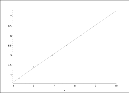
Figure 3: Logarithm of dispersions for $\nu_{0}=20$ as a function of $x\equiv\ln\nu_{fin}$

The linear approximation

$$\ln\delta\nu=0.74\ln\nu-0.76$$

is also drawn.

The same dependence for $\nu_{0}=50$ is drawn in Figure 4

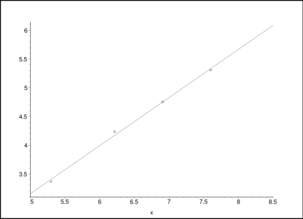
Figure 4: Logarithm of dispersions for $\nu_{0}=50$ as a function of $x\equiv\ln\nu_{fin}$

The best linear approximation

$$\ln\delta\nu=0.83\ln\nu-1.03$$

is also drawn.

So, the convergence $\delta\nu/\nu\rightarrow 0$ formally takes place. But for every concrete (finite) situation one has to take this correction into account.

5 Theoretical explanation for dependence of dispersion on the final size

Here we are interested in the dependence of $\delta\nu$ on $\nu_{fin}$. This dependence will be like a power one and the value of the power has to be determined.

The starting point of explanation will be equation (4). We can see that $D_{r}=\frac{1}{3r^{2}}$ has a singularity at $r=0$. Certainly, $r=0$ is out of range of consideration. At least $D_{r}$ is a rapidly decreasing function. It means that the main blurring takes place in initial period of time of growth (i.e. some $\delta_{initial}r$ has been formed) and later this blurring is mainly translated along $\nu$-scale.

It is rather easy to estimate the role of translation. Really, due to translation

$$\delta\nu=\delta_{initial}r\ (\frac{d\nu}{dr})=\delta_{initial}r\ 3\nu^{2/3}$$

since the value of initial dispersion $\delta r$ is fixed we come to the power like dependence

$$\delta\nu\sim\nu_{fin}^{2/3}$$

The power is $2/3$.

One has also to consider the standard diffusion of purely independent events with blurring in the $r$ scale. This leads to $\delta r\sim r^{1/2}$. Then

$$\delta\nu\sim r^{1/2}=\nu^{1/6}$$

The power like dependence together with scaling invariancy means that some fixed part of evolution forms the dispersion $\delta_{initial}r$. For this value one can take

$$\delta_{initial}\nu\sim r_{initial}^{1/2}=\nu^{1/6}_{initial}$$

Since $\nu_{initial}=\alpha\nu_{fin}$, where $\alpha$ is some fixed parameter, one can come to

$$\delta_{initial}\nu\sim\nu^{1/6}_{fin}$$

and

$$\delta\nu\sim\nu^{1/6}_{fin}(\frac{d\nu}{dr})\sim\nu_{fin}^{2/3+1/6}=\nu_{fin}^{0.83}$$

Numerical simulations confirm this result.

6 Numerical results for dispersion as a function of the initial size

The problem of establishing the dependence of $\delta\nu$ is not yet solved because there exists the uncomfortable dependence of $\delta\nu$ on the starting size $\nu_{0}$.

One can not put $\nu_{0}$ to zero and solve this problem because in numerical simulation one has to exclude the dissolution of embryos.

The simulations with finite $\nu_{0}$ shows the irregular behavior of $\delta\nu$ for small $\nu$. Seeking for the power like dependence we shall draw curves in logarithmic scales. The dependence of $\ln\delta\nu$ on $\ln\nu_{0}$ is drawn in Figure 5 for $\nu_{fin}=1000$ and Figure 6 for $\nu_{fin}=2000$

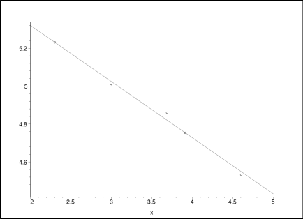
Figure 5: Logarithm of dispersions for $\nu_{fin}=1000$ as a function of $x\equiv\ln\nu_{0}$

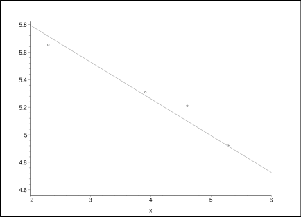
Figure 6: Logarithm of dispersions for $\nu_{fin}=2000$ as a function of $x\equiv\ln\nu_{0}$

The straight lines drawn in these figures are the following

• In Figure 5

  $$y=6-0.3x$$

• In Figure 6

  $$y=6.3-0.27x$$

7 Theoretical explanation of dependence on initial size

Again we are seeking for the power in the power like dependence of $\delta\nu$ on $\nu_{0}$. Having noticed that $D_{r}\sim\nu^{-2/3}$ we can rewrite this equation as

$$D_{r}\sim(t-t^{\prime})^{-2}$$

where $t^{\prime}$ is the moment corresponding to $r$.

We see that $D_{r}$ is mainly concentrated in initial moments of time. This allows us to state that approximately

$$\delta r\sim(\int D_{r}dt)^{1/2}$$

Having calculated the last integral and interested in behavior at the lower limit of integration we come to

$$t^{-1/2}\sim\delta r$$

In terms of $\nu\sim t^{3}$ one can rewrite the last equation as

$$\nu^{-1/6}\sim\delta r$$

The numerical results confirm in general features the small negative value of the power. But the some discrepancy between theoretical model and results of simulation still remains.

Then we have to use the ideas of the self-similarity. There is no difference between $\nu_{0}$ and $\nu_{fin}$. Really, the value $\nu_{0}$ is the final value for the region $[0,\nu_{0}]$ which is out of consideration. The dispersion was supposed to be like $\nu_{0}^{1/2}$. But since $\nu_{0}$ can be interpreted as a final size, we know that dispersion really will be $\nu_{0}^{\frac{1}{6}+\frac{2}{3}}$.

Then we have to increase the power of the previous result in

$$(1/6+1/3)/(1/2)$$

times. This leads to

$$\delta r\sim\nu^{-[(2/3+1/6)/(1/2)]*(1/6)}=\nu^{-5/18}$$

Then the coincidence between theoretical and experimental results becomes satisfactory.

8 Calculations for the kernel

Since the functional dependence on $\nu_{0}$ and on $\nu_{fin}$ have been determined we don’t know only the numerical coefficient in the formula

$$\delta\nu=const\nu_{0}^{-5/18}\nu_{fin}^{5/6}$$

This coefficient can be determined by the unique computer simulation or by application of analytical model to one of the concrete situations.

Here we shall show no more than an illustrative example of calculations. The weak feature is that it does not correspond to all approaches used above.

Let us choose the situation used in simulations for the mean value. The value of dispersion has to be calculated as following:

• The moments of time

  $$t_{0}=3\nu_{0}^{1/3}/\zeta$$ (6)

  and

  $$t_{f}=3\nu_{fin}^{1/3}/\zeta$$ (7)

  have to be determined.

• Dispersion in $r$ scale is

  $$\delta r=\sqrt{2N_{total}}$$

  where $N_{total}$ is the effective total number of events. It cam be approximately calculated according to the following formula

  $$N_{total}=2\int_{t_{0}}^{t_{f}}D_{r}dt$$

  to have an analogy with $\delta r=\sqrt{4Dt}$ in a case $D=const$. Having used (5) and keeping in mind $\delta r\sim\sqrt{4Dt}$ we come to

  $$\delta r=\sqrt{4\int_{t_{0}}^{t_{f}}\frac{1}{9}\frac{\zeta+2}{2}\frac{3^{2}}{\zeta^{2}t^{2}}dt}=\sqrt{2(\zeta+2)\frac{1}{\zeta^{2}}(\frac{1}{t_{0}}-\frac{1}{t_{f}})}$$

• Dispersion in $\nu$ scale will be

  $$\delta{\nu}=\delta{r}*3\nu_{fin}^{2/3}$$

  After substitution of (6) and (7) we come to

  $$\delta{\nu}=3\nu_{fin}^{2/3}\sqrt{\frac{\zeta+2}{\zeta^{2}}(\frac{\zeta}{3\nu_{0}^{1/3}}-\frac{\zeta}{3\nu_{fin}^{1/3}})}\sqrt{2}$$

• It is quite evident that the dispersion of self blurring

  $$\delta_{0}\nu=\sqrt{2(\zeta+2)/\zeta\nu_{fin}}$$

  has not to be added. This is because we have not divided the whole region into two parts but integrate $D_{r}$ over the whole time interval.

The result for dispersion without self blurring will be

$$\delta{\nu}=155$$

The addition of dispersion of self blurring leads to

$$\delta{\nu}\sim 200$$

It practically coincides with the result of simulations.

As the result the dependence of $\delta\nu$ will be

$$\delta\nu=155(\frac{\nu_{fin}}{1000})^{5/6}(\frac{20}{\nu_{0}})^{5/18}$$

9 Application for concrete systems

Decay

Now we shall apply the already known formulas for concrete systems. It is known that two typical types of external conditions are the decay of the metastable state [3] and the so-called dynamic conditions for condensation [4].

The global theories of evolution based on averaged rates of nucleation (formation of droplets) and droplets growth were given in [3] for decay and in [4] for dynamic conditions.

The peculiarities of stochastic appearance of droplets were investigated in [2], [5] for decay and in [6], [7] for dynamic conditions. In these publications the rate of growth for supercritical embryos of liquid phase is supposed to be the regular one.

The results in description of stochastic effects in [2], [5], [6], [7] were achieved by application of algebraic structure of the nucleation period. This structure will be very important below.

In the situation of decay the structure was the following one:

• Until the moment when the prescribed (by recipe of the monodisperse approximation) part of the total (averaged total) number of droplets has been appeared the system simply waits. This is the first subperiod of the nucleation period.

• Then the second subperiod begins. In this period the rest droplets appear. The vapor consumption and, thus, the behavior of supersaturation is fully governed by the growth of droplets appeared in the first subperiod.

• Dispersion of the number of droplets appeared in the first subperiod equals to zero, the system is simply waiting for the appearance of the necessary amount of droplets.

• Dispersion of the rest droplets, i.e. of the number of droplets appeared in the second subperiod equals to the standard dispersion. But due to the fact that the number of the rest droplets is less than the total number of droplets the final dispersion will be less than the standard one.

The number of droplets appeared in the first subperiod will be marked by $N_{first}$. The number of droplets appeared in the second subperiod will be marked by $N_{rest}$.

All conclusions except the last one remain valid also under the stochastic model for the droplets growth. The last conclusion has to be reconsidered. Really, earlier the cut off by the vapor consumption was absolutely regular since the number of droplets in the first subperiod has to be absolutely fixed and, hence, the action of these droplets was absolutely prescribed.

Now the situation is changed. The cut off of the rest part of spectrum can be initiated in different moments of time since the droplets from the first part of spectrum (let us call them as the the leading droplets) can grow faster or slower.

One can illustrate the effect of the different velocity of growth by the following picture

• Suppose that the droplets grow slower than the averaged velocity. Then the moment of the cut off will be later and more droplets than the standard value appear in the rest part of spectrum.

• Suppose that the droplets grow faster than the averaged velocity. Then the moment of the cut off will be earlier and less droplets than the standard value appear in the rest part of spectrum.

We shall call this picture as the ”unbalanced effects of growth” (UEG)

From the effective monodisperse approximation [5] we know the ”initial” size and the final ”size”. The number of droplets in the monodisperse peak in also known.

Certainly, the picture of UEG isn’t absolutely correct. It is clear that the balancing factor appear. This factor is similar to that which leads to the absence of dispersion in formation of the leading droplets.

Suppose that the initially determined leading droplets grow slower than ordinary. Does it mean that only these droplets have to be taken into account in vapor consumption during the nucleation period? Certainly not. We have simply to include into the group of leading droplets some new droplets appeared a few moments later than the initial boundary between the leading droplets and the rest droplets. So, the existence of a balancing force is evident here.

Now suppose that the initially determined leading droplets grow faster than ordinary. Then we have to exclude from the group of leading droplets some the last droplets appeared just before the initial boundary between the leading droplets and the rest droplets. So, the balancing force here also takes place.

It is clear that the picture with unbalanced effects of growth will estimate the stochastic effects of growth from above. We shall use this property to calculate the stochastic effects in this picture and then to see that they are small enough.

In reality the result from stochastic growth will be some times smaller.

Now we turn to the general case of asymptotic of the big number of molecules in critical embryo.

To grasp the stochastic effects from above we use the picture of unbalanced effects of growth and calculate the effects from the stochastic appearance of droplets and from stochastic growth into dispersion. We suppose that one can add dispersions caused by both stochastic causes. It is true at least when one of dispersions is much smaller than another. Namely this situation will take place.

Dispersion of appearance is

$$D_{appear}\sim\sqrt{2N_{rest}}$$

and dispersion of growth will be connected with the fact that the number of the rest droplets $N_{rest}$ will fluctuate.

If we forget that $N_{rest}$ is the argument of the square root which smoothes the result we will get the estimate from above. So, we will forget.

So, we will calculate the dispersion $\delta_{1}$ of one droplet caused by stochastic growth from the size $\nu_{st}$ up to the final size.

Fortunately the initial size is well determined in the advanced monodisperse approximation and it is not zero. In the previous initial monodisperse approximation it was zero and the consideration of stochastic effects required to give in [5] a new version where the initial position of monodisperse spectrum (the $z$ -coordinate) in renormalized scale is $0.4-0.336$. Namely the new version has to be used.

So, the value of $\nu_{0}$ for all droplets in the monodisperse spectrum will be

$$\nu_{0}^{1/3}=(0.4-0.336)\nu_{fin}^{1/3}$$

One can also determine $\nu_{0}$ in a following simple manner. The actual height of monodisperse spectrum is the unperturbed rate of nucleation (of appearance) $J_{0}$. Since

$$N_{first}\approx J_{0}\delta r$$

we can get the characteristic width of the spectrum $\delta r$. This value will be initial value for $\nu_{0}^{1/3}$. It is clear that approximately this way leads to the same value of $\nu_{0}$. Then since the dependence on $\nu_{0}$ is like $\nu_{0}^{-1/6}$ we see that the results of two ways to determine $\nu_{0}$ will be approximately equivalent.

The zero value of $\nu_{0}$ would lead to divergence, now such a danger is over and one can see that the asymptotic at $\nu\rightarrow\infty$ for characteristic relative deviation in $\nu$ is

$$\delta\nu=\nu_{fin}^{5/6}/\nu_{fin}^{5/18}$$

and goes to zero. The total characteristic relative deviation will be

• for one droplet in the monodisperse peak

  $$D_{unbal}\sim\nu_{fin}^{5/6}/\nu_{fin}^{5/18}$$

• for all droplets in the monodisperse peak

  $$D_{unbal}\sim\nu_{fin}^{5/6}/\nu_{fin}^{5/18}*1/\sqrt{N_{first}}$$

It will be many times less than the relative dispersion

$$D_{stoch}\sim 1/\sqrt{N_{rest}}\sim 1/\sqrt{N_{first}}$$

of the number of droplets caused by stochastic appearance.

We have to note the absence of the shift of the averaged value of the final size from the value calculated on the base of the regular law of growth. The order of this deviation is less than the characteristic attained value. If this shift was essential the action on the averaged number of droplets would be significant.

One has to note that the in last remark the regular law means the regular discrete law and the main effects will be the effects of discrete character of the droplets growth.

Dynamic conditions

In dynamic conditions all previous arguments are valid. The initial size $\nu_{0}$ has to determined by the following way. Since in the approximation of monodisperse consumption [7] the monodisperse spectrum is formed already at $z=-3/c$ one can say that it is formed at the ideal conditions (the real supersaturation coincides with the ideal one). Then the characteristic width of spectrum will be $c^{-1}$. Then the starting value value $\nu_{0}^{1/3}$ will have the order $c^{-1}$

$$\nu_{0}^{1/3}\sim c^{-1}$$

The final value $\nu_{fin}^{1/3}$ will have the order $(3\div 4)c^{-1}$

$$\nu_{fin}^{1/3}\sim(3\div 4)c^{-1}$$

All other constructions are absolutely analogous.

Certainly, the numerical simulation can not give correction terms where the effects of stochastic growth can be noticed because these effects will be corrections for corrections to the main result. The corrections connected with the discrete growth by steps of absorption of one molecule will be more significant.

One has also to note that at the further periods of evolution (after the end of nucleation) the stochastic effects of growth will be more important. This consideration will be presented in a separate publication.

References

- [1] Kurasov V., The form of embryos sizes in the first order phase transitions, Theoretical and Mathematical Physics, vol. 131, number 3 , p.503-528
- [2] Kurasov V., Preprint cond-mat/0410616, Explicit two cycle model in investigation of stochastic effects in diffusion regime of metastable phase decay, 61 p.
- [3] Kuni F.M., Novojilova T.Yu., Terentiev I.A., Kinetics of heterogeneous nucleation under the instantaneous creation of initial supersaturation. Russian Journal of Theoretical and Mathematical Physics, v.60, p.276, (1990)
- [4] Kurasov V.B., Phys. Rev. E, vol.49, p.3948 (1994)
- [5] Kurasov V., Preprint cond-mat/0410774, Monodisperse approximation as a tool to determine stochastic effects in decay of metastable phase, 19p.
- [6] Kuirasov V., Preprint cond-mat/0412142, Corrections to a mean number of droplets in nucleation, 27 p.
- [7] Kurasov V., Preprint cond-mat/0412141, Dispersion of nucleation under the smooth variation of external conditions, 25 p.