Clauser-Horne inequality and decoherence in mesoscopic conductors
Elsa Prada
Departamento de Física Teórica de la Materia
Condensada, C-V, Universidad Autónoma de Madrid, E-28049 Madrid,
Spain
Institut für Theoretische Festkörperphysik,
Universität Karlsruhe, D-76128 Karlsruhe, Germany
Fabio Taddei
NEST-INFM & Scuola Normale Superiore, I-56126 Pisa, Italy
Rosario Fazio
NEST-INFM & Scuola Normale Superiore, I-56126 Pisa, Italy
Abstract
We analyze the effect of decoherence on the violation of the
Clauser-Horne (CH) inequality for the full electron counting
statistics in a mesoscopic multiterminal conductor. Our setup
consists of an entangler that emits a flux of entangled
electrons into two conductors characterized by a scattering matrix
and subject to decoherence.
Loss of phase memory is modeled phenomenologically by introducing fictitious extra leads.
The outgoing electrons are detected
using spin-sensitive electron counters. Given a certain average
number of incoming entangled electrons, the CH inequality is
evaluated as a function of the numbers of detected particles and on
the various quantities characterizing the scattering matrix. When
decoherence is turned on, we show that the amount of violation of
the CH inequality is effectively reduced. Interestingly we find
that, by adjusting the parameters of the system, there exists a
protected region of values for which violation holds for
arbitrary strong decoherence.
Besides its generation, a crucial issue is that of the detection of
entanglement. By means of a beam-splitter, entanglement can be
detected in transport through an analysis of current noise
burkard00 or higher cumulants taddei02 . Furthermore,
the presence of entanglement can be revealed by analyzing the Bell
inequality and quantities like concurrence wootters98 , which
have been expressed in terms of zero-frequency charge and
spin-current noise
kawabata01 ; lesovik01 ; chtchelkatchev02 ; samuelsson03 ; beenakker03 ; beenakker04-2 ; sauret04B .
Violation of a Bell inequality implies that there exist quantum
correlations between the detected particles that cannot be described
by any local hidden variables theory. In the same spirit as it was
done for the noise, in Ref. faoro04, a Clauser-Horne(CH)
inequality clauser74 ; mandel95 was derived for the Full
Counting Statistics (FCS) of electrons and its properties were
discussed newnota2 . In particular, it was found that the
maximum violation of the CH inequality for electrons in the Bell
state simply scales as the inverse of the number of injected
particles. It was also found that the CH inequality is violated for
a superconducting hybrid structure and, more interestingly, for a
three terminal fully normal device.
In real systems electrons are unavoidably coupled to the
electromagnetic environment. As a result dephasing takes place,
thereby reducing and eventually destroying entanglement.
Understanding the consequences of dephasing is an important issue.
In Refs.
samuelsson03, ; samuelsson03-2, ; samuelsson04, ; samuelsson04-2,
the effect of dephasing was mimicked by introducing in the density
matrix of the electronic entangled states a phenomenological
parameter which suppresses its off-diagonal elements. By properly
choosing the transmission probability of beam-splitters or tunnel
barriers, violation of Bell inequality was found even for “strong”
dephasing. In Refs. beenakker03, ; beenakker03-3, dephasing
was introduced averaging over an uniform distribution of random
phase factors accumulated in each edge channel of the quantum Hall
bar. If the two edge channels are mixed by the tunnel barrier, no
violation was reported for “strong” dephasing. The effect of
decoherence and relaxation has also been analyzed using a Bloch
equation formalism in Ref. burkard03, .
In the present work we analyze the CH inequality for the FCS
faoro04 in the presence of dephasing. We consider the
prototype setup depicted in Fig. 1, consisting of a generic
entangler connected to two conducting wires. Entangled electrons
injected in the two leads are detected by performing spin-selective
counting along a given local quantization axis. The entangled
electrons are subject to decoherence while transversing the
conductors (thus before reaching the detectors)newnota1 .
Various phenomenological methods have been developed to treat
dephasing in transport through mesoscopic conductors. In Refs.
seelig01, ; marquardt04, , which actually describes exactly
nonequilibrium radiation acting on the system, dephasing is induced
by a classical fluctuating potential. In Ref. pala04, ,
dephasing is treated as random fluctuations of the phase of
propagating modes through the conductor. Both methods have been
recently applied to FCS in Refs. pala04-2, ; forster05, . In
this paper decoherence is introduced as due to the presence of
additional fictitious reservoirs along both wires. This method,
which mimics the effect of inelastic processes, was introduced by
Büttiker buttiker86 ; buttiker88 in terms of fictitious extra
leads nota1 . The advantage of this model resides in the fact
that inelastic, phase randomization processes are implemented within
an elastic, time-independent scattering problem. In the rest of the
paper we shall refer to decoherence as to the effect produced by
such fictitious additional leads.
As expected, we find that decoherence suppresses the violation of
the CH inequality, though leaving unchanged the range of angles for
which violation occurs. In particular, the value of the maximum
violation is suppressed more rapidly as compared with the absence of
decoherence (exponentially with the square root of the number of
injected electrons instead of algebraically). Importantly, by
studying the CH inequality as a function of the number of
transmitted electrons, there exist values of such quantity that are
more protected against decoherence.
The paper is organized as follows: In Section II we
described in detail the mesoscopic system we are considering to test
the violation of the CH inequality together with the
phenomenological model of decoherence. Section III is
devoted to the formulation of the CH inequality for the FCS within
the scattering approach and to the analysis of the no-enhancement
assumption (Section III.1). The results are presented in
Section IV, where a systematic analysis of the
violation of the CH inequality against all the parameters of the
device is addressed. A concluding summary is provided in Section
V.
For completeness, we include in Appendix A the results
relative to an asymmetric setup, whereby decoherence occurs only in
one of the two wires. In Appendix B and
C we collect, respectively, the expressions
of the expectation values and the different probability
distributions.
II Description of the system
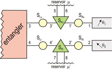
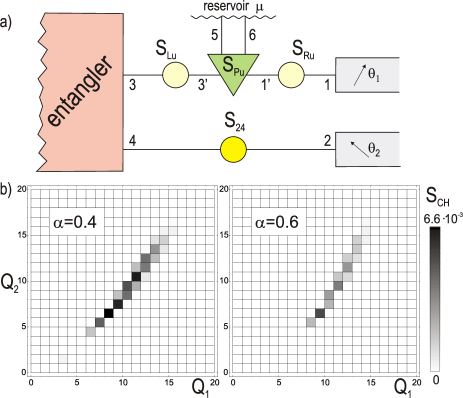
Figure 1: (Color online) Idealized setup for testing the CH
inequality for electrons in a solid-state environment in the
presence of decoherence. It consists of three parts: An entangler
that produces pairs of spin-entangled electrons exiting from
terminals 3 and 4. Two conductors that connect these terminals with
exiting leads 1 and 2, and two analyzers. The conductors are
described by the elastic scattering matrices and , and the inelastic
ones and . These last ones can
simulate phenomenologically the presence of decoherence through the
coupling via two leads ( and ) to two additional
reservoirs of chemical potentials and . Electron
counting is performed in leads 1 and 2. Finally, and
are the angles at which the spin-quantization axis are
oriented.
We consider the setup illustrated in Fig. 1. It consists of
an entangler, two conducting wires and two spin-selective
counters. The entangler, on the left-hand-side, is a device that
produces pairs of electrons, with energy , in a
maximally spin entangled state (Bell state). On the right-hand-side
of Fig. 1 the electron counting is performed in leads 1 and
2 (at equal electrochemical potential ) for
electrons with spin aligned along the local spin-quantization axis
at angles and (spin-selective counters). As a
convention we say that the analyzer is not present when the electron
counting is spin-insensitive (electrons are counted irrespective of
their spin direction). Since we assume no back-scattering from
counters to the entangler, the particles which are not counted are
lost and hence there is no communication between the two detectors.
Leads 3 and 4 of the entangler are connected to exit leads 1 and 2
through two conductors, where inelastic processes are introduced
through the fictitious lead model of Büttiker buttiker84 . Let
us analyze in detail the upper wire (see Fig. 1) which
connects the emitting lead with the exiting lead . The
conductor consists of three scattering regions. The elastic
scatterer connecting lead 3 to 3’ is described by the matrix
(1)
[The index L (R) stands for Left (Right) elastic scatterer, while P
stands for Probe scatterer; u (l) refers to the upper (lower) wire.]
Here () is the probability amplitude for an
incoming particle with spin from lead 3 to be reflected
(transmitted into lead 3’). For a normal single-channel wire we set
, and
, where is the
transmission probability. Inelastic scattering is introduced by
plugging in an additional reservoir of chemical potential with
an energy- and spin-independent scattering matrix
(2)
represented by a triangle in Fig. 1. For the sake of
clarity, we have denoted by a check (), a caret
() and an overbar (), respectively, (22),
(44) and (88) matrices. In Eq. (2)
and are, respectively, unit and zero
(22)-matrices in the spin space, and is the
probability for transmitting a particle between leads 3’ and 1’. The
coupling parameter ranges from , when no particles are
transmitted into leads 5 and 6 from leads 3’ and 1’, to ,
when no particles are transferred between leads 3’ and 1’. A third
elastic scatterer, described by a matrix ,
connects lead 1’ to lead 1. The conductor is therefore described by
the matrix defined as
, where the notation stands for the
scattering matrix composition (elimination of internal current
amplitudes) datta95 . For simplicity, we shall assume that
.
Due to the presence of the additional reservoir,
particles propagating through lead 3 are transmitted partially to
lead 1 and partially to leads 5 and 6 (see Fig. 1). The
additional reservoir, however, can transfer itself particles to lead
1 and 3. As a result, only a fraction of the particles arriving in
lead 1 comes from coherently transmitted ones sent in from
lead 3, with probability
(3)
Another fraction, the incoherent contribution, comes from the
additional reservoir through leads 5 and 6, with probability
(4)
The presence of the extra reservoir mimics the fact that the current
flowing through the conductor is partially composed of particles
(the incoherent fraction) which have lost phase memory while
traversing it. For all particles are coherently
transmitted and , while for all
particles are transferred incoherently and . For
, the overall transmission probability through the
conductors is given by . In the rest of the paper
we will refer to as to the decoherence rate.
The chemical potential of the additional reservoir is set in
such a way that no net current flows in or out of the reservoir
(). This constraint is enforced only on average. An
instantaneous current in or out the additional reservoir is then
allowed buttiker86 ; buttiker88 ; beenakker92 ; blanter00 , and a
non-fluctuating chemical potential is assumed (for this reason
the additional terminal does not behave as a voltage probe).
A similar description applies to the lower wire connecting lead 4
with lead 2, so that the scattering matrix of the conductor is
defined as , where, for
simplicity, we set . If the
angles and of the analyzers are parallel to
each other and in the absence of spin mixing processes, the total
matrix of the system can be written as
(5)
The general scattering matrix relative to non-collinear angles
is obtained from by rotating
the spin quantization axis independently in the two conductors (note
that this is possible because the two wires are decoupled) brataas01 :
, where is the rotation
matrix given by
(6)
and
(7)
For simplicity, we further assume that the two conductors are equal
and that they are subjected to the same degree of decoherence, so
that . For this reason the chemical
potentials of the additional reservoirs are identical. It is
interesting to notice that decoherence processes in the two wires
are, in some sense, ”uncorrelated”, meaning that we have imposed
that the currents flowing through the fictitious leads vanish
separately in the two reservoirs.
(Correlations can be introduced, for example, by imposing .) In the symmetrical
setup we are considering here,
. In the
rest of the paper we consider the case in which all the reservoirs
are at zero temperature.
The incoming state of the system depends on whether the
energy of electrons falls within the range
or :
(8)
where
(9)
and
(10)
In Eqs. (9) and (10) is
the creation operator for a propagating electron in lead with
spin at energy . The upper sign refers to the case in
which the incoming state is a spin triplet and the lower sign to the
spin singlet. Electrons with energy between and
are exiting leads and of the entangler in
a superposition of spin and states. For
energies between and electrons are also
injected from the additional leads (with indexes 5, 6, 7 and 8) in a
factorized state. Note that this occurs only in the presence of
decoherence, i.e. for .
By setting and , the total
current flowing in lead 1, calculated using the Landauer-Büttiker
formalism landauer57 in the linear response regime, is given
by
(11)
Although the coherent part of the current decreases with ,
the total current increases with it (except for , where it
remains constant and equal to ). We would like to mention
that this is a special feature of the model of decoherence we are
using, not to be expected in general.
III CH Inequality for the Full Counting Statistics
The quantity employed in the formulation of the CH inequality, as
derived in Ref. faoro04, , is the joint probability
for transferring a number of and electronic
charges into leads and over an observation time . The CH
inequality is based on the hypothesis that the outcome of a
measurement could be accounted for by a local hidden variable
theory. The test of the CH inequality proceeds as follows. The
entangler is switched on during an observation time (where the
minimum is the inverse of the measuring device bandwidth) in
which it emits an average number of pairs of entangled
electrons. After traversing the conductors (and being affected by
inelastic scattering) the electrons are counted in both terminals 1
and 2. The experiment is then repeated to get single terminal and
joint terminal probability distributions that particles arrive
into analyzer 1 and particles arrive into analyzer 2 (along a
local spin-quantization axis or independently of it) with
.
The possible violation, or
the extent of it, also depends on and .
is the joint probability in the
presence of two analyzers, where electrons are counted in
lead 1 along direction and are counted in lead 2
along . is the corresponding
joint probability when one of the two analyzers has been removed.
The same notation will be used for single terminal probability
distributions: in the presence of an analyzer
and if no analyzer is present. Eq. (12)
holds for all values of and which satisfy the no-enhancement assumption:
(13)
The joint probability distribution for transferring
electrons with spin in lead 1, electrons with spin in lead 2 and so on is given by
(14)
where
is its characteristic function that can be expressed within the
scattering approach.
For long measurement times , the total characteristic function
is the product of contributions from different energies, so
that
(15)
The energy-resolved characteristic function for the transfer of
particles at a given energy in a structure attached to leads
can be written as muzykanskii94 ; levitov93 ; levitov96
(16)
where the brackets stand for the quantum
statistical average over the thermal distributions in the leads.
Assuming a single channel per lead, is
the number operator for outgoing (incoming) particles with spin
in lead and ,
are vectors of real numbers, one
for each open channel. In terms of outgoing (incoming) creation
operator
(), which are linked by the total
scattering matrix of the system , the number operators can be
expressed as
(17)
At zero temperature, the statistical average over the Fermi
distribution function in Eq. (III) simplifies to the
expectation value calculated over the state defined in
Eq. (8). The interval of integration in Eq. (15)
can be separated in two energy ranges, namely and
. Since, in the limit of a small voltage bias ,
is energy-independent, Eq. (15) can be
approximated to
(18)
where and .
According to Eq. (III), both single terminal and joint
probability distributions require the computation of
multidimensional integrals, which can only be performed numerically.
In Appendix C it is shown that the various
probability distributions needed to evaluate the CH inequality can
be expressed in a differential form, more suitable for numerical
evaluation. All the expectation values needed for the calculations
are collected in Appendix B. Since the two wires
are decoupled and there are no spin-flip processes, the joint
probabilities with a single analyzer are factorized:
(19)
Rotational invariance makes and
independent of the angle of the analyzers,
while depends on the angles only
through the combination (upper sign
for triplet and lower sign for singlet), so that we can define
and . As a result, the CH inequality depends
only on three angles ,
and
( is a linear combination of the
other three: ). Since
is an even function of
, in order to find maximal
violations we can restrict the evaluation of the CH inequality to
the following set of angles:
. (This is found
by imposing that positive contributions to
are maximum while negative contributions are minimum.) The quantity
, characterizing the CH inequality, will
therefore depend on a single angle , on the decoherence
strength and on the value of the transmitted charge
and . As a result, the CH inequality takes the simplified form
(20)
Without loss of generality we can choose .
The other cases can be recovered by rotating the polarizers an angle
.
III.1 No-enhancement assumption
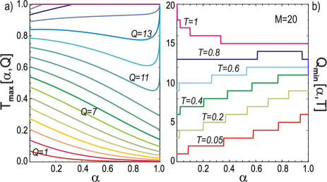
Figure 2: (Color online) a) Maximum value of the transmission,
, allowed by the no-enhancement assumption as a
function of decoherence rate for emitted pairs and
for the different values of . b) Minimum allowed number of
transmitted particles for a fixed wire transmission
as a function of the decoherence rate.
As mentioned above, the CH inequality can be derived under the
no-enhancement assumption, Eq. (13). Such a
condition is trivially true when a single particle is transmitted,
: The presence of an analyzer can only decrease the counting
probability clauser74 . However, when many particles are
transmitted, , the no-enhancement assumption is a relationship
between distribution probabilities that is not, in general,
satisfied for all values of .
We remind that in the absence of decoherence faoro04 , for
given and , the no-enhancement assumption in one of the two
leads is satisfied only within a range of values of below
certain threshold . In the case of different
numbers of transmitted particles in lead 1 and 2 (),
the maximum allowed transmission probability must be taken to be the
minimum between and ,
according to our assumption of identical wires.
The no-enhancement assumption is affected by decoherence as a
consequence of the fact that single terminal probabilities, with or
without analyzer, depend on . More precisely, the
no-enhancement assumption in one of the two leads is satisfied for
transmissions up to a threshold value which is now a function of
: . Unlike the ideal case, for
it is not possible to find an analytical expression
for . In Fig. 2a is
plotted as a function of for and all values of
from 1 to 20. One can see that monotonically
decreases with for values of and
monotonically increases for large values of . For intermediate
values of , decreases up to values of
close to one and then rapidly increases reaching one when
. This behavior is specific of the fictitious lead model
and reflects the fact that both the average total current
[Eq. (11)], related to , and the average spin-polarized
current, related to , are increasing functions of
. Indeed, as a consequence of a finite , the two
distributions shift to larger values of , as it would happen for
an enhanced effective transmission probability. Its maximum allowed
value by the no enhancement assumption is therefore reached for a
smaller . As a consequence must decrease with
. This argument is not valid when
at , since the average currents do not change appreciably
with and only the peculiar shape of the distributions
matters. We define
(21)
Alternatively, given a wire with a fixed transmission , the
no-enhancement assumption is verified for values of bigger than
or equal to a certain value . For
, the behavior of is shown in
Fig. 2b for and for different transmissions.
We observe that it increases (step-wise, since only integer values
of the number of particles are permitted) as a function of the
decoherence rate for almost every transmission , except for those
close to unity, for which it decreases. The behavior for small
values of can still be understood in terms of the average
current increase with . For , being
at , decoherence can only cause a decrease.
IV Results
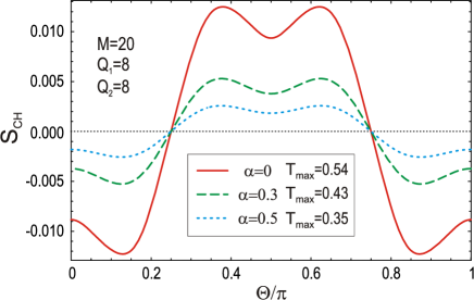
Figure 3: (Color online) The quantity is
plotted as a function of for , and
different decoherence rates at the corresponding maximum allowed
transmissions. In particular, for (solid line)
, for (dashed line)
and for (dotted line)
. The amount of violation of the CH inequality
decreases with , whereas the range of angles for which
violation occurs does not change. We call the
angle corresponding to the maximum violation.
In the present section we shall discuss how the CH inequality of
Eq. (20) is affected by the presence of decoherence.
There are some general characteristics of the behavior of that were already found in the absence of
decoherence faoro04 that hold also for finite
nota . The most relevant are the following:
•
is always symmetric as a function of around
;
•
for given , and the maximum violation always occurs for .
In Fig. 3, is plotted as a
function of the angle for and . The three
curves refer, respectively, to (solid line),
(dashed line) and (dotted line), each one calculated
for the corresponding reported in the label box.
The plot shows that the CH inequality is violated within a certain
window of values of . The violation is suppressed with
increasing decoherence rate, but occurs for the same range of
angles. This is due to the following properties of the joint
probabilities, which hold at for all values of
: i)
,
as a consequence ;
and ii) ,
, for . We checked that by reducing from , but
keeping constant, both the window of angles where violation
is present and its amount are decreased. Note that between
and , there is always an angle for which is maximum, we shall denote it by
. For given , ,
and , the maximum violation occurs at
and .
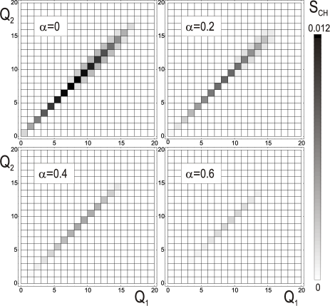
Figure 4: Density plots of the maximum value of , evaluated at
and , in the
() plane for relative to four different values of
decoherence (, , , ). is the maximum violation for
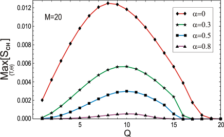
found in the absence of decoherence. Figure 5: (Color online) Maximum value of the quantity ( and
) as a function of for and
different values of decoherence: , , , .
The largest violation always occurs in the absence of decoherence
and, for a given , violation is reduced monotonically with
. The position where the maximum occurs, ,
slightly increases with . At ,
for , for
, for and
for .
We now analyze the maximum violation of the CH inequality for a
given with and
as a function of and . In Fig. 4 we
show four density plots of in the
() plane for different values of decoherence rate and
. In the gray scale white corresponds to and black to its maximum value taken in the
absence of decoherence. When , the CH inequality is
strongly violated for diagonal terms of the distribution (where
). However, some weaker violations are also possible for
, though they tend to disappear with increasing
.
By increasing the values of the plots show that the maximum
violation of the CH inequality decreases rapidly: for
we get only of the largest value reached at . The
behavior of the CH inequality is symmetrical with respect to the
exchange of with for any rate of decoherence. In
Fig. 5 we report the section of the plots in
Fig. 4 along the diagonal of the -plane. The
four curves are relative to , 0.3, 0.5 and 0.8 an .
Several observations are in order. If we denote with
the position of the maximum of a curve, for all
values of decoherence rate , more
precisely, for and
for all other curves. This slight increase of
with is due to the fact that an increase
in decoherence is accompanied by a slight enhancement of the average
current [Eq. (11)] flowing through the wires (as mentioned at
the end of Section II). This is, however, a specific
feature of the model of decoherence we are considering. Note
furthermore that, as decoherence gets stronger, the range of values
of for which violation takes place shrinks.
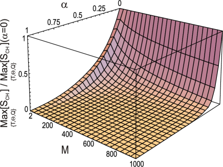
Figure 6: (Color online) , normalized to its
value in the absence of decoherence and calculated at
, and
, is plotted as a function of decoherence rate
and number of injected entangled pairs . Longer
measuring times (i.e. larger values of ) make decoherence more
effective, that is, make the detection of entanglement more
difficult.
We now discuss the violation of the CH inequality as a function of
and at ,
and . In
Fig. 6 the ratio
(i. e. the quantity normalized to its value
in the absence of decoherence) is reported in a three-dimensional
plot as a function of and the number of emitted pairs .
The most interesting feature is that such a ratio decays more
rapidly with as is increased. This means that
decoherence is more disruptive, as far as detection of entanglement
is concerned, for long measuring times (i.e. large ). As an
example, for the extent of the violation is reduced by
at . More precisely, for values of larger
than , we find that the normalized
follows the law:
(22)
with and .
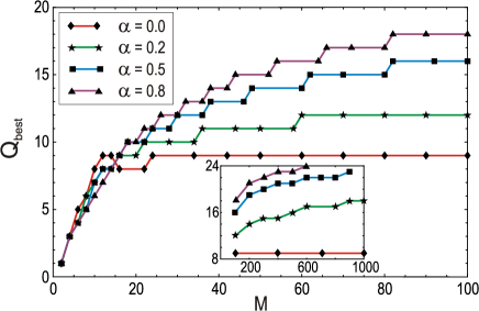
Figure 7: (Color online) is plotted as a function
of for different values of decoherence rate (, 0.2,
0.5 and 0.8). In the inset, curves are shown over an extended range,
up to . For a given , with increasing the value
of increases very slowly remaining of the order of
10.
Another interesting aspect is related to which, as
mentioned above, only slightly increases with for all
values of . As is increased, the value of ,
for a given , does not increase proportionally to , but
very much slowly and surprisingly remains of the order of 10 for
(see Fig. 7). For this can be
understood as follows. On the one hand, one expects
, corresponding to the largest , to be about the position of the maximum of joint
probability distributions, which can be assumed to be equal to the
product . On the other hand, is a decreasing
function of , in fact it decays as faoro04 . The
product is therefore expected to be a constant.
Indeed, it is possible to show, in the large expansion, that
for and
for ,
while for and
for . As a result,
is roughly constant as a function of and
nota0 .
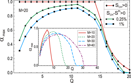
Figure 8: (Color online) Maximum value () of the
decoherence parameter for which there is still violation of the CH
inequality as a function of for . The line with
represents with : from to violation is found for any
decoherence rate. The line with is instead computed using
a threshold which corresponds to of the
maximum violation value for , and the line with
using corresponding to . The
latter threshold is used in the inset where
is plotted for , , and . Interestingly we found
that there is a value that is more robust against
decoherence. In particular, for , for
, for and for . With
increasing , diminishes slowly.
The final point we address is the maximum decoherence rate,
that we denote by , for which there is still violation
of the CH inequality
as a function of . In Fig. 8 we plot
as a function of for at
and . The line with
the symbol shows that violation of the CH inequality
is found for any rate of decoherence for to and
thereafter decreases sharply. Nevertheless,
the extent of violation for close to 1 is almost negligible
for most of . One can therefore introduce a small
positive threshold which defines the
violation as: . The
line with refers to a threshold of of the
maximum value of at ( for ), and the line with
to a (
for ). The latter percentage is used for the thresholds of the
plots in the inset of Fig. 8, where
is plotted for , , and . It
is shown that there are values of that are more resistent to
decoherence, i. e. for which violation survives for larger
decoherence rates. In the caption of Fig. 8, the most
protected value against decoherence is denoted with .
V Conclusions
In this paper we have studied the effect of decoherence on the
violation of the CH inequality formulated in terms of the FCS
faoro04 . The system under investigation (Fig. 1)
consists of an idealized entangler connected, through a pair
of identical mesoscopic wires, to spin-selective counters. We have
assumed that decoherence, which occurs equally but independently in
the two conductors, is produced by the presence of additional
fictitious reservoirs according to the phenomenological model of
Büttiker buttiker86 ; buttiker88 . Decoherence is
parameterized by the rate .
As expected, decoherence gives rise to suppression of the violation
of the CH inequality. The extent of such a suppression has been
analyzed as a function of the parameters which characterize the
system, namely the transmission of the wires, the angle between
analyzers , the number of injected entangled pairs and
the number of transmitted particles and in the counters.
First we have discussed the no-enhancement assumption, a
condition that needs to be satisfied in both leads 1 and 2 in order
for the CH inequality to hold. We have found that such condition, in
a given lead, is verified for all transmission up to some
maximum value which depends on , and, of course,
. In particular, decreases with the decoherence
rate up to some value of and thereafter increases.
The main results can be summarized as follows:
•
Maximal violation, even in the presence of
decoherence, occurs at the largest allowed transmission
and for (it disappears very rapidly
when ).
•
As long as , the angle range of the analyzers for which violation takes place does not depend on
the decoherence rate, though the extent of violation decreases with
.
•
In the absence of decoherence, the maximum violation of the
CH inequality was proved to decay as faoro04 . Here we
have found that, for finite , the parameter decreases exponentially with , more
precisely as , i.e. decays both with
increasing and .
•
The value of for which maximum violation occurs is virtually independent of , which means that the largest violations appear for relatively small numbers of transmitted particles, even at large observation times.
•
Interestingly, we have found that the largest
decoherence rate for which the CH inequality is violated (within a
given small tolerance) presents a maximum as a function
of . This means that there exist numbers of transmitted charges which are
more protected against decoherence, i.e. the influence of the
environment is less disruptive as far as the violation of CH
inequality is concerned.
Although, in this paper, dephasing is assumed to be produced by the
presence of additional reservoirs, other different sources of decoherence
are possible in mesoscopic systems. We believe that this model
captures the main effects of decoherence, as far as violations of
the CH inequality in a mesoscopic system is concerned, and that the
results found in this work may be useful to design the best
experimental conditions.
Since real systems cannot be perfectly shielded from the
environment, the issues analyzed in this work seem adequate not only
from a fundamental point of view, but also in what it might
contribute to the understanding of the properties of lossy quantum
channels. For the future it would be interesting to apply our method
to realistic systems, like normal or superconducting beam splitters.
Of interest would also be the combined effects of the presence of
spin-flipping processes and decoherence.
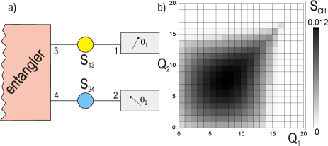
Figure 9: (Color online) a) Idealized setup with a single additional
reservoir in the upper branch of the system. Scattering matrices are
chosen so that, in the absence of decoherence, the two conductors
have equal transmission. b) Density plot of the maximum value of
in the ()-plane for and for
(left) and (right). As decoherence
increases, the maximum violation is not achieved on the diagonal,
but is shifted towards the right-bottom part of the plane
(). This occurs because only the current flowing through
the conductor affected by decoherence is modified. Furthermore, the
suppression of the violation by is less pronounced with
respect to the case with two additional reservoirs. For example, for
we find
achieved at . For and one additional
reservoir we have
reached at , whereas for two additional reservoirs we get
at . For
and one additional reservoir, at , and with two additional
reservoirs, at
. Finally, for and one additional reservoir,
at , and with
two additional reservoirs, at . Figure 10: (Color online) a) Idealized setup with no decoherence but
differently transmitting upper and lower conductors. b) The density
plot of the maximum value of the quantity
is shown in the -plane for .
Acknowledgements.
The authors would like to thank F. Sols for encouraging this work,
P. San-Jose for useful discussions and M. Büttiker and C.W.J.
Beenakker for comments on the manuscript. This work was supported by
the FPI program of the Comunidad Autónoma de Madrid, the EU under
the Marie Curie Research Training Network, EC-RTN Nano, EC-RTN
Spintronics and EC-IST-SQUIBIT2.
Appendix A Asymmetric setup: one additional reservoir
It is interesting to consider the case in which decoherence affects
the two wires differently. In this appendix we study the case when
decoherence affects only one of the two conductors, i.e. in the
presence of a single additional probe, for example, in the upper
branch, as depicted in Fig. 9a. Being the
transmission of the elastic scatterers in the upper conductor, we
choose the transmission of the lower conductor to be equal to
, in order for the two conductors to have the
same conductance in the absence of decoherence.
Fig. 9b shows the density plot of the maximum value of
(with and
) as a function of and , for
, (left) and (right). In the
presence of decoherence the maximum violation is not achieved on the
diagonal (), i.e. the behavior of is not
symmetrical anymore with respect to and . This is due to
the fact that, as we have seen above, the overall current increases
with so that it is more likely to transmit a larger number
of particles in the conductor subjected to decoherence. Another
difference with respect to the case with two additional reservoirs
is that the suppression of the violation by is less
pronounced.
The asymmetry found in the behavior of the density plots of
Fig. 9b must not be confused with the asymmetry we
would obtain in a setup without decoherence but with conductors of
different resistance (system sketched in Fig. 10a). In
this case, by applying separately the no enhancement assumption to
the two conductors, large violations occur in a vast region of the
-plane, as shown in Fig. 10b.
Interestingly, we note that one would get large violations of the CH
inequality for . However, this asymmetry would not come
from the fact that entanglement is weakened by dephasing in only one
wire.
Appendix B Expectation values
The most general expression for the characteristic function when
spin- electrons are counted in lead 1 and spin-
electrons are counted in lead 2 is
(23)
for each relevant energy range: and . When both
spin species are counted in one of the terminals, the characteristic
function reads
(24)
for counting both spins in terminal 1, where we have set .
Using Eqs. (III), (18) and
(23), at zero temperature, one can calculate the
single terminal probability distribution:
(25)
where .
After integration over we get
(30)
If one chooses and , one
obtains and . Therefore,
in order for to be integer, must be an even number.
Using Eqs. (III), (18) and
(24), the single terminal probability distribution
when both spin species are counted in the terminal is
(31)
where .
In the following subsections we collect all the expectation values needed to work
out the expressions for the probability distributions of Eq. (20).
B.1 Setup with two additional reservoirs
Let us consider the setup depicted in Fig. 1, where two
additional reservoirs are present. The expectation values for energies
as a function of transmission , decoherence parameter
and analyzers’ angle are
(32)
(33)
(34)
(35)
(36)
(37)
The expectation values for energies are
(38)
(39)
(40)
(41)
(42)
(43)
B.2 Setup with one additional reservoir
Let us now consider the asymmetrical setup of Fig. 9,
where there is only one additional reservoir. For energies we
have that ,
and
are equal to the case with two fictitious reservoirs. The other
expectation values are
(44)
(45)
(46)
(47)
(48)
(49)
(50)
For energies we have that , , , , and are equal to the case with two additional reservoirs.
The other expectation values are
(51)
(52)
(53)
(54)
Appendix C Probability distributions
In order to calculate the various probabilities needed to evaluate
the CH inequality, Eq. (12) and (20), it is
necessary to solve the integrals of Eq. (III), where the
different characteristic functions are given in
Eq. (23) and Eq. (24). As we
mentioned in Section III, explicit expressions of the
probability distributions in terms of sums are lengthy and
complicated for practical calculations. It is possible,
nevertheless, to express the result for the various probabilities
in a quite simple fashion, which makes them manageable for
computational analysis. The point is to realize that the
characteristic functions are nothing but polynomial functions on the
variables of different degrees. The effect of each
integral of Eq. (III), together with its accompanying
complex exponential , is simply to select
the coefficient of the characteristic function polynomial which
corresponds to the power equal to . Consequently, the result of
the integrals for the various probabilities can be expressed in
terms of order derivatives of the characteristic function, as
we show below. Note that, whenever both analyzers are present, we
will choose without loss of generality: and
. For single terminal probability distributions we
will also set for lead 1 and
for lead 2, although resulting expressions will not depend either on
the direction of the spin or on the angle of the analyzer.
For the single terminal probability distribution with analyzer we
have
(55)
where can be extracted from Eq.
(23) making and using Eq.
(18).
Since , we have that ,
being the total number of emitted particles per lead or per
spin. The expectation values needed in Eq. (23)
above and below energy are given in Appendix
B. The single terminal probability distribution
in the absence of analyzer is
(56)
where the characteristic function can be extracted now from Eq. (24), setting again . We can
get similarly the expressions for and
.
The joint probability distribution when both analyzers are present
gives
(57)
which only depends on the angle
, as we showed in Section
III. When there is only one analyzer we have
(58)
and
(59)
However, this two last expressions are not strictly needed since one can use the relations in Eq. (III).
Again, all the expectation values which are needed for evaluating
these probabilities are given in Appendix B.
References
(1)
J.S. Bell, Speakable and unspeakable in Quantum Mechanics
(Cambridge University Press, Cambridge, England, 1987).
(2)
M.A. Nielsen, and I.L. Chuang,
Quantum Computation and Quantum Information
(Cambridge University Press, Cambridge, England, 2000).
(3)
A. Zeilinger, Rev. Mod. Phys. 71, S288 (1999).
(4)
A. Rauschenbeutel, G. Nogues, S. Osnaghi, P. Bertet, M. Brune,
J.-M. Raimond, and S. Haroche,
Science 288, 2024 (2000).
(5)
C.A. Sackett, D. Kielpinski, B.E. King, C. Langer, V. Meyer, C.J. Myatt,
M. Rowe, Q.A. Turchette, W.M. Itano, D.J. Wineland, and C. Monroe,
Nature (London) 404, 256 (2000).
(6) D. Loss, and D.P. DiVincenzo,
Phys. Rev. A 57, 120 (1998).
(7)
Yu. Makhlin, G. Schön, and A. Shnirman,
Rev. Mod. Phys. 73, 357 (2001).
(8)Semiconductor Spintronics and Quantum Computation, edited by
D.D. Awschalom, D. Loss, and N. Samarth,
Series on Nanoscience and Technology (Springer-Verlag, Berlin, 2002).
(9)
P. Recher, E.V. Sukhorukov, and D. Loss, Phys. Rev. B
63, 165314 (2001)
(10)
G.B. Lesovik, T. Martin, and G. Blatter, Eur. Phys. J. B 24, 287 (2001).
(11)
N.M. Chtchelkatchev, G. Blatter, G.B. Lesovik, and T.
Martin, Phys. Rev. B 66, 161320(R) (2002).
(12)
P. Samuelsson, E.V. Sukhorukov, and M. Büttiker,
Phys. Rev. Lett. 91, 157002 (2003).
(13)
P. Recher, and D. Loss,
Phys. Rev. Lett. 91, 267003 (2003).
(14)
E. Prada, and F. Sols, Eur. Phys. J. B 40, 379 (2004).
(15)
P. Samuelsson, E.V. Sukhorukov, and M. Büttiker,
Phys. Rev. B 70, 115330 (2004).
(16)
O. Sauret, D. Feinberg, and T. Martin, Phys. Rev. B 70, 245313 (2004).
(17) P. Recher, and D. Loss,
Phys. Rev. B 65, 165327 (2002).
(18)
C. Bena, S. Vishveshwara, L. Balents, and M.P.A. Fisher,
Phys. Rev. Lett. 89, 037901 (2002).
(19)
V. Bouchiat, N. Chtchelkatchev, D. Feinberg, G.B. Lesovik, T. Martin, and J. Torres,
Nanotechnology 14, 77 (2003).
(20)
W.D. Oliver, F. Yamaguchi, and Y. Yamamoto,
Phys. Rev. Lett. 88, 037901 (2002).
(21)
D.S. Saraga, and D. Loss, Phys. Rev. Lett. 90, 166803 (2003).
(22)
C.W.J. Beenakker, M. Kindermann, C.M. Marcus, and A. Yacoby,
Fundamental Problems of Mesoscopic Physics, edited by
I.V. Lerner, B.L. Altshuler, and Y. Gefen,
NATO Science Series II. Vol. 154 (Kluwer, Dordrecht, 2004).
(23)
A.T. Costa and S. Bose, Phys. Rev. Lett. 87, 277901 (2001).
(24)
C.W.J. Beenakker, C. Emary, M. Kindermann, and J.L. van Velsen,
Phys. Rev. Lett. 91, 147901 (2003).
(25)
P. Samuelsson, E.V. Sukhorukov, and M. Büttiker,
Phys. Rev. Lett. 92, 026805 (2004).
(26)
C.W.J. Beenakker, and M. Kindermann,
Phys. Rev. Lett. 92, 056801 (2004).
(27)
C.W.J. Beenakker, C. Emary, and M. Kindermann,
Phys. Rev. B 69, 115320 (2004).
(28)
P. Samuelsson, and M. Büttiker, cond-mat/0410581
(29) D.S. Saraga, B.L. Altshuler, D. Loss, and R.M. Westervelt,
Phys. Rev. B 71, 045338 (2005).
(30)
G. Burkard, D. Loss, and E.V. Sukhorukov,
Phys. Rev. B 61, R16303 (2000).
(31)
F. Taddei, and R. Fazio,
Phys. Rev. B 65, 075317 (2002).
(32) W.K. Wootters, Phys. Rev. Lett. 80, 2245 (1998).
(33) S. Kawabata,
J. Phys. Soc. Jpn. 70, 1210 (2001).
(34) O. Sauret and D. Feinberg, Phys. Rev. Lett. 92, 106601 (2004); O. Sauret, T. Martin and D. Feinberg,
cond-mat/0410325.
(35)
L. Faoro, F. Taddei, and R. Fazio,
Phys. Rev. B 69, 125326 (2004).
(36) Note that we make use of the CH inequality
as a tool to detect the persistence of entanglement in the presence
of decoherence processes, given an injected entangled state (whose
existence is assumed).
(37)
J.F. Clauser, and M.A. Horne,
Phys. Rev. D 10, 526 (1974).
(38)
L. Mandel, and E. Wolf,
Optical coherence and quantum optics
(Cambridge University Press, Cambridge, England, 1995).
(39) Recently in the literature there have been proposals
to measure the FCS [J. Tobiska, and Yu. V. Nazarov, Phys. Rev. Lett.
93, 106801 (2004); J. P. Pekola, Phys. Rev. Lett. 93, 206601 (2004)]
and a first experiment has been performed (only in the tunnelling
limit at present [J. Bylander, T. Duty, and P. Delsing, Nature 434,
361 (2005)]).
(40)
P. Samuelsson, E.V. Sukhorukov, and M. Büttiker,
Turk. J. Phys. 27, 481 (2003).
(41)
J.L. van Velsen, M. Kindermann, and C.W.J. Beenakker,
Turk. J. Phys. 27, 323 (2003).
(42)
G. Burkard, and D. Loss,
Phys. Rev. Lett. 91, 087903 (2003).
(43) G. Seelig, and M. Büttiker,
Phys. Rev. B 64, 245313 (2001).
(44) F. Marquardt, and C. Bruder,
Phys. Rev. B 70, 125305 (2004).
(45) M.G. Pala, and G. Iannaccone,
Phys. Rev. B 69, 235304 (2004).
(46) M.G. Pala, and G. Iannaccone,
Phys. Rev. Lett. 93, 256803 (2004).
(47) H. Förster, S. Pilgram, and M. Büttiker,
cond-mat/0502400.
(48)
M. Büttiker, Phys. Rev. B 33, 3020 (1986).
(49)
M. Büttiker, IBM J. Res. Dev. 32, 63 (1988).
(50) Very recently an alternative to Büttiker’s dephasing model was put forward by Beenakker beenakker05 : the fictitious lead is replaced by a fictitious stub. It turns out that voltage fluctuations in the stub suppress quantum interference effects without affecting the noise properties.
(51) C.W.J. Beenakker, and B. Michaelis,
cond-mat/0503347.
(52)
M. Büttiker, Y. Imry, and M.Ya. Azbel,
Phys. Rev. A 30, 1982 (1984).
(53) S. Datta,
Electronic Transport in Mesoscopic Systems
(Cambridge University Press, Cambridge, England, 1995).
(54) C.W.J. Beenakker, and M. Büttiker,
Phys. Rev. B 46, R1889 (1992).
(55) Ya.M. Blanter, and M. Büttiker,
Phys. Rep. 336, 1 (2000).
(56)
A. Brataas, Yu. V. Nazarov, and G. E. W. Bauer,
Eur. Phys. J. B 22, 99 (2001).
(57)
R. Landauer, IBM J. Res. Dev. 1, 223
(1957); M. Büttiker, Phys. Rev. Lett. 57, 1761 (1986); A.
Szafer, and A. D. Stone, IBM J. Res. Dev. 32, 384 (1988).
(58)
B.A. Muzykantskii, and D.E. Khmelnitskii,
Phys. Rev. B 50, 3982 (1994).
(59)
L.S. Levitov, and G.B. Lesovik,
Pis’ma Zh. Eksp. Teor. Fiz. 58, 225 (1993)
[JETP Lett. 58, 225 (1993)].
(60)
L.S. Levitov, H. Lee, and G.B. Lesovik,
Jour. Math. Phys. 37, 10 (1996).
(61) In particular, if the entangler is substituted with a source that emits factorized states, the CH inequality is never violated for any decoherence rate. This is simply due to the fact that two terminal joint probability distributions are given by the product of single terminal probability distributions, thus making the CH inequality always equal to zero.
(62) More precisely, for large , is implicitly given by the equation: ,
where is the position of the maximum of the distribution in the large approximation.