Valence-bond-solid order in antiferromagnets with spin-lattice coupling

Abstract

We propose that a valence-bond-solid (VBS) order can be stabilized in certain two-dimensional antiferromagnets due to spin-lattice coupling. In contrast to the VBS state of the Affleck-Kennedy-Lieb-Tesaki (AKLT) type, the spin-lattice coupling-induced VBS state can occur when $2S$ is not an integer multiple of the coordination number $z$. $S=2$ spins on the triangular lattice with $z=6$ is discussed as an example. Within the Schwinger boson mean-field theory the ground state is derived as the direct product of states, one of which represents the conventional long-range ordered spins, and the other given by the $\sqrt{3}\times\sqrt{3}$ modulation of the valence bond amplitudes. Excitation spectrum for the modulated valence bond state is worked out within the single-mode approximation. The spectrum offers a new collective mode, distinct from the spin wave excitations of the magnetically ordered ground state, and observable in neutron scattering.

Spin-Peierls phenomenon refers to the dimerization of antiferromagnetic $S=1/2$ spins on a linear chain accomapanied by spontaneous lattice distortionpytte ; CuGeO3 . The physics underlying the spin-Peierls transition is the extra gain in energy through the reduction of dimerized bond length. A similar phenomenon is believed to occur in two or higher dimensionsstarykh . Another route to obtaining dimerized ground state is by including interactions beyond the nearest-neighbor Heisenberg exchange, as in the Majumdar-Ghosh model for one-dimensional antiferromagnetic chainMG .

Generalization of Majumdar-Ghosh idea to two dimensions and to arbitrary spin $S$, and construction of a general class of exact ground states to antiferromagnetic spin models were carried out by Affleck, Kennedy, Lieb, and Tesaki (AKLT)AKLT . AKLT’s idea, and the subsequent refinement by Arovas, Auerbach, and Haldane (AAH)AAH , emphasize the close connection between the spin quantum number $2S$ and the lattice coordination, $z$. A valence-bond-solid (VBS) state is formed when $2S$ is an integer multiple of $z$, and every nearest-neighbor bond is covered by $2S/z$ dimers.

In this paper, we address the case where the two numbers, $2S$ and $z$, are incommensurate. An example would be $S=2$ antiferromagnet on a triangular lattice, where the AKLT condition would require $S=3$. Such a system is realized, for example, in the compounds RMnO₃(R=Lu,Y)RMnO3-exp ; pisarev ; park . In these systems, each magnetic Mn ion carries spin $S=2$. At most four valence bonds can be formed from each site, leaving the other two bonds “unfulfilled”. Long-range magnetic order has been found in these compounds. Furthermore, there is a strong indication of the movement of the Mn position concurrent with the magnetic transition, pointing to the existence of spin-lattice coupling in these materialspark .

Attempts to understand the effect of spin-lattice coupling for the triangular network of Heisenberg spin for large $S$ has been given in Ref. jia, . It was shown that the mean-field theory predicts lack of lattice displacement as the magnetic order builds up, in contrast to the experimental observation. Other types of order, such as the valence bond order, had not been examined in detail. It is shown here that a type of VBS order with only four of the six bonds of the triangular lattice being filled by singlets can be stabilized through spin-lattice interaction and leads to lattice deformation as in the spin-Peierls systems.

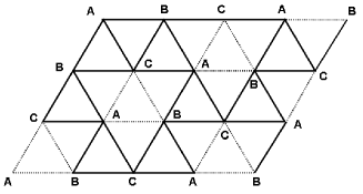
Figure 1: Realization of partial VBS order on a triangular lattice with spin $S=2$. At most four valence bonds can emanate from each site (thick lines), forming a regular array of “missing bonds” (dotted triangles). Magneto-elastic coupling can alter the bond distance depending on the presence/absence of the valence bond. Three inequivalent sites are denoted A, B, and C.

Our ideas are illustrated in Fig. 1 for $S=2$ and $z=6$ (triangular lattice). Such states are energetically unfavorable in comparison to the magnetically ordered state which makes use of the exchange energy for all six neighbors. On the other hand, the spin-lattice coupling can reduce the distance for a pair of sites forming a valence bond, and increase it for sites lacking a bond. The gain in the exchange energy achieved in this way will overcome the loss from the two missing bonds for a sufficiently large coupling strength, and the VBS state is energetically favored over the magnetically ordered state.

We provide a quantitative justification of our claim by analyzing the lattice-coupled spin Hamiltonian,

$$H=\sum_{\langle ij\rangle}J_{ij}S_{i}\cdot S_{j}+{\frac{K}{2}}\sum_{i}u_{i}^{2},$$ (1)

taking $J_{ij}=J_{0}(d^{0}_{ij}/d_{ij})^{\gamma}$ with the equilibrium and actual ionic separations given by $d_{ij}^{0}$ and $d_{ij}$, respectively. For transition metal ions $\gamma$ is a rather large number, ranging between 6-14harrison . Displacement of the $i$-th site is given by $u_{i}$, which costs an elastic energy of $(K/2)u_{i}^{2}$. For ease of analysis, we Taylor-expand $J_{ij}$ in small displacements as $J_{ij}=J_{0}[1-\gamma\hat{e}_{ji}\cdot(u_{j}-u_{i})]$, taking $d^{0}_{ij}=1$, and $\hat{e}_{ji}=(r_{j}-r_{i})/|r_{j}-r_{i}|$ is the unit vector connecting the equilibrium ionic sites, $r_{i}$ and $r_{j}$.

In the following we re-define $u_{i}\rightarrow u_{i}/\sqrt{K}$ and absorb $\gamma/\sqrt{K}$ as $\alpha$, while the overall energy scale $J_{0}$ is normalized to one. Because of the large value of $\gamma$, a small displacement can lead to a substantial difference in the exchange energy. Only the adiabatic limit of the phonon dynamics is considered as we are ignoring the kinetic energy. The model is defined for the two-dimensional triangular lattice with the nearest-neighbor exchange interaction $\langle ij\rangle$ only. A similar model on a linear chain and on a square lattice has been studied earliermila . We look for the ground state of the above Hamiltonian within the Schwinger boson mean-field theory (SBMFT)AA .

One re-writes the above Hamiltonian using a pair of Schwinger bosons $(b_{i1},b_{i2})$ defined at each site,

$$S_{i}\cdot S_{j}\rightarrow-{\frac{1}{2}}A^{+}_{ij}A_{ij},$$ (2)

where $A_{ij}=b_{i1}b_{j2}-b_{i2}b_{j1}$, and decouple it by introducing the order parameter $Q_{ij}=\langle A_{ij}\rangle=-Q_{ji}$. Non-zero $|Q_{ij}|$ implies finite amplitude of a singlet bond for the $\langle ij\rangle$ link. The resulting mean-field Hamiltonian is

$$H_{MF} = -{\frac{1}{2}}\sum_{i}\sum_{j\in i}\overline{\Delta}_{ij}b_{i1}b_{j2}-{\frac{1}{2}}\sum_{i}\sum_{j\in i}\Delta_{ij}b^{+}_{j2}b^{+}_{i1}$$ (3)

$$+\sum_{i}\lambda_{i}(b^{+}_{i1}b_{i1}+b^{+}_{i2}b_{i2}-2S)+{\frac{1}{2}}\sum_{i}u_{i}^{2},$$

where we have introduced $\Delta_{ij}\equiv J_{ij}Q_{ij}$, and $j\in i$ to indicate all nearest neighbors of $i$. Lagrange multipliers $\lambda_{i}$ are fixed by the constraint that $\partial\langle H_{MF}\rangle/\partial\lambda_{i}=0$ which also amounts to requiring $\langle b^{+}_{i1}b_{i1}+b^{+}_{i2}b_{i2}\rangle=2S$ at each site. Energy minimization requires that $u_{i}$ obeysjia ; mila

$$u_{i}=\alpha\sum_{j\in i}\hat{e}_{ij}\langle S_{i}\cdot S_{j}\rangle=-{\frac{\alpha}{2}}\sum_{j\in i}\hat{e}_{ij}|Q_{ij}|^{2}.$$ (4)

We proceed to solve the mean-field Hamiltonian assuming (i) homogeneous pairing and (ii) inhomogeneous pairing of the type described in Fig. 1, and compare their energies.

For the homogeneous case, the singlet pair amplitudes are taken as $Q_{i,i+e_{1}}=Q_{i,i+e_{2}}=Q_{i,i+e_{3}}=iQ$ and $\lambda_{i}=\lambda$. The three unit vectors are defined by $\hat{e}_{1}=(1,0)$, $\hat{e}_{2}=(-1/2,\sqrt{3}/2)$, $\hat{e}_{3}=(-1/2,-\sqrt{3}/2)$. Passing to momentum space, the Hamiltonian becomes

$$H_{MF}=\sum_{k}(\begin{array}[]{cc}b^{+}_{k1}&b_{-k2}\end{array})\left(\begin{array}[]{cc}\lambda&\Delta_{k}\\ \Delta_{k}&\lambda\end{array}\right)\left(\begin{array}[]{c}b_{k1}\\ b^{+}_{-k2}\end{array}\right),$$ (5)

where $\Delta_{k}=Q\sum_{\alpha=1}^{3}\sin(k\cdot\hat{e}_{\alpha})$. The equation of motion for the boson operators can be derived from Eq. (5) and utilizing the boson commutation algebra,

$$E_{k}\left(\begin{array}[]{c}u_{k}\\ v_{k}\end{array}\right)=\left(\begin{array}[]{cc}\lambda&\Delta_{k}\\ -\Delta_{k}&-\lambda\end{array}\right)\left(\begin{array}[]{c}u_{k}\\ v_{k}\end{array}\right),$$ (6)

which has a pair of eigenvalues $\pm E_{k}$, $E_{k}=\sqrt{\lambda^{2}-\Delta_{k}^{2}}$. Boson occupation numbers $n_{i}=\langle b_{i1}^{+}b_{i1}+b_{i2}^{+}b_{i2}\rangle$, and the pairing amplitudes are worked out

$$n_{i}+1={\frac{1}{N_{k}}}\sum_{k}{\frac{\lambda}{E_{k}}}=2S+1,$$

$$Q={\frac{1}{3N_{k}}}\sum_{k}\sum_{\alpha=1}^{3}{\frac{\Delta_{k}}{E_{k}}}\sin(k\cdot e_{\alpha}).$$ (7)

The $k$-sum is restricted to the first Brillouin zone of the triangular lattice, and $N_{k}$ are the number of distinct $k$-points. Upon solving Eq. (7) we obtain $Q=\sqrt{3}S+0.1161$ and the ground-state energy per site

$$E^{h}_{g.s.}=-{\frac{3}{2}}Q^{2}=-{\frac{3}{2}}(\sqrt{3}S+0.1161)^{2}.$$ (8)

There is no energy gain from magneto-elastic coupling since lattice displacement is zero for the uniform bond amplitudes.

Next, we consider the situation where two distinct bond amplitudes, $Q_{1}$ and $Q_{2}$, corresponding to dotted and thick lines in Fig. 1, exist. Non-zero lattice displacement develops with magnitude $|u_{i}|=(\sqrt{3}\alpha/2)(Q_{2}^{2}-Q_{1}^{2})$, and the directions consistent with the uniform expansion of those triangles in Fig. 1 lacking a valence bond. Exchange energy $J_{ij}$ is similarly modulated, $J_{1}=1-(3\alpha^{2}/2)(Q_{2}^{2}-Q_{1}^{2})$, $J_{2}=1+(3\alpha^{2}/4)(Q_{2}^{2}-Q_{1}^{2})$, and finally, $\Delta_{1}=J_{1}Q_{1}$ and $\Delta_{2}=J_{2}Q_{2}$.

Corresponding equation of motion of the operators can be worked out. Six-dimensional eigenvectors $\psi_{k}=(u_{Ak}~{}u_{Bk}~{}u_{Ck}~{}v_{Ak}~{}v_{Bk}~{}v_{Ck})^{T}$ satisfy an equation of motion $E_{k}\psi_{k}=M_{k}\psi_{k}$ where

$$M_{k}=\left(\begin{array}[]{cccccc}\lambda&0&0&0&-i\eta_{1k}&i\overline{\eta}_{3k}\\ 0&\lambda&0&i\overline{\eta}_{1k}&0&-i\eta_{2k}\\ 0&0&\lambda&-i\eta_{3k}&i\overline{\eta}_{2k}&0\\ 0&i\eta_{1k}&-i\overline{\eta}_{3k}&-\lambda&0&0\\ -i\overline{\eta}_{1k}&0&i\eta_{2k}&0&-\lambda&0\\ i\eta_{3k}&-i\overline{\eta}_{2k}&0&0&0&-\lambda\end{array}\right),$$ (9)

and

$$2\eta_{1k} = \Delta_{1}e^{ik\cdot e_{1}}+\Delta_{2}e^{ik\cdot e_{2}}+\Delta_{2}e^{ik\cdot e_{3}}$$

$$2\eta_{2k} = \Delta_{2}e^{ik\cdot e_{1}}+\Delta_{1}e^{ik\cdot e_{2}}+\Delta_{2}e^{ik\cdot e_{3}}$$

$$2\eta_{3k} = \Delta_{2}e^{ik\cdot e_{1}}+\Delta_{2}e^{ik\cdot e_{2}}+\Delta_{1}e^{ik\cdot e_{3}}.$$ (10)

Each eigenvector is normalized to obey $|u_{Ak}|^{2}+|u_{Bk}|^{2}+|u_{Ck}|^{2}-|v_{Ak}|^{2}-|v_{Bk}|^{2}-|v_{Ck}|^{2}=1$.

While the problem is not tractable analytically, it can be shown that the (extreme) limit of $\Delta_{1}=0$ yields an analytical answer. We call it the “kagome limit”, where the non-zero $\Delta$’s form a network topologically equivalent to the kagome lattice. Using the linear Taylor expansion of exchange energy $J_{1}$ and $J_{2}$, the ground state energy is given by

$$E^{m}_{g.s.}=-{1\over 2}Q_{1}^{2}-Q_{2}^{2}-{3\over 8}\alpha^{2}(Q_{2}^{2}-Q_{1}^{2})^{2},$$ (11)

for the lattice-distorted situation. In the kagome limit the self-consistency equations give $Q_{1}=\sqrt{3}S-0.2128$, and $Q_{2}=\sqrt{3}S+0.1823$. Finally, in order to make $J_{1}=0$, $\alpha$ must be equal to $0.4946$. In comparing Eq. (8) with Eq. (11) with $S=2$, the state with modulated bond is found to have a lower energy.

The stability of the bond-modulated state can be argued on a more general basis. Restoring the various energy scales, the ground state energies of homogeneous and modulated bonds are given by

$$E^{h}_{g.s.}=-{3\over 2}J_{0}Q^{2},~{}~{}E^{m}_{g.s.}=-{1\over 2}J_{1}Q_{1}^{2}-J_{2}Q_{2}^{2}+{K\over 2}u^{2}.$$ (12)

As our analysis in the kagome limit showed, $Q$ depends slowly on the amount of distortion $u$, and all three $Q$ values are given by $Q\approx Q_{1}\approx Q_{2}\approx\sqrt{3}S$. Much more dramatic dependence on $u$ arises from $J_{1}$ and $J_{2}$, which reads $J_{1}=J_{0}/(1+\sqrt{3}u)^{\gamma}$ and $J_{2}=J_{0}/(1-\sqrt{3}u/2)^{\gamma}$ assuming small $u$. Using $Q=Q_{1}=Q_{2}=\sqrt{3}S=2\sqrt{3}$, the energy difference $E^{h}_{g.s.}-E^{m}_{g.s.}$ is shown to be a monotone decreasing function of $u$ for $K/J_{0}\leq 27\gamma(\gamma+1)$, indicating a lattice instability. The quartic term in the potential energy for $u$ not included in Eq. (1) will restore the stability at a finite $u$ and favor the lattice reconstruction indicated in Fig. 1.

The mean-field ground state features Bose condensation for both uniform and non-uniform states which are the hallmarks of magnetic order. For $k=k^{*}$ at which the Bose condensation occurs, the ground state is described by a form $|\mathrm{LRO}\rangle=(\gamma^{+}_{k^{*}})^{N_{k^{*}}}|0\rangle$ ($N_{k^{*}}$ = number of bosons in the condensed state). For other $k$ values the ground state is defined by $\gamma_{k}|\mathrm{MF}\rangle=0$, where $\gamma_{k}$ are the quasiparticle operators diagonalizing the mean-field Hamiltonian, Eq. (3). The uncondensed part, written in real space, is of the general form, $|\mathrm{MF}\rangle=\exp\left\{{\frac{1}{2}}\sum_{ij}u_{ij}(b^{+}_{i1}b^{+}_{j2}-b^{+}_{j1}b^{+}_{i2})\right\}|0\rangle,$ representing a gapped spin liquidAA ; Book . The sensitivity of the ground state on a particular spin quantum number $S$ arises when we make a projection to a fixed $S$: $|\mathrm{VBS}\rangle=P_{S}|\mathrm{MF}\rangle$. The full ground state is a direct product of the condensed and the uncondensed parts, $|\mathrm{GS}\rangle=|\mathrm{LRO}\rangle\otimes|\mathrm{VBS}\rangle$.

With $S=2$, the projected ground state consists of a large number of valence bond configurations all sharing the property that each site has four valence bonds emanating form it. Among those states, the VBS state depicted in Fig. 1 is the one most consistent with the kagome limit. Such a state, in turn, is described by the AKLT state:

$$|\mathrm{AKLT}\rangle=\prod_{\langle ij\rangle^{\prime}}(b_{i1}^{+}b_{j2}^{+}-b_{i2}^{+}b_{j1}^{+})|0\rangle.$$ (13)

$\langle ij\rangle^{\prime}$ runs over the four valence bonds depicted in Fig. 1.

Although the equivalence of $|\mathrm{AKLT}\rangle$ with $|\mathrm{VBS}\rangle_{S=2}$ cannot be established rigorously, it is still reasonable to expect that the physical properties embodied in the $|\mathrm{AKLT}\rangle$ state will reflect those of the $|\mathrm{VBS}\rangle_{S=2}$ Raykin .

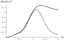
Figure 2: Static structure factor ${\cal S}(k)=\langle S_{-k}\cdot S_{k}\rangle$ for the $|\mathrm{AKLT}\rangle$ state in Eq. (13). Solid line is ${\cal S}(k,0)$, and the dashed line is ${\cal S}(0,k)$. MC calculations were performed on $N=90\times 90$ punctured triangular lattice.

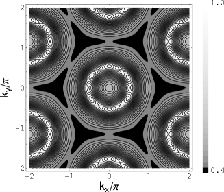
Figure 3: Contour of the energy spectrum for (a) VBS state given in Eq. (13), and (b) spin waves in triangular lattice. Both plots are scaled by $6J$. (c) Disperson along $(k,0)$ direction for VBS (solid) and spin wave (dashed).

The quasiparticle spectrum obtained from diagonalizing Eq. (9) reduces to the familiar spin wave modesmattson . The excitation energies for the AKLT ground state given above can be worked out in a manner parallel to the calculation for the gapped spin liquid in one-dimensional, $S=1$ chainAAH . We adopt the method of single mode approximation (SMA), and write the excitation energy $\Delta(k)$:

$$\Delta(k)=\frac{\langle[S_{-k}\cdot,[H,S_{k}]\rangle}{2\langle S_{-k}\cdot S_{k}\rangle}$$

$$=2z^{\prime}B_{1}\times{\frac{1-(1/3)\sum_{\alpha=1}^{3}\cos[k\cdot e_{\alpha}]}{(1/N)\sum_{i,j}\langle S_{i}\cdot S_{j}\rangle e^{ik\cdot(r_{j}-r_{i})}}}.$$ (14)

The averages $\langle\cdots\rangle$ are to be taken with respect to $|\mathrm{AKLT}\rangle$ state given in Eq. (13). The nearest-neighbor spin-spin correlation $-B_{1}$, as well as all other averages $\langle S_{i}\cdot S_{j}\rangle$ can be evaluated using the standard Monte Carlo (MC) methodBook ; MC . The effective coordination number on the kagome lattice is $z^{\prime}=4$; the number of sites of the triangular lattice is $N$.

The structure factor ${\cal S}(k)\equiv\langle S_{-k}\cdot S_{k}\rangle$ vanishes in the $k=0$ limit due to the singlet character of the AKLT state. The next term in the small-$k$ expansion gives ${\cal S}(k)\approx\Gamma k^{2}$, where $-\Gamma=(1/N)\sum_{i,j}(r_{j}-r_{i})^{2}\langle S_{i}\cdot S_{j}\rangle$. The numerator in Eq. (14) also vanishes as $k^{2}$, giving the $k=0$ gap of magnitude $\Delta(k=0)=8J\times(B_{1}/\Gamma)$.

The AKLT state has only short-range order as manifested by an exponential decay of the spin-spin correlation, $|\langle S_{i}\cdot S_{j}\rangle|\sim e^{-1.467|i-j|}$, in our MC simulation. In Fig. 2 we present results for the static structure factor. The $k=0$ gap obtained from ${\cal S}(k)$ is $\Delta(0)\simeq 0.5\times(6J)$.

Figure 3 displays excitation spectrum $\Delta(k)$ for $|\mathrm{VBS}\rangle$ according to Eq. (14), and the standard spin wave in the uniform $|\mathrm{LRO}\rangle$. The new spectrum $\Delta(k)$ is characterized by a broad minimum (dark region) that exist around the zone boundary of the Brillouin zone, and in principle should be observable in the neutron scattering. The spin waves and the new excitation mode we find reflect the two kinds of broke symmetries found in the ground state. Interaction between the two modes should exist, which requires going beyond the quadratic Hamiltonian (3) to include fluctuation terms.

In summary, we propose that a VBS state can be stabilized in two-dimensional antiferromagnetic spins with a mismatch of $2S$ and $z$, when a sufficiently strong coupling to the lattice deformation exists. As an example, we analyze $S=2$, $z=6$ (triangular) model in the Schwinger boson mean-field theory and show that the energy is lower for the lattice-deformed state. Corresponding gapped spin excitation energies are calculated within the single-mode approximation.