Perturbation theory for optical excitations in the one-dimensional extended Peierls–Hubbard model

Abstract

For the one-dimensional, extended Peierls–Hubbard model we calculate analytically the ground-state energy and the single-particle gap to second order in the Coulomb interaction for a given lattice dimerization. The comparison with numerically exact data from the Density-Matrix Renormalization Group shows that the ground-state energy is quantitatively reliable for Coulomb parameters as large as the band width. The single-particle gap can almost triple from its bare Peierls value before substantial deviations appear. For the calculation of the dominant optical excitations, we follow two approaches. In Wannier theory, we perturb the Wannier exciton states to second order. In two-step perturbation theory, similar in spirit to the GW-BSE approach, we form excitons from dressed electron-hole excitations. We find the Wannier approach to be superior to the two-step perturbation theory. For singlet excitons, Wannier theory is applicable up to Coulomb parameters as large as half band width. For triplet excitons, second-order perturbation theory quickly fails completely.

1 Introduction

Electrons in low-dimensional systems behave very differently from their three-dimensional counterparts. On the one hand, at low temperatures they tend to distort the lattice (Peierls effect [1]). For example, poly-acetylene as the simplest $\pi$-conjugated polymer shows an alternation between short and long bonds [2]. At the Peierls transition a gap opens in the single-particle spectrum and the metal turns into a Peierls insulator. On the other hand, the electron-electron interaction provides a relevant perturbation in one dimension. For example, metals in one dimension are Luttinger liquids in which the low-energy charge and spin excitations propagate with different velocities so that quasi-particles as in Landau Fermi-Liquid Theory are absent in the single-particle spectral function [3, 4]. At commensurate band fillings, the electron-electron interaction induces Umklapp scatterings which turn the metal state into a Mott insulator.

This immediately raises the question: which of the two perturbations, Peierls distortion or Mott transition, dominates the other one? This question can be answered within the framework of field theory because both the electron-lattice and the electron-electron interactions destroy the metallic phase even in the limit of weak coupling. As has been shown in [5, 6], the Peierls distortion is always a relevant perturbation in the sense of a renormalization-group analysis whereas the Umklapp scatterings which cause the Mott transition are only marginally relevant. At large Coulomb interactions when the system is a Mott insulator, the Peierls distortion is also present at low temperatures because the effective spin system undergoes a spin-Peierls transition. Therefore, one-dimensional lattices are expected to be Peierls distorted at zero temperature, irrespective of the presence of the electron-electron interaction.

In presence of a Peierls distortion and one electron per lattice site (half band-filling), the Peierls insulator can be described in terms of a filled lower Peierls band and an empty upper Peierls band which are separated by a finite Peierls gap whose size is proportional to the dimerization strength. In principle, the finite Peierls gap permits a perturbative treatment of the electron-electron interaction. It should be clear, however, that such a perturbative treatment is limited to ‘weak coupling’, and the range of the validity of perturbation theory remains to be determined. In particular, even the screened electron-electron interaction in polymers is quite sizable [7], and it remains to be studied in how far Wannier theory and similar perturbative approaches [8, 9] lead to a reliable description of optical excitations in these materials.

In this work, we investigate the extended Peierls–Hubbard model at half band-filling which models the Peierls distortion and the Coulomb interaction in ideal poly-acetylene. The model is introduced in section 2. In section 3 we use standard Rayleigh-Schrödinger perturbation theory to calculate the ground-state energy to second order in the Coulomb interaction and compare our results to numerically exact data from the Density-Matrix Renormalization Group (DMRG). We show that second-order perturbation theory is applicable up to interaction strengths as large as the band width. In section 4 we observe the same behavior for the gap for single-particle excitations which increases quickly as a function of the interaction strength.

In order to study optical excitations, we follow two routes because Rayleigh–Schrödinger perturbation theory is inapplicable for a description of bound electron-hole pairs. In section 5 we develop Wannier perturbation theory to second order where an exciton is formed already in first order. Alternatively, we introduce the ‘two-step perturbation theory’ in which the exciton is formed in a second step after the electrons and holes have been dressed first. In section 6 the comparison of our analytical results with those from the DMRG show that second-order Wannier theory is superior to the two-step perturbation theory. The singlet exciton is reasonably well described by Wannier theory for moderate interactions but perturbation theory quickly fails for the triplet exciton. We close our presentation with concluding remarks in section 7. Technical details of the calculations are deferred to the appendix.

2 Hamilton Operator

2.1 Peierls Model

We investigate spin-1/2 electrons on a periodically distorted chain of $L$ sites whose motion is described by the Peierls Hamiltonian,

$$\hat{T}=(-t)\sum_{l;\sigma}\left(1+(-1)^{l}\delta\right)\left(\hat{c}_{l,\sigma}^{+}\hat{c}_{l+1,\sigma}^{\phantom{+}}+\hat{c}_{l+1,\sigma}^{+}\hat{c}_{l,\sigma}^{\phantom{+}}\right)\;,$$ (1)

where $\hat{c}^{+}_{l,\sigma}$, $\hat{c}_{l,\sigma}$ are creation and annihilation operators for electrons with spin $\sigma=\uparrow,\downarrow$ on site $l$. The lattice spacing is set to unity, $a_{0}\equiv 1$. Since we are interested in the insulating phase, we consider exclusively a half-filled band where the number of electrons $N=2N_{\sigma}$ equals the number of lattice sites $L$. For our analytical calculations, we choose periodic boundary conditions and $L/2$ even. For the DMRG investigations, open boundary conditions are employed.

The Peierls operator is diagonal in momentum space [10],

$$\hat{T}=\sum_{k;\sigma}E(k)\left(\hat{b}^{+}_{k,\sigma}\hat{b}_{k,\sigma}^{\phantom{+}}-\hat{a}^{+}_{k,\sigma}\hat{a}_{k,\sigma}^{\phantom{+}}\right)\;,$$ (2)

where $k=2\pi m/L$, $m=-L/2,\ldots,L/2-1$, are the momenta from the reduced Brillouin zone. The dispersion relation for the upper and lower Peierls bands is

$$E(k)=\sqrt{\epsilon(k)^{2}+\Delta(k)^{2}}$$ (3)

with

$$\epsilon(k) = -2t\cos(k)\;,$$ (4)

$$\Delta(k) = 2t\delta\sin(k)\;.$$

The Fermi operators for the electrons in the Peierls bands obey

$$\hat{a}_{k,\sigma} \equiv\alpha_{k}\hat{c}_{k,\sigma}+{\rm i}\beta_{k}\hat{c}_{k+\pi,\sigma}\;,$$

$$\hat{b}_{k,\sigma} \equiv\beta_{k}\hat{c}_{k,\sigma}-{\rm i}\alpha_{k}\hat{c}_{k+\pi,\sigma}$$ (5)

with

$$\alpha_{k} = \sqrt{\frac{1}{2}\left(1-\frac{\epsilon(k)}{E(k)}\right)}\;,$$

$$\beta_{k} = {\rm sgn}[\Delta(k)]\sqrt{\frac{1}{2}\left(1+\frac{\epsilon(k)}{E(k)}\right)}\;,$$ (6)

and ${\rm sgn}(x\neq 0)=x/|x|$ is the sign function. For the inverse transformation and other useful relations, see A.

2.2 Coulomb interaction

The electrons are supposed to interact locally with strength $U$. The Hubbard interaction reads

$$\hat{U}=U\sum_{l}(\hat{n}_{l,\uparrow}-1/2)(\hat{n}_{l,\downarrow}-1/2)\;,$$ (7)

where $\hat{n}_{l,\sigma}=\hat{c}^{+}_{l,\sigma}\hat{c}_{l,\sigma}^{\phantom{+}}$ is the local density operator at site $l$ for spin $\sigma$. Screening is not very efficient in an insulator. Therefore, we take into account the long-range Coulomb interaction of the electrons in the form of a $1/r$ potential of effective strength $V$,

$$\hat{V}=\sum_{r}V(r)\sum_{l}\left(\hat{n}_{l}-1\right)\left(\hat{n}_{l+r}-1\right)\;,$$ (8)

where $\hat{n}_{l}=\hat{n}_{l,\uparrow}+\hat{n}_{l,\downarrow}$ counts the electrons on site $l$ and $V(r)=V/(2r)$ describes the Coulomb potential. For the analytical calculations, the specific form of $V(r)$ is not important.

2.3 Extended Peierls–Hubbard model

Altogether we investigate the one-dimensional extended Peierls–Hubbard model,

$$\hat{H}=\hat{T}+\hat{U}+\hat{V}\equiv\hat{T}+\hat{W}\;.$$ (9)

The Hamiltonian is invariant under SU(2) spin transformations so that the total spin is a good quantum number. Including the charge-SU(2) the Hamiltonian is SO(4) symmetric. Moreover, it exhibits particle-hole symmetry, i.e., $\hat{H}$ is invariant under the transformation

$${\rm PH}:\qquad\hat{c}_{l,\sigma}^{+}\mapsto(-1)^{l}\hat{c}_{l,\sigma}\quad;\quad\hat{c}_{l,\sigma}\mapsto(-1)^{l}\hat{c}_{l,\sigma}^{+}\;.$$ (10)

The chemical potential $\mu=0$ guarantees a half-filled band for all temperatures [11].

The Peierls dimerization ($\delta\neq 0$) and the Coulomb interaction ($U,V\neq 0$) individually lead to an insulating ground state at half band-filling. A field-theoretical investigation shows [5, 6] that the lattice distortion is always a relevant perturbation, i.e., it occurs for all values of the Coulomb interaction. Therefore, the Peierls insulator provides a valid starting point for a perturbation expansion in the Coulomb interaction.

3 Ground-state energy to second order

3.1 Analytical results

For the calculation of the ground-state energy $E_{0}$ we apply standard Rayleigh–Schrödinger perturbation theory to second order,

$$E_{0} = E_{0}^{(0)}+E_{0}^{(1)}+E_{0}^{(2)}\;,$$

$$E_{0}^{(1)} = E_{0}^{U}+E_{0}^{V}\;,$$ (11)

$$E_{0}^{(2)} = E_{0}^{U^{2}}+E_{0}^{V^{2}}+E_{0}^{UV}\;.$$

The expectation value of $\hat{H}$ with the ground state of the Peierls insulator (filled lower Peierls band)

$$|{\rm FS}\rangle=\prod_{k,\sigma}\hat{a}_{k,\sigma}^{+}|{\rm vacuum}\rangle$$ (12)

contributes

$$E_{0}^{(0)} = \langle{\rm FS}|\hat{T}|{\rm FS}\rangle=-2\sum_{k}2t\sqrt{\cos(k)^{2}+\delta^{2}\sin(k)^{2}}\;,$$

$$E_{0}^{U} = \langle{\rm FS}|\hat{U}|{\rm FS}\rangle=0\;,$$ (13)

$$E_{0}^{V} = \langle{\rm FS}|\hat{V}|{\rm FS}\rangle=-L\sum_{-L/2\leq r<L/2\atop{r|2=1}}2V(r)[(A_{\delta}(r))^{2}+(B_{\delta}(r))^{2}]\;,$$ (14)

where ($r|2=1$) denotes all odd $r$, $A_{\delta}(r)$, $B_{\delta}(r)$ are defined in (83), and (88) is used for the derivation of (13). For the Peierls insulator we have in the thermodynamic limit,

$$\lim_{L\to\infty}\frac{E_{0}^{(0)}}{L}=-(4t/\pi){\rm E}(1-\delta^{2})$$ (15)

where ${\rm E}(m)$ is the complete elliptic integral of the second kind.

3.1.1 Second-order excitations.

To second order, particle-hole excitations of the Peierls ground states must be considered. In general, we denote excitations with $r$ ($s$) particle-hole excitations in the $\uparrow$-sector ($\downarrow$-sector) by $|rs\rangle$. Fig. 1 shows two particle-hole excitations with antiparallel spins, i.e., $|11\rangle$, and parallel spins, i.e., $|20\rangle$, respectively. These are all excitations which contribute to the ground-state energy to second order.

Figure 1: Two-particle-hole excitations $|11\rangle$ (top row) and $|20\rangle$ (bottom row).

3.1.2 Second order in the Hubbard interaction.

For the Hubbard interaction, only the states $|11\rangle$ contribute. As input to (11) they give [5]

$$E_{0}^{U^{2}} = \sum_{|11\rangle}\frac{\left|\langle{\rm FS}|\hat{U}|11\rangle\right|^{2}}{E_{0}^{(0)}-E_{|11\rangle}^{(0)}}$$ (16)

$$= -\left(\frac{U}{L}\right)^{2}\sum_{k_{1},k_{2},k_{3},k_{4}}\frac{1}{E(k_{1})+E(k_{2})+E(k_{3})+E(k_{4})}$$

$$\hphantom{-\left(\frac{U}{L}\right)^{2}\sum_{k_{1},k_{2},k_{3},k_{4}}}\Bigl{\{}\delta_{k_{1}-k_{2}+k_{3}-k_{4},0}[u_{1}(k_{1},k_{2},k_{3},k_{4})]^{2}$$

$$\hphantom{-\left(\frac{U}{L}\right)^{2}\sum_{k_{1},k_{2},k_{3},k_{4}}}+\delta_{k_{1}-k_{2}+k_{3}-k_{4},\pm\pi}[u_{2}(k_{1},k_{2},k_{3},k_{4})]^{2}\Bigr{\}}$$

with $u_{1,2}(k_{1},k_{2},k_{3},k_{4})$ from (82).

3.1.3 Second order in the long-range interaction.

The long-range Coulomb interaction also induces scatterings between particles with the same spin. Therefore, we have three contributions to second order. We find [5]

$$E_{0}^{V^{2}|10\rangle}=\sum_{|10\rangle}\frac{\left|\langle{\rm FS}|\hat{V}|10\rangle\right|^{2}}{E_{0}^{(0)}-E_{|10\rangle}^{(0)}}=\sum_{k}\frac{V^{2}v_{0}(k)^{2}}{E(k)}\;,$$ (17)

where $v_{0}(k)$ is given in (84),

$$E_{0}^{V^{2}|11\rangle} = \sum_{k_{1},k_{2},k_{3},k_{4}}\frac{1}{E(k_{1})+E(k_{2})+E(k_{3})+E(k_{4})}$$ (18)

$$\hphantom{\sum_{k_{1},k_{2},k_{3},k_{4}}}\Bigl{\{}\delta_{k_{1}-k_{2}+k_{3}-k_{4},0}[v_{1}(k_{1},k_{2},k_{3},k_{4})]^{2}$$

$$\hphantom{\sum_{k_{1},k_{2},k_{3},k_{4}}}+\delta_{k_{1}-k_{2}+k_{3}-k_{4},\pm\pi}[v_{2}(k_{1},k_{2},k_{3},k_{4})]^{2}\Bigr{\}}$$

with $v_{1,2}(k_{1},k_{2},k_{3},k_{4})$ from (86) and (87), and

$$E_{0}^{V^{2}|20\rangle} = -\left(\frac{V}{L}\right)^{2}\sum_{k_{1}<k_{3},k_{2}<k_{4}}\frac{1}{E(k_{1})+E(k_{2})+E(k_{3})+E(k_{4})}$$

$$\Bigl{[}\delta_{k_{1}-k_{2}+k_{3}-k_{4},0}[v_{1}(k_{1},k_{2},k_{3},k_{4})-v_{1}(k_{1},k_{4},k_{3},k_{2})]^{2}$$

$$+\delta_{k_{1}-k_{2}+k_{3}-k_{4},\pm\pi}[v_{2}(k_{1},k_{2},k_{3},k_{4})-v_{2}(k_{1},k_{4},k_{3},k_{2})]^{2}\Bigr{]}\,.$$

The summation restriction in the last term can be relaxed. Due to the symmetry of the functions $v_{1,2}(k_{1},k_{2},k_{3},k_{4})$ we may multiply the last contribution by a factor $1/4$ and sum over all momenta from the reduced Brillouin zone. Due to the spin-flip symmetry we altogether have

$$E_{0}^{V^{2}}=2E_{0}^{V^{2}|10\rangle}+E_{0}^{V^{2}|11\rangle}+2E_{0}^{V^{2}|20\rangle}$$ (20)

as input to (11).

3.1.4 Second-order mixed interactions.

Only the states $|11\rangle$ contribute to order $UV$,

$$E_{0}^{UV} = \sum_{|11\rangle}\frac{\langle{\rm FS}|\hat{V}|11\rangle\langle 11|\hat{U}|{\rm FS}\rangle+{\rm c.c.}}{E_{0}^{(0)}-E_{|11\rangle}^{(0)}}$$ (21)

$$= \frac{2UV}{L^{2}}\sum_{k_{1},k_{2},k_{3},k_{4}}\frac{1}{E(k_{1})+E(k_{2})+E(k_{3})+E(k_{4})}$$

$$\Bigl{[}\delta_{k_{1}-k_{2}+k_{3}-k_{4},0}u_{1}(k_{1},k_{2},k_{3},k_{4})v_{1}(k_{1},k_{2},k_{3},k_{4})$$

$$+\delta_{k_{1}-k_{2}+k_{3}-k_{4},\pm\pi}u_{2}(k_{1},k_{2},k_{3},k_{4})v_{2}(k_{1},k_{2},k_{3},k_{4})\Bigr{]}\;.$$

3.2 Comparison with numerical results

3.2.1 Finite-size effects.

First, we demonstrate that lattices with $L=100$ provide results which are very close to the thermodynamic limit. Fig. 2 gives an example for $U=2V=2t$ and $\delta=0.2$.

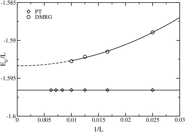
Figure 2: Ground-state energy density $E_{0}/L$ as a function of inverse system size for fixed $U=2V=2t$ and $\delta=0.2$ in the DMRG and perturbation theory; lines are polynomial fits. Note the resolution of the ordinate.

The result from perturbation theory for periodic boundary conditions shows almost no size dependence whereas the data from the numerical density-matrix renormalization group displays the typical parabolic convergence in $1/L$. The comparison shows that the results for $L=100$ are almost identical to the result in the thermodynamic limit. In particular, the differences between perturbation theory and the numerically exact DMRG are small but significant. The same observation holds equally well for other choices of (finite) model parameters $U,V,\delta$.

In the following we shall show results for $L=100$ and take them as representative for the thermodynamic limit.

3.2.2 Fixed ratio $U/V$.

Next, we discuss the ground-state energy density as a function of the Coulomb interaction for a fixed ratio of $U/V$. This is shown in Fig. 3 where we compare the DMRG data with the results from first and second-order perturbation theory. It is seen that the second-order correction considerably improves the agreement between the numerically exact DMRG data and perturbation theory.

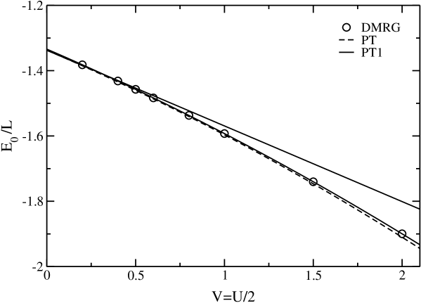
Figure 3: Ground-state energy density $E_{0}/L$ as a function of $V$ for fixed $U/V=2$, $L=100$, and $\delta=0.2$ in the DMRG (circles) and perturbation theory. Lines are polynomial fits. For $U=V=0$, $\lim_{L\to\infty}E_{0}^{(0)}/L\approx 1.34$.

3.2.3 Fixed $V$.

In general, the influence of the Hubbard interaction is well described by the second-order term, as can be seen from Fig. 4. It shows that perturbation theory works very well even when $U$ is as large as the band width $W=4t$. The agreement is even better for smaller $V$.

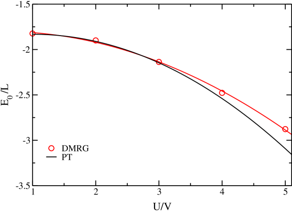
Figure 4: Ground-state energy density $E_{0}/L$ as a function of $U$ for $V=2t$, $L=100$, and $\delta=0.2$ in the DMRG (circles) and perturbation theory. Lines are polynomial fits.

3.2.4 Conclusion.

The above comparison has been made for a sizable value of the Peierls dimerization, $\delta=0.2$, so that the bare Peierls gap, $\Delta^{\rm P}=4t\delta=0.8t$, is substantial. Naturally, the comparison between the DMRG and second-order perturbation theory becomes less favorable when we decrease $\delta$ to realistic values, $\delta<0.1$; see section 7. Nevertheless, even for small values of $\delta$, the formulae in this section give a very good estimate for the ground-state energy density for a large range of Coulomb interactions, $U\approx 2V\leq W$.

4 Single-particle gap to second order

In order to generate current-carrying excitations in a Peierls–Mott insulator, the gap for single-particle excitations must be overcome. It is defined by

$$\Delta_{1}=[E_{0}(L+1)-E_{0}(L)]-[E_{0}(L)-E_{0}(L-1)]\;,$$ (22)

where $E_{0}(N)$ is the ground-state energy of the system with $N$ electrons. Due to particle-hole symmetry we have

$$\Delta_{1}=2[E_{0}(L+1)-E_{0}(L)]\;.$$ (23)

4.1 Analytical results

For the perturbative calculation of the single-particle gap $\Delta_{1}$ we apply standard Rayleigh–Schrödinger perturbation theory again and write

$$\Delta_{1}=\Delta_{1}^{(0)}+\Delta_{1}^{U}+\Delta_{1}^{V}+\Delta_{1}^{U^{2}}+\Delta_{1}^{V^{2}}+\Delta_{1}^{UV}\;.$$ (24)

For the Peierls insulator the first two contributions are readily calculated because the ground state with $N=L+1$ particles is

$$|p\rangle\equiv\hat{b}_{p,\uparrow}^{+}|{\rm FS}\rangle\quad,\quad p=-\pi/2\;,$$ (25)

and, thus,

$$\Delta_{1}^{(0)}=2\left[\langle p|\hat{T}|p\rangle-\langle{\rm FS}|\hat{T}|{\rm FS}\rangle\right]=2E(p)=4t\delta\equiv\Delta^{\rm P}$$ (26)

is the Peierls gap for all system sizes. Due to the spin symmetry we were allowed to use $\sigma=\uparrow$. Moreover, the first-order contributions read

$$\Delta_{1}^{U} = 2\left[\langle p|\hat{U}|p\rangle-\langle{\rm FS}|\hat{U}|{\rm FS}\rangle\right]=0\;,$$ (27)

$$\Delta_{1}^{V} = 2\left[\langle p|\hat{V}|p\rangle-\langle{\rm FS}|\hat{V}|{\rm FS}\rangle\right]$$ (28)

$$= 2\sum_{-L/2<r<L/2\atop{r|2=1}}4tV(r)\frac{\cos(p)\cos(pr)A_{\delta}(r)+\delta\sin(p)\sin(pr)B_{\delta}(r)}{E(p)}$$

$$= \sum_{-L/2<r<L/2\atop{r|2=1}}4V(r)(-1)^{[(r-1)/2]}B_{\delta}(r)\;,$$

where $p=-\pi/2$ was used in the last step.

4.1.1 Second order in the Hubbard interaction.

In the intermediate states an additional $\uparrow$ electron and $r$ ($s$) electron-holes excitations in the $\uparrow$-sector ($\downarrow$-sector) are possible, denoted as $|k;rs\rangle$. There are two contributions to second order in the Hubbard interaction,

$$\Delta_{1}^{U^{2}|01\rangle} = 2\sum_{k_{1},k_{2},k_{3}}\frac{|\langle p|\hat{U}\hat{b}_{k_{1},\downarrow}^{+}\hat{a}_{k_{2},\downarrow}|k_{3}\rangle|^{2}}{E(p)-(E(k_{1})+E(k_{2})+E(k_{3}))}$$ (29)

$$= \left(\frac{U}{L}\right)^{2}\sum_{k_{1},k_{2},k_{3}}\frac{2\left(1-\delta_{p,k_{1}}\right)}{E(p)-(E(k_{1})+E(k_{2})+E(k_{3}))}$$

$$\hphantom{\left(\frac{U}{L}\right)^{2}\sum_{k_{1},k_{2},k_{3}}}\Bigl{[}\delta_{k_{1}-k_{2}+k_{3}-p,0}[u_{2}(k_{1},k_{2},k_{3},p)]^{2}$$

$$\hphantom{\left(\frac{U}{L}\right)^{2}\sum_{k_{1},k_{2},k_{3}}}+\delta_{k_{1}-k_{2}+k_{3}-p,\pm\pi}[u_{1}(k_{1},k_{2},k_{3},p)]^{2}\Bigr{]}\;,$$

and

$$\frac{\Delta_{1}^{U^{2}|11\rangle}}{2} = \sum_{k_{1},k_{2},k_{3},k_{4}}\frac{|\langle p|\hat{U}\hat{b}_{k_{1},\uparrow}^{+}\hat{a}_{k_{2},\uparrow}\hat{b}_{k_{3},\downarrow}^{+}\hat{a}_{k_{4},\downarrow}|p\rangle|^{2}}{-\left(E(k_{1})+E(k_{2})+E(k_{3})+E(k_{4})\right)}-E_{0}^{U^{2}|11\rangle}$$

$$= \left(\frac{U}{L}\right)^{2}\sum_{k_{1},k_{2},k_{3},k_{4}}\frac{\delta_{p,k_{1}}}{E(k_{1})+E(k_{2})+E(k_{3})+E(k_{4})}$$

$$\hphantom{\left(\frac{U}{L}\right)^{2}\sum_{k_{1},k_{2},k_{3},k_{4}}}\Bigl{[}\delta_{k_{1}-k_{2}+k_{3}-k_{4},0}[u_{1}(k_{1},k_{2},k_{3},k_{4})]^{2}$$

$$\hphantom{\left(\frac{U}{L}\right)^{2}\sum_{k_{1},k_{2},k_{3},k_{4}}}+\delta_{k_{1}-k_{2}+k_{3}-k_{4},\pm\pi}[u_{2}(k_{1},k_{2},k_{3},k_{4})]^{2}\Bigr{]}\;.$$

We thus find from these two equations

$$\Delta_{1}^{U^{2}}=\Delta_{1}^{U^{2}|01\rangle}+\Delta_{1}^{U^{2}|11\rangle}$$ (31)

as input to (24).

4.1.2 Second order in the long-range interaction.

To second order in the long-range interaction, the states $|k;10\rangle$ and $|k;01\rangle$ contribute. Note that the fermionic nature of the operators must be taken into account properly, e.g., $\hat{b}_{k,\uparrow}^{+}|p\rangle\equiv-\hat{b}_{p,\uparrow}^{+}|k\rangle$. This gives the contributions

$$\Delta_{1}^{V^{2}|10\rangle} = \sum_{k_{2},k_{1}>k_{3}}\frac{2|\langle p|\hat{V}\hat{b}_{k_{1},\uparrow}^{+}\hat{a}_{k_{2},\uparrow}|k_{3}\rangle|^{2}}{E(p)-(E(k_{1})+E(k_{2})+E(k_{3}))}-2E_{0}^{V^{2}|10\rangle}$$ (32)

$$= \left(\frac{V}{L}\right)^{2}\sum_{k_{2},k_{1}>k_{3}}\frac{2}{E(p)-(E(k_{1})+E(k_{2})+E(k_{3}))}$$

$$\biggl{[}\delta_{k_{1}-k_{2}+k_{3}-p,0}\Bigl{\{}\delta_{p,k_{3}}\delta_{k_{1},k_{2}}Lv_{0}(k_{1})-\delta_{p,k_{1}}\delta_{k_{2},k_{3}}Lv_{0}(k_{3})$$

$$\hphantom{\biggl{[}\delta_{k_{1}-k_{2}+k_{3}-p,0}\Bigl{\{}}+v_{2}(k_{3},p,k_{1},k_{2})-v_{2}(k_{1},p,k_{3},k_{2})\Bigr{\}}^{2}$$

$$\hphantom{\biggl{[}}+\delta_{k_{1}-k_{2}+k_{3}-p,\pm\pi}\Bigl{\{}v_{1}(k_{3},p,k_{1},k_{2})-v_{1}(k_{1},p,k_{3},k_{2})\Bigr{\}}^{2}\biggr{]}$$

$$-2E_{0}^{V^{2}|10\rangle}\;,$$

and

$$\frac{\Delta_{1}^{V^{2}|01\rangle}}{2} = \sum_{k_{1},k_{2},k_{3}}\frac{|\langle p|\hat{V}\hat{b}_{k_{1},\downarrow}^{+}\hat{a}_{k_{2},\downarrow}|k_{3}\rangle|^{2}}{E(p)-(E(k_{1})+E(k_{2})+E(k_{3}))}-E_{0}^{V^{2}|01\rangle}$$ (33)

$$= \left(\frac{V}{L}\right)^{2}\sum_{k_{1},k_{2},k_{3}}\frac{1}{E(p)-(E(k_{1})+E(k_{2})+E(k_{3}))}$$

$$\Bigl{[}\delta_{k_{1}-k_{2}+k_{3}-p,0}\Bigl{\{}\delta_{p,k_{3}}\delta_{k_{1},k_{2}}Lv_{0}(k_{1})+v_{2}(k_{3},p,k_{1},k_{2})\Bigr{\}}^{2}$$

$$+\delta_{k_{1}-k_{2}+k_{3}-p,\pm\pi}\Bigl{\{}v_{1}(k_{3},p,k_{1},k_{2})\Bigr{\}}^{2}\Bigr{]}$$

$$-E_{0}^{V^{2}|01\rangle}\;.$$

Moreover, the states with two particle-hole excitations, $|p;11\rangle$, contribute. We find

$$\frac{\Delta_{1}^{V^{2}|11\rangle}}{2} = \sum_{k_{1},k_{2},k_{3},k_{4}}\frac{|\langle p|\hat{V}\hat{b}_{k_{1},\uparrow}^{+}\hat{a}_{k_{2},\uparrow}\hat{b}_{k_{3},\downarrow}^{+}\hat{a}_{k_{4},\downarrow}|p\rangle|^{2}}{-\left(E(k_{1})+E(k_{2})+E(k_{3})+E(k_{4})\right)}-E_{0}^{V^{2}|11\rangle}$$

$$= \left(\frac{V}{L}\right)^{2}\sum_{k_{1},k_{2},k_{3},k_{4}}\frac{\delta_{k_{1},p}}{E(k_{1})+E(k_{2})+E(k_{3})+E(k_{4})}$$

$$\hphantom{\left(\frac{V}{L}\right)^{2}\sum_{k_{1},k_{2},k_{3},k_{4}}}\Bigl{[}\delta_{k_{1}-k_{2}+k_{3}-p,0}[v_{1}(k_{1},k_{2},k_{3},k_{4})]^{2}$$

$$\hphantom{\left(\frac{V}{L}\right)^{2}\sum_{k_{1},k_{2},k_{3},k_{4}}}+\delta_{k_{1}-k_{2}+k_{3}-p,\pm\pi}[v_{2}(k_{1},k_{2},k_{3},k_{4})]^{2}\Bigr{]}\;,$$

and

$$\frac{\Delta_{1}^{V^{2}|20\rangle}}{2} = \sum_{{k_{1}<k_{3}}\atop{k_{2}<k_{4}}}\frac{|\langle p|\hat{V}\hat{b}_{k_{1},\uparrow}^{+}\hat{a}_{k_{2},\uparrow}\hat{b}_{k_{3},\uparrow}^{+}\hat{a}_{k_{4},\uparrow}|p\rangle|^{2}}{-\left(E(k_{1})+E(k_{2})+E(k_{3})+E(k_{4})\right)}-E_{0}^{V^{2}|20\rangle}$$

$$= \left(\frac{V}{L}\right)^{2}\sum_{k_{1}<k_{3},k_{2}<k_{4}}\frac{\delta_{k_{1},p}+\delta_{k_{3},p}}{E(k_{1})+E(k_{2})+E(k_{3})+E(k_{4})}$$

$$\Bigl{[}\delta_{k_{1}-k_{2}+k_{3}-p,0}\left[v_{1}(k_{1},k_{2},k_{3},k_{4})-v_{1}(k_{1},k_{4},k_{3},k_{2})\right]^{2}$$

$$+\delta_{k_{1}-k_{2}+k_{3}-p,\pm\pi}[v_{2}(k_{1},k_{2},k_{3},k_{4})-v_{2}(k_{1},k_{4},k_{3},k_{2})]^{2}\Bigr{]}$$

with $\Delta_{1}^{V^{2}|02\rangle}=\Delta_{1}^{V^{2}|20\rangle}$. Altogether, from (32), (33), (4.1.2), and (LABEL:etl_v2_ztla20) we find

$$\Delta_{1}^{V^{2}}=\Delta_{1}^{V^{2}|10\rangle}+\Delta_{1}^{V^{2}|01\rangle}+\Delta_{1}^{V^{2}|11\rangle}+2\Delta_{1}^{V^{2}|20\rangle}$$ (36)

as input to (24).

4.1.3 Second-order mixed interactions.

As for the Hubbard interaction we have two contributions for the $UV$ mixed interactions. From the intermediate states $|k;01\rangle$ we obtain

$$\Delta_{1}^{UV|01\rangle} = \sum_{k_{1},k_{2},k_{3}}\frac{2}{E(p)-(E(k_{1})+E(k_{2})+E(k_{3}))}$$ (37)

$$\Bigl{[}\langle p|\hat{U}\hat{b}_{k_{1},\downarrow}^{+}\hat{a}_{k_{2},\downarrow}|k_{3}\rangle\langle p|\hat{V}\hat{b}_{k_{1},\,\downarrow}^{+}\hat{a}_{k_{2},\,\downarrow}|k_{3}\rangle^{*}+{\rm c.c.}\Bigr{]}$$

$$= \left(\frac{4UV}{L^{2}}\right)\sum_{k_{1},k_{2},k_{3}}\frac{1}{E(p)-(E(k_{1})+E(k_{2})+E(k_{3}))}$$

$$\Bigl{[}\delta_{k_{1}-k_{2}+k_{3}-p,0}v_{2}(k_{3},p,k_{1},k_{2})u_{2}(k_{1},k_{2},k_{3},p)$$

$$+\delta_{k_{1}-k_{2}+k_{3}-p,\pm\pi}v_{1}(k_{3},p,k_{1},k_{2})u_{1}(k_{1},k_{2},k_{3},p)\Bigr{]}\;,$$

and the states $|p;11\rangle$ give

$$\Delta_{1}^{UV|11\rangle} = \sum_{k_{1},k_{2},k_{3},k_{4}}\frac{(-2)}{E(k_{1})+E(k_{2})+E(k_{3})+E(k_{4})}$$ (38)

$$\hphantom{\sum}\Bigl{[}\langle p|\hat{U}\hat{b}_{k_{1},\uparrow}^{+}\hat{a}_{k_{2},\uparrow}\hat{b}_{k_{3},\downarrow}^{+}\hat{a}_{k_{4},\downarrow}|p\rangle\langle p|\hat{V}\hat{b}_{k_{1},\uparrow}^{+}\hat{a}_{k_{2},\uparrow}\hat{b}_{k_{3},\downarrow}^{+}\hat{a}_{k_{4},\downarrow}|p\rangle^{*}$$

$$\hphantom{\sum\Bigl{[}}+{\rm c.c.}\Bigr{]}-E_{0}^{UV|11\rangle}$$

$$= \left(\frac{4UV}{L^{2}}\right)\sum_{k_{1},k_{2},k_{3},k_{4}}\frac{\delta_{k_{1},p}}{E(k_{1})+E(k_{2})+E(k_{3})+E(k_{4})}$$

$$\Bigl{[}\delta_{k_{1}-k_{2}+k_{3}-p,0}u_{1}(k_{1},k_{2},k_{3},k_{4})v_{1}(k_{1},k_{2},k_{3},k_{4})$$

$$+\delta_{k_{1}-k_{2}+k_{3}-p,\pm\pi}u_{2}(k_{1},k_{2},k_{3},k_{4})v_{2}(k_{1},k_{2},k_{3},k_{4})\Bigr{]}\;.$$

Altogether we thus find from these two equations

$$\Delta_{1}^{UV}=\Delta_{1}^{UV|01\rangle}+\Delta_{1}^{UV|11\rangle}$$ (39)

as input to (24).

4.2 Comparison with numerical results

4.2.1 Finite-size effects.

As for the ground-state energy we first investigate the size dependence. Fig. 5 shows that the analytical results for the single-particle gap are almost independent of the system size, as expected. The DMRG data show the typical quadratic convergence as a function of $1/L$. For our assessment of the quality of the perturbative approach we note that the DMRG data for $L=100$ represent the value in the thermodynamic limit to an accuracy of about one percent. Therefore, the differences between perturbation theory and the numerically exact DMRG which we will discuss next are significant.

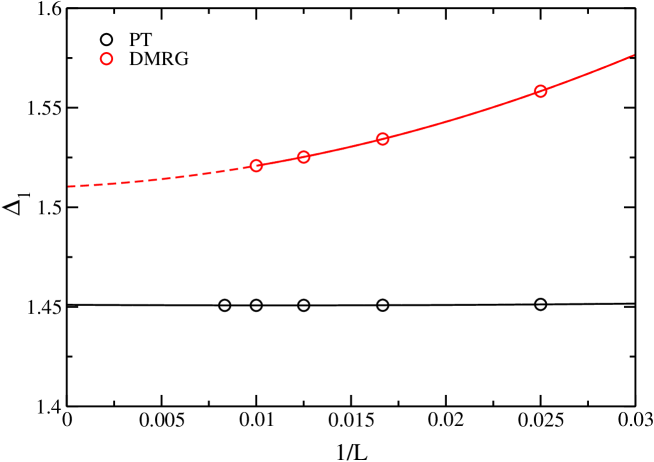
Figure 5: Single-particle gap $\Delta_{1}$ as a function of the inverse system size for fixed $U=2V=2t$ and $\delta=0.2$ in the DMRG and perturbation theory; lines are polynomial fits.

4.2.2 Fixed ratio $U/V$.

Fig. 6 compares the single-particle gap as a function of $V$ for fixed ratio $U/V=2$ in the DMRG and perturbation theory to first and second order. The agreement is worse than for the ground-state energy. Nevertheless, the deviation between the numerically exact DMRG results and perturbation theory at $U=3t$ and $V=1.5t$ is only about ten percent despite the fact that the gap has increased from its noninteracting value $\Delta^{\rm P}=0.8t$ by a factor of 2.5 to $\Delta_{1}^{\rm DMRG}(U=3t,V=1.5t,\delta=0.2)\approx 2.0t$.

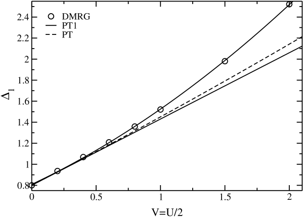
Figure 6: Single-particle gap $\Delta_{1}$ as a function of $V$ for fixed $U/V=2$, $L=100$, and $\delta=0.2$ in the DMRG (circles) and perturbation theory. Lower curve: perturbation theory to first order (PT1), upper curve: perturbation theory to second order (PT). Lines are polynomial fits.

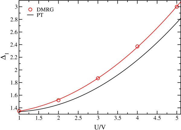
Figure 7: Single-particle gap $\Delta_{1}$ as a function of $U/V$ for $V=t$, $L=100$, and $\delta=0.2$ in the DMRG (circles) and perturbation theory; lines are polynomial fits.

The figure also shows that the second-order contribution only slightly improves the first-order result. The surprisingly good first-order result is partially due to the error compensation in the calculation of the ground-state energies for $N=L$ and $N=L+1$ particles.

4.2.3 Fixed $V$.

As in the case of the ground-state energy, the discrepancies between the DMRG single-particle gap and the result from second-order perturbation theory are mainly caused by the long-range part of the Coulomb interaction. This is shown in Fig. 7. The results from second-order perturbation theory closely follow the DMRG data for all $U/t$ at fixed $V=t$.

At $U=3t$ and $V=t$ the difference between $\Delta_{1}^{\rm DMRG}(U=3t,V=t,\delta=0.2)=1.8680t$ and $\Delta_{1}^{\rm PT}(U=3t,V=t,\delta=0.2)=1.7229t$ is only eight percent. Here, first-order perturbation theory gives $\Delta_{1}^{\rm PT1}(U=3t,V=t,\delta=0.2)=1.430t$ which is off by 23 percent. This shows that the inclusion of the second-order terms improves the agreement considerably for all $U/t$ as long as $V/t$ is not too large.

4.2.4 Conclusion.

Second-order perturbation theory provides a reliable estimate for the single-particle gap in the regime where it has almost tripled from its bare Peierls value, i.e., in the region ($U\leq 4t$, $V\leq 2t$) for $\delta=0.2t$ ($\Delta^{\rm P}=0.8t$). This is rather important because it indicates that only a minor part of the single-particle gap in polymers is caused by the Peierls effect. For poly-acetylene where $t\approx 2\,{\rm eV}$ and $\Delta_{1}\approx 1.6\,{\rm eV}$ one would obtain $\delta=0.2$ in the absence of Coulomb correlations. When we assume a correlation enhancement for the gap by a factor of about three, we would estimate $\delta\approx 0.07$, in agreement with other estimates in the literature.

A reliable estimate for the single-particle gap is important for the calculation of binding energies of bound particle-hole excitations (excitons). They are the subject of the next section.

5 Perturbative approaches to optical excitations

There are various possibilities to set up second-order perturbation theory for optical excitations. In this work we discuss Wannier, two-step, and down-folding perturbation theories separately before we calculate matrix elements. Starting point is the subspace of optical excitations in the Peierls model,

$${\rm singlet}:\quad|s\rangle = \sum_{k}w_{s}(k)|k\rangle_{s}\;,$$

$${\rm triplet}:\quad|t\rangle = \sum_{k}w_{t}(k)|k\rangle_{t}\;,$$ (40)

with the normalization $\sum_{k}[w_{(s,t)}(k)]^{2}=1$ and

$$|k\rangle_{(s,t)}\equiv\sqrt{\frac{1}{2}}\left(\hat{b}_{k,\uparrow}^{+}\hat{a}_{k,\uparrow}\pm\hat{b}_{k,\downarrow}^{+}\hat{a}_{k,\downarrow}\right)|{\rm FS}\rangle\;.$$ (41)

Here, we introduce linear combinations of single particle-hole excitations $|10\rangle$ and $|01\rangle$ from the outset because we are mainly interested in bound states of particle and hole.

5.1 Wannier perturbation theory

Let $\hat{P}$ and $\hat{Q}$ be projectors onto separate subspaces of the Hilbert space, $\hat{P}+\hat{Q}=\hat{1}$. In the case of excitons we let $\hat{P}$ project onto the subspace of a single particle-hole excitation, $\hat{P}\equiv\hat{P}_{1}$. Then, we may write for $\hat{H}=\hat{T}+\hat{W}$

$$\hat{H} = \left[\hat{T}+\hat{P}\hat{W}\hat{P}\right]+\left[\hat{Q}\hat{W}\hat{P}+\hat{P}\hat{W}\hat{Q}+\hat{Q}\hat{W}\hat{Q}\right]$$ (42)

$$\equiv \hat{H}_{0}+\hat{H}_{\perp}\;,$$

where $\hat{H}_{0}$ describes the unperturbed system and $\hat{H}_{\perp}$ represents the perturbation.

5.1.1 Wannier perturbation theory to first order.

In the usual Wannier theory, one diagonalizes $\hat{H}_{0}$ in the subspace of a single particle-hole excitation,

$$\hat{H}_{0}|(s,t)\rangle_{n}=\epsilon_{n}^{(s,t)}|(s,t)\rangle_{n}\;,$$ (43)

where $\epsilon_{n}^{(s,t)}$ is the Wannier spectrum in the spin singlet and triplet sector. Typically, the states with lowest energy correspond to bound states (excitons) [12].

5.1.2 Wannier perturbation theory to second order.

Given the Wannier spectrum and states to first order, we can calculate the Coulomb corrections to the Wannier eigenstates via perturbation theory to second order in $\hat{H}_{\perp}$

$$E_{n}=\epsilon_{n}+\sum_{|m\rangle}\frac{\langle x_{n}|\hat{H}_{\perp}|m\rangle\langle m|\hat{H}_{\perp}|x_{n}\rangle}{\epsilon_{n}-E_{m}^{(0)}}$$ (44)

in the singlet and triplet sector, $x=(s,t)$. Here, $E_{m}^{(0)}=\langle m|\hat{H}_{0}|m\rangle$, and $|m\rangle$ can be chosen as an eigenstate of the Peierls Hamiltonian $\hat{T}$ because corrections are of higher order in the Coulomb interaction. The states $|m\rangle$ contain up to three particle-hole excitations. The corresponding matrix elements in (44) are calculated in the next section.

5.2 Two-step perturbation theory

The Wannier theory for excitons probes how a bound excitation of bare particles and holes is perturbed by the Coulomb interaction. In two-step perturbation theory the two steps are reversed: excitons are formed from dressed particles and holes. This two-step approach is very similar in spirit to the GW-BSE approach where the Bethe–Salpeter Equation is solved for quasi-particles which are calculated in the GW-approximation [9].

To set up the two-step perturbation theory in general, we split the Coulomb interaction into two parts, $\hat{W}=\hat{V}_{A}+\hat{V}_{B}$. Let $\hat{P}_{r}$ be the projection operators onto subspaces with $r$ particle-hole pairs and $\hat{Q}_{r}=\hat{1}-\hat{P}_{r}$ its complement. We identify

$$\hat{V}_{A} = \hat{P}_{r}\hat{W}\hat{Q}_{r}+\hat{Q}_{r}\hat{W}\hat{P}_{r}+\hat{Q}_{r}\hat{W}\hat{Q}_{r}\;,$$ (45)

$$\hat{V}_{B} = \hat{P}_{r}\hat{W}\hat{P}_{r}\;.$$ (46)

In the first step of the perturbation theory we calculate the change of an eigenstate $|n^{0}\rangle$ of $\hat{T}$ due to the influence of the perturbation $\hat{V}_{A}$. In Rayleigh–Schrödinger perturbation theory for $\hat{H}_{A}=\hat{T}+\hat{V}_{A}$ to first order we find

$$|n\rangle=Z_{n}\left\{|n^{0}\rangle+\sum_{|m\rangle}\frac{|m\rangle\langle m|\hat{V}_{A}|n^{0}\rangle}{E_{n^{0}}^{(0)}-E_{m}^{(0)}}\right\}\;.$$ (47)

To second order the normalization factor $Z_{n}$ reads

$$|Z_{n}|^{2}=1-\sum_{|m\rangle}\frac{\left|\langle n^{0}|\hat{V}_{A}|m\rangle\right|^{2}}{\left(E_{n^{0}}^{(0)}-E_{m}^{(0)}\right)^{2}}\;.$$ (48)

The states $|n\rangle$ are so-called ‘dressed states’ because they contain particle-hole excitations which are renormalized by the interaction $\hat{V}_{A}$.

In the second step we apply (almost degenerate) perturbation theory for the perturbation $\hat{V}_{B}$. Therefore, we diagonalize $\hat{H}=\hat{H}_{A}+\hat{V}_{B}$ in the basis of the states $|n\rangle$, i.e., we calculate the eigenvalues of the Hamilton matrix

$$H(n_{1},n_{2})=\langle n_{1}|\hat{H}|n_{2}\rangle$$ (49)

in the respective subspaces with $r$ particle-hole excitations.

As an example we consider the case $r=0$, i.e., we calculate the second-order ground-state energy in two-step perturbation theory. Since $|0\rangle$ is not degenerate, we have

$$|0^{0}\rangle = |{\rm FS}\rangle\;,$$ (50)

$$|0\rangle = Z_{0}(|{\rm FS}\rangle+|X\rangle)\;.$$ (51)

The Hamilton matrix is a scalar,

$$E_{0} = \langle 0|\hat{H}|0\rangle$$ (52)

$$= \left(|Z_{0}|^{2}-1\right)\langle{\rm FS}|\hat{T}|{\rm FS}\rangle+\langle{\rm FS}|\hat{T}+\hat{W}|{\rm FS}\rangle$$

$$+\langle X|\hat{W}|{\rm FS}\rangle+\langle{\rm FS}|\hat{W}|X\rangle+\langle X|\hat{T}|X\rangle$$

$$= \langle{\rm FS}|\hat{T}+\hat{W}|{\rm FS}\rangle+\sum_{|m\rangle\neq|{\rm FS}\rangle}\frac{\left|\langle{\rm FS}|\hat{W}|m\rangle\right|^{2}}{E_{0}^{(0)}-E_{m}^{(0)}}\;.$$

This expression is identical to Rayleigh–Schrödinger perturbation theory to second order.

5.3 Down-folding perturbation theory

5.3.1 Equivalence to Brillouin–Wigner perturbation theory.

The so-called ‘down-folding’ approach is also based on a projection to relevant degrees of freedom. Consider the stationary Schrödinger equation at energy $E$

$$\hat{H}|\Psi\rangle=\left(\hat{T}+\hat{W}\right)|\Psi\rangle=E|\Psi\rangle\;.$$ (53)

For any two projectors $\hat{P}$ and $\hat{Q}$ with $\hat{P}+\hat{Q}=\hat{1}$ we define the orthogonal states

$$|\varphi\rangle=\hat{P}|\Psi\rangle\quad,\quad|\chi\rangle=\hat{Q}|\Psi\rangle$$ (54)

which obey the coupled Schrödinger equations

$$E|\varphi\rangle = \hat{P}\hat{H}|\varphi\rangle+\hat{P}\hat{H}|\chi\rangle\;,$$

$$E|\chi\rangle = \hat{Q}\hat{H}|\varphi\rangle+\hat{Q}\hat{H}|\chi\rangle\;.$$ (55)

The second equation is formally inverted with the help of the resolvent operator $(z-\hat{H})^{-1}$ to give a single equation

$$\hat{P}\hat{H}\hat{P}|\varphi\rangle+\hat{P}\hat{H}\hat{Q}\left(E-\hat{H}\right)^{-1}\hat{Q}\hat{H}\hat{P}|\varphi\rangle=E|\varphi\rangle\;.$$ (56)

We now set $\hat{P}\equiv\hat{P}_{r}$ so that

$$\hat{P}_{r}\hat{H}\hat{P}_{r}=\hat{T}+\hat{P}_{r}\hat{W}\hat{P}_{r}\;,\;\hat{P}_{r}\hat{H}\hat{Q}_{r}=\hat{P}_{r}\hat{W}\hat{Q}_{r}\;,\;\hat{Q}_{r}\hat{H}\hat{P}_{r}=\hat{Q}_{r}\hat{W}\hat{P}_{r}\,,$$ (57)

and insert the unit operator in (56) to obtain

$$\hat{P}_{r}\hat{H}\hat{P}_{r}|\varphi\rangle+\sum_{|m\rangle}\frac{\hat{P}_{r}\hat{W}\hat{Q}_{r}|m\rangle\langle m|\hat{Q}_{r}\hat{W}_{r}\hat{P}_{r}|\varphi\rangle}{E_{\varphi}-E_{m}}=E_{\varphi}|\varphi\rangle\;.$$ (58)

The same expression is obtained in Brillouin–Wigner perturbation theory in which the energy $E\equiv E_{\varphi}$ must be determined self-consistently.

5.3.2 Size-consistent reformulation.

The down-folding or Brillouin–Wigner perturbation expansion is hampered by the fact that it is not size-consistent. Therefore, the form (58) cannot be used for our calculations.

In order to make progress, we first subtract the ground-state energy from all energies in (58),

$$(E_{\varphi}-E_{0})|\varphi\rangle=\hat{P}_{r}(\hat{H}-E_{0})|\varphi\rangle+\sum_{|m\rangle}\frac{\hat{P}_{r}\hat{W}\hat{Q}_{r}|m\rangle\langle m|\hat{Q}_{r}\hat{W}|\varphi\rangle}{(E_{\varphi}-E_{0})-(E_{m}-E_{0})}\;,$$ (59)

so that all energy differences correspond to excitation energies of order unity. To second order in the interaction we may write

$$E_{\varphi}-E_{0}\equiv e_{\varphi}\quad,\quad E_{m}-E_{0}=E_{m}^{(0)}-E_{0}^{(0)}+{\cal O}(U,V)\;.$$ (60)

Therefore, to second order we find

$$e_{\varphi}|\varphi\rangle=\hat{P}_{r}(\hat{H}-E_{0})|\varphi\rangle+\sum_{|m\rangle}\frac{\hat{P}_{r}\hat{W}\hat{Q}_{r}|m\rangle\langle m|\hat{Q}_{r}\hat{W}|\varphi\rangle}{e_{\varphi}-(E_{m}^{(0)}-E_{0}^{(0)})}\;.$$ (61)

As an example, we apply this equation for the ground state, i.e., $r=0$, $|\varphi\rangle=|{\rm FS}\rangle$, and $e_{\varphi}=0$. When we multiply (61) from the left with $\langle{\rm FS}|$ we immediately recover the result from Rayleigh–Schrödinger perturbation theory.

For the exciton states $|x\rangle$ and energies $e_{x}$ we find the Schrödinger equation

$$e_{x}|x\rangle=\hat{P}_{1}(\hat{H}-E_{0})|x\rangle+\sum_{|m\rangle}\frac{\hat{P}_{1}\hat{W}\hat{Q}_{1}|m\rangle\langle m|\hat{Q}_{1}\hat{W}|x\rangle}{e_{x}-(E_{m}^{(0)}-E_{0}^{(0)})}\;.$$ (62)

This translates into a matrix-diagonalization problem with the diagonal entries

$$H_{\rm BW}(e_{(s,t)};k_{1},k_{1}) = {}_{(s,t)}\langle k_{1}|\hat{T}|k_{1}\rangle_{(s,t)}-\langle{\rm FS}|\hat{T}|{\rm FS}\rangle-E_{0}^{(2)}$$ (63)

$$+{}_{(s,t)}\langle k_{1}|\hat{W}|k_{1}\rangle_{(s,t)}-\langle{\rm FS}|\hat{W}|{\rm FS}\rangle$$

$$+\sum_{|m\rangle}\frac{{}_{(s,t)}\langle k_{1}|\hat{W}|m\rangle_{(s,t)}{}_{(s,t)}\langle m|\hat{W}|k_{1}\rangle_{(s,t)}}{e_{(s,t)}-(E_{m}^{(0)}-E_{0}^{(0)})}\;,$$

and the non-diagonal entries ($k_{1}\neq k_{2}$)

$$H_{\rm BW}(e_{(s,t)};k_{1},k_{2}) = {}_{(s,t)}\langle k_{1}|\hat{W}|k_{2}\rangle_{(s,t)}$$

$$+\sum_{|m\rangle}\frac{{}_{(s,t)}\langle k_{1}|\hat{W}|m\rangle_{(s,t)}{}_{(s,t)}\langle m|\hat{W}|k_{2}\rangle_{(s,t)}}{e_{(s,t)}-(E_{m}^{(0)}-E_{0}^{(0)})}\;,$$

where the excited states $|m\rangle$ contain none, two, or three particle-hole excitations of the Peierls ground state. Note that the eigenvalue $e_{(s,t)}$ of the matrix $H_{\rm BW}(e_{(s,t)})$ in (LABEL:heff_mat) must be determined self-consistently. In our calculations we target the lowest eigenvalue as the bound exciton in the triplet and singlet sectors.

6 Excitons to second order

6.1 Analytical results

The calculation of optical excitation energies requires the matrix elements

$$M_{0,(s,t)}(p_{1},p_{2})={}_{(s,t)}\langle p_{1}|\hat{T}|p_{2}\rangle_{(s,t)}-\delta_{p_{1},p_{2}}E_{0}^{(0)}=\delta_{p_{1},p_{2}}2E(p_{1})\;,$$ (65)

and

$$M_{1,(s,t)}(p_{1},p_{2}) = {}_{(s,t)}\langle p_{1}|\hat{W}|p_{2}\rangle_{(s,t)}-\delta_{p_{1},p_{2}}E_{0}^{(1)}\;,$$ (66)

$$M_{2,(s,t)}(e;p_{1},p_{2}) = \sum_{|m\rangle}\frac{{}_{(s,t)}\langle p_{1}|\hat{W}|m\rangle_{(s,t)}{}_{(s,t)}\langle m|\hat{W}|p_{2}\rangle_{(s,t)}}{e-(E_{m}^{(0)}-E_{0}^{(0)})}\;,$$ (67)

where $|m\rangle$ contains up to three particle-hole excitations.

6.1.1 Matrix elements to first order.

The matrix elements $M_{1}$ are readily calculated. We find

$$M_{1,(s,t)}(p_{1},p_{2})=M_{1,(s,t)}^{U}(p_{1},p_{2})+M_{1,(s,t)}^{V}(p_{1},p_{2})$$ (68)

with

$$M_{1,(s,t)}^{U}(p_{1},p_{2})=\pm\frac{U}{L}\;,$$ (69)

and

$$M_{1,(s,t)}^{V}(p_{1},p_{2}) = \delta_{p_{1},p_{2}}\sum_{-L/2<r<L/2\atop{r|2=1}}V(r)\Bigl{[}\frac{8\cos(p_{1})\cos(p_{1}r)}{E(p_{1})}A_{\delta}(r)$$ (70)

$$\hphantom{\frac{1}{2}\sum_{-L/2<r<L/2\atop{r|2=1}}V(r)\delta_{p_{1},p_{2}}}+\frac{8\delta\sin(p_{1})\sin(p_{1}r)}{E(p_{1})}B_{\delta}(r)\Bigr{]}$$

$$-\frac{2}{L}\sum_{r\neq 0}V(r)\cos((p_{1}-p_{2})r)$$

$$\hphantom{-\frac{2}{L}\sum_{r\neq 0}}\left[f_{2}^{2}(p_{1},p_{2})+(-1)^{r}f_{1}^{2}(p_{1},p_{2})\right]$$

$$+\frac{2}{L}\sum_{r\neq 0}V(r)\left[1+(1\pm 1)(-1)^{r}\right]\;.$$

6.1.2 Matrix elements to second order.

The intermediate states $|00\rangle=|{\rm FS}\rangle$, $|11\rangle$, $|20\rangle$, $|02\rangle$, $|30\rangle$, $|03\rangle$, $|21\rangle$, and $|12\rangle$ contribute to (67). The respective terms are lengthy, see B. As in sections 3 and 4 we write

$$M_{2,(s,t)}(e;p_{1},p_{2}) = M_{2,(s,t)}^{U^{2}}(e;p_{1},p_{2})+M_{2,(s,t)}^{V^{2}}(e;p_{1},p_{2})$$ (71)

$$+M_{2,(s,t)}^{UV}(e;p_{1},p_{2})\;.$$

The contributions to $M_{2,(s,t)}^{U^{2}}(e;p_{1},p_{2})$ can be found in (92) and (B.1). The terms for $M_{2,(s,t)}^{V^{2}}(e;p_{1},p_{2})$ result from (94), (95), (96), (98), and (97). Lastly, the terms for $M_{2,(s,t)}^{UV}(e;p_{1},p_{2})$ are collected in (99) and (100).

6.1.3 Wannier perturbation theory.

The first-order result from Wannier perturbation theory for the singlet/triplet excitons follows from the lowest eigenvalue $e_{(s,t)}^{(1)}$ of the Wannier matrix with entries

$$M^{\rm W}(p_{1},p_{2})=M_{0,(s,t)}(p_{1},p_{2})+M_{1,(s,t)}(p_{1},p_{2})\;.$$ (72)

Moreover, this calculation gives the first-order Wannier wave functions with (real) amplitudes $w_{(s,t)}(p)$, cf. (40).

To second order, we evaluate (44),

$$e_{(s,t)}^{(2)}=\sum_{|m\rangle}\frac{\langle(s,t)|\hat{H}_{\perp}|m\rangle\langle m|\hat{H}_{\perp}|(s,t)\rangle}{e_{(s,t)}^{(0)}-(E_{m}^{(0)}-E_{0}^{(0)})}\;.$$ (73)

On the right-hand-side of this equation we keep only the kinetic energy of the Wannier exciton,

$$e_{(s,t)}^{(0)}=\sum_{k}2E(k)[w_{(s,t)}(k)]^{2}$$ (74)

in order to be consistent to second order in the Coulomb interaction. The second-order correction of the Wannier excitons’ excitation energy is then given by

$$e_{(s,t)}^{(2)}=\sum_{p_{1},p_{2}}w_{(s,t)}(p_{1})w_{(s,t)}(p_{2})M_{2,(s,t)}(e_{(s,t)}^{(0)};p_{1},p_{2})-E_{0}^{(2)}\;,$$ (75)

and the excitons’ excitation energy is $e_{(s,t)}=e_{(s,t)}^{(1)}+e_{(s,t)}^{(2)}$.

6.1.4 Two-step perturbation theory.

To first order, the results from the Wannier and two-step perturbation theories are identical. For the calculation of the corrections we define the matrix

$$B_{(s,t)}(p_{1},p_{2}) = \sum_{|m\rangle}{}_{(s,t)}\langle p_{1}|\hat{W}|m\rangle\langle m|\hat{W}|p_{2}\rangle_{(s,t)}$$

$$\frac{E_{m}^{(0)}-E_{0}^{(0)}}{(2E(p_{1})-(E_{m}^{(0)}-E_{0}^{(0)}))(2E(p_{2})-(E_{m}^{(0)}-E_{0}^{(0)}))}\;.$$

In order to calculate the entries of this matrix the energy denominators which appear in B must be modified appropriately.

As shown in (49), the excitation energy of the excitons in two-step perturbation theory is then obtained from the lowest eigenvalues of the matrix with the entries

$$A_{(s,t)}(p_{1},p_{2}) = M_{0,(s,t)}(p_{1},p_{2})+M_{1,(s,t)}(p_{1},p_{2})$$ (77)

$$+\delta_{p_{1},p_{2}}\left(M_{2,(s,t)}(2E(p_{1});p_{1},p_{1})-E_{0}^{(2)}\right)$$

$$+(1-\delta_{p_{1},p_{2}})\Bigl{(}M_{2,(s,t)}(2E(p_{1});p_{1},p_{2})$$

$$\hphantom{+(1-\delta_{p_{1},p_{2}})\Bigl{(}}+M_{2,(s,t)}(2E(p_{2});p_{1},p_{2})$$

$$\hphantom{+(1-\delta_{p_{1},p_{2}})\Bigl{(}}+B_{(s,t)}(p_{1},p_{2})\Bigr{)}\;.$$

6.1.5 Down-folding perturbation theory.

According to (63) and (LABEL:heff_mat) the down-folding method requires the diagonalization of the matrix with the entries

$$F_{(s,t)}(e_{(s,t)};p_{1},p_{2}) = M_{0,(s,t)}(p_{1},p_{2})+M_{1,(s,t)}(p_{1},p_{2})$$ (78)

$$+M_{2,(s,t)}(e_{(s,t)};p_{1},p_{2})-\delta_{p_{1},p_{2}}E_{0}^{(2)}\;.$$

The lowest eigenvalue must be determined self-consistently.

6.1.6 Comparison of numerical effort.

The numerically cheapest method is the two-step perturbation theory. For given Peierls dimerization $\delta$ and functional form of $V(r)$ one can calculate and store the matrix elements which define $A_{(s,t)}(p_{1},p_{2})$. The parameters $U$, $V$ only enter as multiplicative factors.

This does not hold for the Wannier approach anymore because the kinetic energy depends on the wave function of the Wannier exciton in first order of the interaction. For a first guess we could replace $e_{(s,t)}^{(0)}$ in (74) by $2E(-\pi/2)$ because $p=-\pi/2$ is the dominant contribution in the excitonic wave functions. This speeds up the analysis as a function of the Coulomb parameters but it also reduces the quality of the results.

The down-folding approach is the most costly of the three approaches in terms of computer-time. For given interaction parameters, the effort of the second-order Wannier theory has to be repeated some six to eight times until convergence is reached.

6.2 Comparison with numerical results for the singlet exciton

We start with a comparison of our analytical results for the singlet exciton with those of the DMRG. For the latter we assume that the singlet exciton is identical to the lowest-lying charge excitation at fixed particle number $N=L$. This assumption is justified in the presence of a singlet exciton.

We do not present results from the down-folding approach. The self-consistency algorithm is stable but the results from the down-folding approach underestimate the excitonic excitation energies drastically. We do not consider the down-folding perturbation theory any further because it is numerically the most expensive and quantitatively the least successful of our perturbative approaches.

6.2.1 Finite-size effects.

As in previous sections we first investigate the size-dependence of the excitation energy. In Fig. 8 we compare the results from the DMRG with those from the various perturbative approaches which we discussed in section 5. The DMRG data show a very weak size dependence which is a clear signal for a bound state. The data PT and PT1 do not reproduce this $1/L$ dependence. In fact, they describe an unbound particle-hole excitation. The starting point for PT and PT1 is a single particle-hole excitation at momentum $p=-\pi/2$, and corrections are calculated in first and second-order Rayleigh–Schrödinger perturbation theory, respectively. The results show that this approach is not applicable for the description of excitonic optical excitations, and we shall not pursue this approach any further.

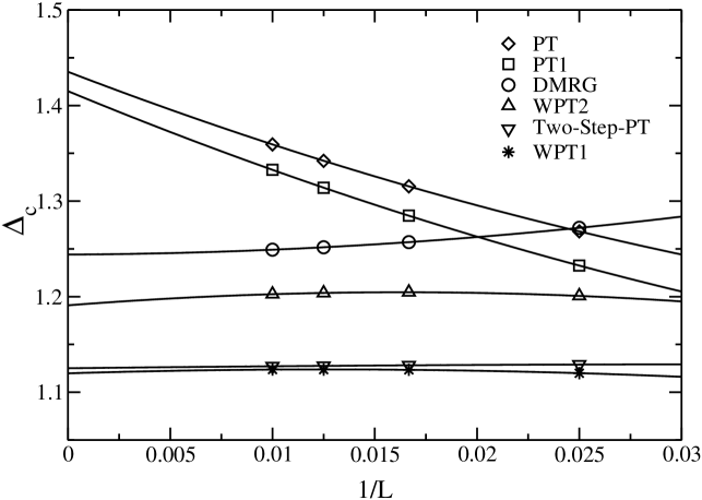
Figure 8: Singlet exciton energy (charge gap) $\Delta_{c}$ as a function of inverse system size for fixed $U=2V=2t$ and $\delta=0.2$ in the DMRG and perturbation theory; see text for further details.

Wannier theory to first order (WPT1), to second order (WPT2), and the two-step perturbation theory show a very weak size dependence, characteristic for a bound state. As seen from the figure, the two-step perturbation theory does not improve the result from first-order Wannier perturbation theory, and the second-order Wannier theory is the best approximation to the DMRG data.

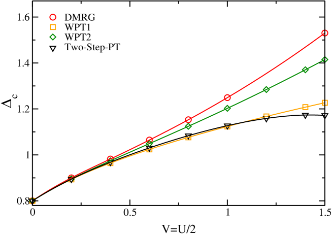
Figure 9: Singlet exciton energy (charge gap) $\Delta_{c}$ as a function of $V$ for fixed ratio $U/V=2$, $L=100$, and $\delta=0.2$ in the DMRG and in various perturbative approaches.

In all cases, the results for $L=100$ are a very good estimate for the results in the thermodynamic limit. The differences between the various perturbative approaches and the numerically exact DMRG are significant.

6.2.2 Fixed ratio $U/V$.

In Fig. 9 we show the results for the singlet excitation energy as a function of $V$ for $L=100$, $\delta=0.2$, and fixed ratio $U/V=2$. It is seen that second-order Wannier theory is naturally superior to the first order approximation and provides a rather good description. At ($V=1.5t$, $U=3t$), when the charge gap has almost doubled from its non-interacting value $\Delta^{\rm P}$, the difference between the DMRG and second-order Wannier theory is less than ten percent. In contrast, the first-order Wannier theory is already off by 30 percent, and two-step perturbation theory becomes even worse than that.

6.2.3 Fixed $V$.

As for the ground-state energy and the single-particle gap, the discrepancies between the DMRG and second-order perturbation theory increase as a function of $V$ but not so much as a function of $U$. In Fig. 10 we show the singlet excitation energy as a function of $U$ for fixed $V=t$, $L=100$, and $\delta=0.2$. The two-step perturbation theory and second-order Wannier theory closely follow the almost quadratical increase of the charge gap as a function of $U$. The singlet excitation energy can triple from its bare value $\Delta^{\rm P}=0.8t$ at ($U=5t$, $V=t$), and still the deviations are only about ten percent. In contrast, first-order Wannier theory begins to deviate noticeably already at ($U=3t,V=t$).

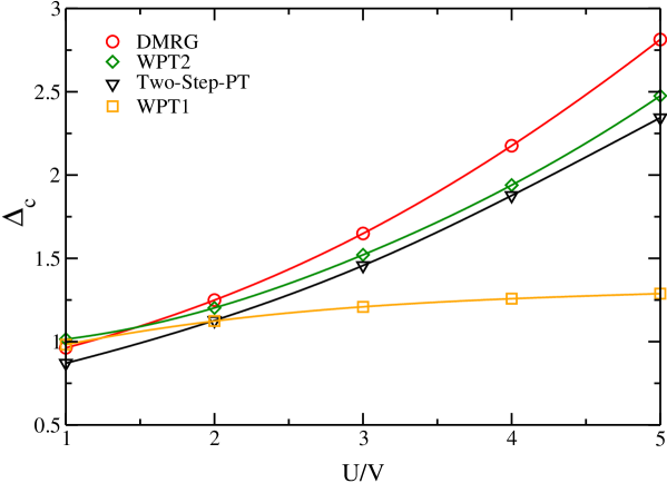
Figure 10: Singlet exciton energy (charge gap) $\Delta_{c}$ as a function of $U/V$ for fixed $V=t$, $L=100$, and $\delta=0.2$ in the DMRG and in various perturbative approaches.

6.2.4 Conclusion.

Wannier theory to second order consistently improves the results from first-order Wannier theory. It provides a quantitative description even for large Coulomb parameters when the charge gap has more than doubled from its bare Peierls value.

The two-step perturbation theory can handle the influence of large Hubbard interactions but it fails quickly when the long-range parts of the Coulomb interactions become relevant. This is somewhat unfortunate because the two-step perturbation theory is numerically the cheapest of all second-order methods.

The good performance of the second-order Wannier theory indicates that this approach describes the relevant objects appropriately. To first order in the Coulomb interaction Wannier theory forms the charge neutral exciton from a negative (electron) and a positive charge excitation (hole). This object has the appropriate quantum numbers also for strong Coulomb interactions. Therefore, the residual Coulomb interactions, i.e, the coupling to the ground state and other particle-hole excitations, apparently perturb the exciton properly. In contrast, two-step perturbation theory builds excitons from dressed electrons and holes and thereby overestimates the repulsion against other states with electron-hole pairs which results in a too small energetic splitting between the exciton in two-step perturbation theory and the ground state.

6.3 Comparison with numerical results for the triplet exciton

We continue with a comparison of our analytical results for the triplet exciton with those of the DMRG. For the latter we assume that the triplet exciton is identical to the lowest-lying spin excitation at fixed particle number $N=L$. This assumption is justified in the presence of a triplet exciton. Again, we do not present results from the down-folding approach because it fails quantitatively already for fairly small interaction strengths.

6.3.1 Fixed ratio $U/V$.

For the triplet exciton, the results from perturbation theory are much less reliable than for the singlet exciton. As can be seen from Fig. 11, a quantitatively correct answer is provided by second-order Wannier theory only up to $U=2V=2t$, whereas first-order Wannier theory and two-step perturbation theory fail for even smaller Coulomb parameters.

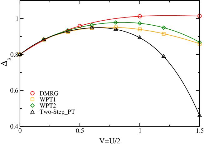
Figure 11: Triplet exciton energy (spin gap) $\Delta_{s}$ as a function of $V$ for fixed ratio $U/V=2$, $L=100$, and $\delta=0.2$ in the DMRG and in various perturbative approaches.

6.3.2 Fixed $V$.

Perturbation theory fails even qualitatively for moderate to large values of the Hubbard interaction. The DMRG exciton energy increases, flattens out, and finally turns into a $1/U$ behavior, as seen in Figs. 11 and 12. This shows that the nature of the excitonic excitation changes drastically as a function of $U/t$: for large Coulomb interactions the triplet exciton is a bound state of a pair of two spins on singly occupied sites, i.e., it looses its character of bound charge excitations which is assumed in perturbation theory.

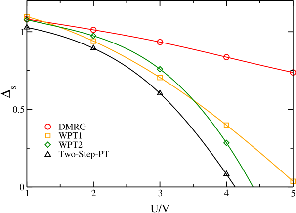
Figure 12: Triplet exciton energy (spin gap) $\Delta_{s}$ as a function of $U/V$ for fixed $V=t$, $L=100$, and $\delta=0.2$ in the DMRG and in various perturbative approaches.

6.3.3 Conclusion.

Triplet excitons cannot be described reliably within low-order perturbation theory because the nature of the lowest triplet excitation quickly changes as a function of the interaction strength. For not too large Hubbard interactions, the triplet exciton looses its charge contents and is better viewed as a bound state of two spin-1/2 excitations (spinons). The description of such a state lies beyond the possibilities of finite-order perturbation theory.

7 Concluding remarks

7.1 Summary

In this work we performed second-order perturbation theory for the extended Peierls–Hubbard model for the ground-state energy and the single-particle gap. The agreement with the numerically exact DMRG data was very good up to Coulomb parameters where the bare Peierls gap has almost tripled.

For bound optical excitations, the situation is less favorable. The singlet exciton energy is reasonably well described by second-order Wannier perturbation theory for Coulomb parameters which lead to a doubling of the single-particle gap. The triplet exciton can be described perturbatively for weak coupling only.

The second-order Wannier theory proves to be superior to other second-order approaches. Its success may be related to the fact that after its formation the exciton is a charge neutral object to which other parts of the Hilbert space are coupled less intensely by the Coulomb interaction. The computationally most costly down-folding method performs worst and can be safely discarded. The two-step perturbation theory where excitons are formed from dressed particles is computationally the cheapest method. Unfortunately, it does not improve the first-order Wannier theory for the singlet exciton systematically. This indicates that the exciton should not be seen as a bound state of dressed quasi-particles. In order to investigate this question further, the GW-BSE approach [9] ought to be applied directly to the extended Peierls–Hubbard model so that its predictions can be tested against the numerically exact DMRG results.

7.2 Discussion

In order to compare our results with those of previous work on poly-(di)acetylene, we note that we may write $V=e^{2}/(\varepsilon a_{0})$ where $a_{0}\approx 1.4$Å is the average distance between the carbon atoms, $e$ is the electric charge and $\varepsilon$ is the dielectric constant of the surrounding medium. In [8] its value is given by $\varepsilon_{\rm Abe}\approx 5$ which is much larger than the typical values for plastic, $\varepsilon\approx 2.3$. For the Abe value one finds $V\approx 2\,{\rm eV}=t$, and the application of first-order (Wannier) perturbation theory at $\delta=0.2$ gives a reasonable agreement with the measured binding energies of the first singlet and triplet exciton in poly-diacetylene which are $\Delta_{\rm c}=0.5\,{\rm eV}$ and $\Delta_{\rm s}=0.9\,{\rm eV}$, respectively. However, the measured single-particle gap is $\Delta_{1}=2.3\,{\rm eV}$ which is seriously overestimated by $0.7\,{\rm eV}$ for the given choice of parameters, $\Delta_{1}^{\rm DMRG}(U=2t,V=t,\delta=0.2)=3.0\,{\rm eV}$.

The reason for this discrepancy is readily identified. The assumption $\delta=0.2$ leads to a bare gap of $\Delta_{\rm P}=0.8t\approx 1.6\,{\rm eV}$. As has been seen in Fig. 6, the single-particle gap increases linearly with the Coulomb interaction. Therefore, a good agreement with the experimental gap value is achieved at $V=0.6t$ which would correspond to $\varepsilon\approx 8$ which is unrealistic. Apparently, the assumption of a large Peierls gap is not correct.

A more realistic approach starts from a much smaller Peierls contribution to the gap. We should rather work with $\delta=0.1$ or smaller [13], which is in accordance with an estimate of the electron-lattice interaction in benzene [7]. The Peierls gap then is $\Delta_{\rm P}=0.4t\approx 0.8\,{\rm eV}$ which is about one third of the full gap. We then find for the single-particle gap $\Delta_{1}^{\rm PT}(U=2t,V=t,\delta=0.1)=1.75\,{\rm eV}$ from second-order perturbation theory which is 12 percent below the exact value of $\Delta_{1}^{\rm DMRG}(U=2t,V=t,\delta=0.1)=1.98\,{\rm eV}$ from the DMRG. For the singlet exciton, we find $\Delta_{\rm c}^{\rm PT}(U=2t,V=t,\delta=0.1)=1.44\,{\rm eV}$ which is 22 percent above the DMRG value $\Delta_{\rm c}^{\rm DMRG}(U=2t,V=t,\delta=0.1)=1.18\,{\rm eV}$. The agreement is quite acceptable in both cases. However, the comparison of the binding energies for the singlet exciton, $\Delta_{\rm bind,s}^{\rm PT}(U=2t,V=t,\delta=0.1)=0.31\,{\rm eV}$ versus $\Delta_{\rm bind,s}^{\rm DMRG}(U=2t,V=t,\delta=0.1)=0.80\,{\rm eV}$ reveals that we are stretching second-order perturbation theory beyond its limits because the error in the binding energy increases to more than 60 percent.

A realistic description of the experimental data for poly-diacetylene requires the inclusion of the full band-structure and of the lattice relaxation for excited states, mostly for the triplet exciton [14]. In particular, a better understanding of the screening in these materials [15] and a refinement of the Ohno potential are necessary.

Appendix A Useful relations

A.1 Peierls transformation

The Peierls Hamiltonian is diagonalized via the transformation

$$\hat{a}_{k,\sigma}=\alpha_{k}\hat{c}_{k,\sigma}+{\rm i}\beta_{k}\hat{c}_{k+\pi,\sigma}\;,\quad\hat{b}_{k,\sigma}=\beta_{k}\hat{c}_{k,\sigma}-{\rm i}\alpha_{k}\hat{c}_{k+\pi,\sigma}\;.$$ (79)

Its inverse reads

$$\hat{c}_{k,\sigma}=\alpha_{k}\hat{a}_{k,\sigma}+\beta_{k}\hat{b}_{k,\sigma}\;,quad\hat{c}_{k+\pi,\sigma}=-{\rm i}\beta_{k}\hat{a}_{k,\sigma}+{\rm i}\alpha_{k}\hat{a}_{k,\sigma}\;.$$ (80)

Moreover, we have

$$2\alpha_{k}\beta_{k}=-\frac{2t\delta\sin(k)}{E(k)}\;,\quad\alpha_{k}^{2}-\beta_{k}^{2}=\frac{2t\cos(k)}{E(k)}\;.$$ (81)

A.2 Help functions

In order to express matrix second-order elements for the Hubbard interaction we introduce the abbreviations

$$f_{1}(k_{1},k_{2}) \equiv \alpha_{k_{1}}\beta_{k_{2}}-\alpha_{k_{2}}\beta_{k_{1}}=-f_{1}(k_{2},k_{1})\;,$$

$$f_{2}(k_{1},k_{2}) \equiv \alpha_{k_{1}}\alpha_{k_{2}}+\beta_{k_{1}}\beta_{k_{2}}=f_{2}(k_{2},k_{1})\;,$$

$$u_{1}(k_{1},k_{2},k_{3},k_{4}) \equiv f_{1}(k_{2},k_{1})f_{1}(k_{4},k_{3})-f_{2}(k_{2},k_{1})f_{2}(k_{4},k_{3})\;,$$

$$u_{2}(k_{1},k_{2},k_{3},k_{4}) \equiv f_{1}(k_{2},k_{1})f_{2}(k_{4},k_{3})+f_{1}(k_{4},k_{3})f_{2}(k_{2},k_{1})\;.$$ (82)

The second-order matrix elements for the long-range Coulomb require the functions

$$A_{\delta}(r) \equiv \frac{1}{L}\sum_{k}\frac{\cos(k)\cos(kr)}{\sqrt{\cos(k)^{2}+\delta^{2}\sin(k)^{2}}}=A_{\delta}(-r)\;,$$

$$B_{\delta}(r) \equiv \frac{1}{L}\sum_{k}\frac{\delta\sin(k)\sin(kr)}{\sqrt{\cos(k)^{2}+\delta^{2}\sin(k)^{2}}}=-B_{\delta}(-r)\;,$$ (83)

$$v_{0}(k) \equiv \sum_{-L/2<r<L/2,r|2=1}\frac{1}{2|r|}\frac{4t}{E(k)}\Bigl{(}\delta\sin(k)\cos(kr)A_{\delta}(r)$$ (84)

$$\hphantom{\sum_{-L/2<r<L/2,r|2=1}\frac{1}{2|r|}\frac{4t}{E(k)}\Bigl{(}}-\cos(k)\sin(kr)B_{\delta}(r)\Bigr{)}\;,$$

where ($r|2=1$) denotes all odd $r$. With the help functions

$$C_{+}(k_{1},k_{2}) \equiv \sum_{r\neq 0}\frac{1}{2|r|}2\cos(r(k_{1}-k_{2}))\;,$$

$$C_{-}(k_{1},k_{2}) \equiv \sum_{r\neq 0}\frac{(-1)^{r}}{2|r|}2\cos(r(k_{1}-k_{2}))$$ (85)

we then introduce

$$v_{1}(k_{1},k_{2},k_{3},k_{4}) \equiv C_{+}(k_{3},k_{4})f_{1}(k_{2},k_{1})f_{1}(k_{4},k_{3})$$ (86)

$$-C_{-}(k_{3},k_{4})f_{2}(k_{2},k_{1})f_{2}(k_{4},k_{3})\,;$$

$$v_{2}(k_{1},k_{2},k_{3},k_{4}) \equiv C_{+}(k_{3},k_{4})f_{1}(k_{4},k_{3})f_{2}(k_{2},k_{1})$$ (87)

$$+C_{-}(k_{3},k_{4})f_{1}(k_{2},k_{1})f_{2}(k_{4},k_{3})\;.$$

A.3 Useful contractions

We collect some contractions which frequently appear in the calculation of matrix elements to first and second order in the Coulomb interaction. The expression $\langle\hat{O}\rangle_{0}$ denotes the expectation value of the operator $\hat{O}$ in the ground state $|{\rm FS}\rangle$ (12) of the Peierls insulator. The pair contractions are

$$\langle\hat{n}_{l,\sigma}\rangle_{0} = \frac{1}{2}\;,$$ (88)

$$\langle\hat{c}^{+}_{l,\sigma}\hat{c}_{l+r,\sigma}\rangle_{0} = \frac{1}{2}\delta_{r,0}+\frac{1-(-1)^{r}}{2}(A_{\delta}(r)+(-1)^{l}B_{\delta}(r))\;,$$

$$\langle\hat{c}^{+}_{l,\sigma}\hat{a}_{k,\sigma}\rangle_{0} = \frac{1}{\sqrt{L}}e^{-{\rm i}kl}(\alpha_{k}+{\rm i}(-1)^{l}\beta_{k})\;,$$

$$\langle\hat{c}_{l,\sigma}\hat{b}^{+}_{k,\sigma}\rangle_{0} = \frac{1}{\sqrt{L}}e^{{\rm i}kl}(\beta_{k}+{\rm i}(-1)^{l}\alpha_{k})\;.$$ (89)

Important contractions with four Fermi operators are

$$\langle\hat{n}_{l,\sigma}\hat{b}^{+}_{k_{1},\sigma}\hat{a}_{k_{2},\sigma}\rangle_{0} = \frac{1}{L}e^{{\rm i}(k_{1}-k_{2})l}(f_{1}(k_{2},k_{1})+{\rm i}(-1)^{l}f_{2}(k_{2},k_{1}))\;,$$

$$\langle\hat{b}_{k,\sigma}\hat{c}^{+}_{l+r,\sigma}\rangle_{0}\langle\hat{c}_{l,\sigma}\hat{b}^{+}_{k,\sigma}\rangle_{0} = \frac{1}{L}e^{-{\rm i}kr}(\beta_{k}^{2}+(-1)^{r}\alpha_{k}^{2})$$

$$+{\rm i}\frac{1}{L}e^{-{\rm i}kr}(-1)^{l}(1-(-1)^{r})\alpha_{k}\beta_{k}\;,$$

$$\langle\hat{a}^{+}_{k,\sigma}\hat{c}_{l+r,\sigma}\rangle_{0}\langle\hat{c}^{+}_{l,\sigma}\hat{a}_{k,\sigma}\rangle_{0} = -\frac{1}{L}e^{{\rm i}kr}(\alpha_{k}^{2}+(-1)^{r}\beta_{k}^{2})$$

$$-{\rm i}\frac{1}{L}e^{{\rm i}kr}(-1)^{l}(1-(-1)^{r})\alpha_{k}\beta_{k}\;.$$

and

$$\left\langle\hat{b}_{k_{1},\sigma}\left(\hat{n}_{l,\sigma}-\frac{1}{2}\right)\hat{b}^{+}_{k_{2},\sigma}\right\rangle_{0} = \frac{1}{L}e^{-{\rm i}(k_{1}-k_{2})l}f_{2}(k_{2},k_{1})$$ (90)

$$+{\rm i}\frac{1}{L}e^{-{\rm i}(k_{1}-k_{2})l}(-1)^{l}f_{1}(k_{2},k_{1})\;,$$

$$\left\langle\hat{a}^{+}_{k_{1},\sigma}\left(\hat{n}_{l,\sigma}-\frac{1}{2}\right)\hat{a}_{k_{2},\sigma}\right\rangle_{0} = -\frac{1}{L}e^{{\rm i}(k_{1}-k_{2})l}f_{2}(k_{2},k_{1})$$ (91)

$$+{\rm i}\frac{1}{L}e^{{\rm i}(k_{1}-k_{2})l}(-1)^{l}f_{1}(k_{2},k_{1})\;.$$

Appendix B Second-order matrix elements for optical excitations

B.1 Second order in the Hubbard interaction

As intermediate states we may have $|m\rangle=|11\rangle$ and $|m\rangle=|21\rangle$. Due to spin symmetry, the contribution from $|m\rangle=|12\rangle$ equals that from $|m\rangle=|21\rangle$. We find

$$M_{2,(s,t)}^{U^{2}|11\rangle}(e;p_{1},p_{2}) = \left(\frac{U^{2}}{2L^{2}}\right)\sum_{k_{1},k_{2},k_{3},k_{4}}\frac{1}{e-\sum_{j=1}^{4}E(k_{j})}$$ (92)

$$\bigl{[}\delta_{p_{1},k_{2}}-\delta_{p_{1},k_{1}}\pm\left[\delta_{p_{1},k_{4}}-\delta_{p_{1},k_{3}}\right]\bigr{]}\times\{p_{1}\rightarrow p_{2}\}$$

$$\Bigl{[}\delta_{k_{1}-k_{2}+k_{3}-k_{4},0}[u_{2}(k_{1},k_{2},k_{3},k_{4})]^{2}$$

$$\hphantom{\Bigl{[}}+\delta_{k_{1}-k_{2}+k_{3}-k_{4},\pm\pi}[u_{1}(k_{1},k_{2},k_{3},k_{4})]^{2}\Bigr{]}\;,$$

and

$$M_{2,(s,t)}^{U^{2}|21\rangle}(e;p_{1},p_{2}) \!=\! \left(\frac{U}{L}\right)^{2}\sum_{k_{1}<k_{3},k_{2}<k_{4},k_{5},k_{6}}\frac{1}{e-\sum_{j=1}^{6}E(k_{j})}$$

$$\biggl{[}\delta_{k_{1}-k_{2}+k_{3}-k_{4}+k_{5}-k_{6},0}$$

$$\hphantom{\biggl{[}}\Bigl{\{}\delta_{p_{1},k_{1}}\delta_{k_{1},k_{2}}u_{1}(k_{3},k_{4},k_{5},k_{6})$$

$$\hphantom{\biggl{[}\Bigl{\{}}+\delta_{p_{1},k_{3}}\delta_{k_{3},k_{4}}u_{1}(k_{1},k_{2},k_{5},k_{6})$$

$$\hphantom{\biggl{[}\Bigl{\{}}-\delta_{p_{1},k_{1}}\delta_{k_{1},k_{4}}u_{1}(k_{3},k_{2},k_{5},k_{6})$$

$$\hphantom{\biggl{[}\Bigl{\{}}-\delta_{p_{1},k_{3}}\delta_{k_{3},k_{2}}u_{1}(k_{1},k_{4},k_{5},k_{6})\Bigr{\}}\!\times\!\Bigl{\{}p_{1}\rightarrow p_{2}\Bigr{\}}$$

$$\hphantom{\biggl{[}}+\delta_{k_{1}-k_{2}+k_{3}-k_{4}+k_{5}-k_{6},\pm\pi}$$

$$\hphantom{\biggl{[}}\Bigl{\{}\delta_{p_{1},k_{1}}\delta_{k_{1},k_{2}}u_{2}(k_{3},k_{4},k_{5},k_{6})$$

$$\hphantom{\biggl{[}\Bigl{\{}}+\delta_{p_{1},k_{3}}\delta_{k_{3},k_{4}}u_{2}(k_{1},k_{2},k_{5},k_{6})$$

$$\hphantom{\biggl{[}\Bigl{\{}}-\delta_{p_{1},k_{1}}\delta_{k_{1},k_{4}}u_{2}(k_{3},k_{2},k_{5},k_{6})$$

$$\hphantom{\biggl{[}\Bigl{\{}}-\delta_{p_{1},k_{3}}\delta_{k_{3},k_{2}}u_{2}(k_{1},k_{4},k_{5},k_{6})\Bigr{\}}\!\times\!\Bigl{\{}p_{1}\rightarrow p_{2}\Bigr{\}}\biggr{]}\,.$$

The six-fold sum can be reduced to a three-fold sum. Nevertheless, expressions like this show that higher-order terms in the perturbation theory cannot be handled numerically because they involve five and more particle-hole excitations.

B.2 Second order in the long-range interaction

The particle-hole excitation in $|(s,t)\rangle$ can be destroyed. Therefore, the state $|{\rm FS}\rangle$ with no particle-hole excitations also contributes,

$$M_{2,(s,t)}^{V^{2}|00\rangle}(e;p_{1},p_{2})=V^{2}((1\pm 1)^{2}v_{0}(p_{1})v_{0}(p_{2}))/(2e)\;.$$ (94)

Next, the states $|11\rangle$ contribute

$$M_{2,(s,t)}^{V^{2}|11\rangle}(e;p_{1},p_{2}) = \frac{1}{2}\left(\frac{V}{L}\right)^{2}\sum_{k_{1},k_{2},k_{3},k_{4}}\frac{1}{e-\sum_{j=1}^{4}E(k_{j})}$$ (95)

$$\biggl{[}\delta_{k_{1}-k_{2}+k_{3}-k_{4},0}$$

$$\hphantom{\biggl{[}}\Bigl{\{}\delta_{k_{1},k_{2}}\delta_{k_{3},k_{4}}L\left(\delta_{p_{1},k_{1}}v_{0}(k_{3})\pm\delta_{p_{1},k_{3}}v_{0}(k_{1})\right)$$

$$\hphantom{\biggl{[}\Bigl{\{}}+\left(\delta_{p_{1},k_{2}}-\delta_{p_{1},k_{1}}\right)v_{2}(k_{1},k_{2},k_{3},k_{4})$$

$$\hphantom{\biggl{[}\Bigl{\{}}\pm\left(\delta_{p_{1},k_{4}}-\delta_{p_{1},k_{3}}\right)v_{2}(k_{3},k_{4},k_{1},k_{2})\Bigr{\}}$$

$$\hphantom{\biggl{[}}\times\Bigl{\{}p_{1}\rightarrow p_{2}\Bigr{\}}$$

$$\hphantom{\biggl{[}}+\delta_{k_{1}-k_{2}+k_{3}-k_{4},\pm\pi}$$

$$\hphantom{\biggl{[}}\Bigl{\{}\left(\delta_{p_{1},k_{2}}-\delta_{p_{1},k_{1}}\right)v_{1}(k_{1},k_{2},k_{3},k_{4})$$

$$\hphantom{\biggl{[}\Bigl{\{}}\pm\left(\delta_{p_{1},k_{4}}-\delta_{p_{1},k_{3}}\right)v_{1}(k_{3},k_{4},k_{1},k_{2})\Bigr{\}}$$

$$\hphantom{\biggl{[}}\times\Bigl{\{}p_{1}\rightarrow p_{2}\Bigr{\}}\biggr{]}\;.$$

The states $|20\rangle$ and $|02\rangle$ equally contribute

$$2M_{2,(s,t)}^{V^{2}|20\rangle}(e;p_{1},p_{2}) = \left(\frac{V}{L}\right)^{2}\sum_{k_{1}<k_{3},k_{2}<k_{4}}\frac{1}{e-\sum_{j=1}^{4}E(k_{j})}$$ (96)

$$\biggl{[}\delta_{k_{1}-k_{2}+k_{3}-k_{4},0}$$

$$\hphantom{\biggl{[}}\Bigl{\{}\left(\delta_{k_{1},k_{2}}\delta_{k_{3},k_{4}}-\delta_{k_{1},k_{4}}\delta_{k_{3},k_{2}}\right)$$

$$\hphantom{\biggl{[}\Bigl{\{}}\times L\left[\delta_{p_{1},k_{1}}v_{0}(k_{3})+\delta_{p_{1},k_{3}}v_{0}(k_{1})\right]^{2}$$

$$\hphantom{\biggl{[}\Bigl{\{}}\left(\delta_{p_{1},k_{2}}-\delta_{p_{1},k_{1}}\right)v_{2}(k_{1},k_{2},k_{3},k_{4})$$

$$\hphantom{\biggl{[}\Bigl{\{}}+\left(\delta_{p_{1},k_{4}}-\delta_{p_{1},k_{3}}\right)v_{2}(k_{3},k_{4},k_{1},k_{2})$$

$$\hphantom{\biggl{[}\Bigl{\{}}-\left(\delta_{p_{1},k_{2}}-\delta_{p_{1},k_{3}}\right)v_{2}(k_{1},k_{4},k_{3},k_{2})$$

$$\hphantom{\biggl{[}\Bigl{\{}}-\left(\delta_{p_{1},k_{4}}-\delta_{p_{1},k_{1}}\right)v_{2}(k_{3},k_{2},k_{1},k_{4})\Bigr{\}}$$

$$\hphantom{\biggl{[}}\times\Bigl{\{}p_{1}\rightarrow p_{2}\Bigr{\}}$$

$$\hphantom{\biggl{[}}+\delta_{k_{1}-k_{2}+k_{3}-k_{4},\pm\pi}$$

$$\hphantom{\biggl{[}}\Bigl{\{}\left(\delta_{p_{1},k_{2}}-\delta_{p_{1},k_{1}}\right)v_{1}(k_{1},k_{2},k_{3},k_{4})$$

$$\hphantom{\biggl{[}\Bigl{\{}}+\left(\delta_{p_{1},k_{4}}-\delta_{p_{1},k_{3}}\right)v_{1}(k_{3},k_{4},k_{1},k_{2})$$

$$\hphantom{\biggl{[}\Bigl{\{}}-\left(\delta_{p_{1},k_{2}}-\delta_{p_{1},k_{3}}\right)v_{1}(k_{1},k_{4},k_{3},k_{2})$$

$$\hphantom{\biggl{[}\Bigl{\{}}-\left(\delta_{p_{1},k_{4}}-\delta_{p_{1},k_{1}}\right)v_{1}(k_{3},k_{2},k_{1},k_{4})\Bigr{\}}$$

$$\hphantom{\biggl{[}}\times\Bigl{\{}p_{1}\rightarrow p_{2}\Bigr{\}}\biggr{]}\;.$$

Excitations with three particles and holes equally contribute. We have two equal contributions from $|30\rangle$ and $|03\rangle$,

$$2M_{2,(s,t)}^{V^{2}|30\rangle}(e;p_{1},p_{2}) = \left(\frac{V}{L}\right)^{2}\sum_{k_{1}<k_{3}<k_{5},k_{2}<k_{4}<k_{6}}\frac{1}{e-\sum_{j=1}^{6}E(k_{j})}$$ (97)

$$\sum_{f=1,2}\delta_{k_{1}-k_{2}+k_{3}-k_{4}+k_{5}-k_{6},\pm(f-1)\pi}$$

$$\Bigl{\{}\delta_{k_{5},k_{6}}\delta_{p_{1},k_{5}}\left(v_{f}(k_{1},k_{2},k_{3},k_{4})-(k_{1}\leftrightarrow k_{3})\right)$$

$$\hphantom{\Bigl{\{}}+\delta_{k_{3},k_{4}}\delta_{p_{1},k_{3}}\left(v_{f}(k_{1},k_{2},k_{5},k_{6})-(k_{1}\leftrightarrow k_{5})\right)$$

$$\hphantom{\Bigl{\{}}+\delta_{k_{1},k_{2}}\delta_{p_{1},k_{1}}\left(v_{f}(k_{3},k_{4},k_{5},k_{6})-(k_{3}\leftrightarrow k_{5})\right)$$

$$\hphantom{\Bigl{\{}}-\delta_{k_{1},k_{4}}\delta_{p_{1},k_{1}}\left(v_{f}(k_{3},k_{2},k_{5},k_{6})-(k_{3}\leftrightarrow k_{5})\right)$$

$$\hphantom{\Bigl{\{}}-\delta_{k_{1},k_{6}}\delta_{p_{1},k_{1}}\left(v_{f}(k_{3},k_{4},k_{5},k_{2})-(k_{3}\leftrightarrow k_{5})\right)$$

$$\hphantom{\Bigl{\{}}-\delta_{k_{3},k_{2}}\delta_{p_{1},k_{3}}\left(v_{f}(k_{1},k_{4},k_{5},k_{6})-(k_{1}\leftrightarrow k_{5})\right)$$

$$\hphantom{\Bigl{\{}}-\delta_{k_{3},k_{6}}\delta_{p_{1},k_{3}}\left(v_{f}(k_{1},k_{2},k_{5},k_{4})-(k_{1}\leftrightarrow k_{5})\right)$$

$$\hphantom{\Bigl{\{}}-\delta_{k_{5},k_{2}}\delta_{p_{1},k_{5}}\left(v_{f}(k_{1},k_{6},k_{3},k_{4})-(k_{1}\leftrightarrow k_{3})\right)$$

$$\hphantom{\Bigl{\{}}-\delta_{k_{5},k_{4}}\delta_{p_{1},k_{5}}\left(v_{f}(k_{1},k_{2},k_{3},k_{6})-(k_{1}\leftrightarrow k_{3})\right)$$

$$\times\Bigl{\{}p_{1}\rightarrow p_{2}\Bigr{\}}\;.$$

Moreover, we find from the states $|21\rangle$ and $|12\rangle$,

$$2M_{2,(s,t)}^{V^{2}|21\rangle}(e;p_{1},p_{2}) = \left(\frac{V}{L}\right)^{2}\sum_{k_{1}<k_{3},k_{2}<k_{4},k_{5},k_{6}}\frac{1}{e-\sum_{j=1}^{6}E(k_{j})}$$ (98)

$$\biggl{[}\delta_{k_{1}-k_{2}+k_{3}-k_{4}+k_{5}-k_{6},0}$$

$$\hphantom{\biggl{[}}\Bigl{\{}\delta_{k_{3},k_{4}}\delta_{p_{1},k_{3}}v_{1}(k_{1},k_{2},k_{5},k_{6})$$

$$\hphantom{\biggl{[}\Bigl{\{}}+\delta_{k_{1},k_{2}}\delta_{p_{1},k_{1}}v_{1}(k_{3},k_{4},k_{5},k_{6})$$

$$\hphantom{\biggl{[}\Bigl{\{}}-\delta_{k_{1},k_{4}}\delta_{p_{1},k_{1}}v_{1}(k_{3},k_{2},k_{5},k_{6})$$

$$\hphantom{\biggl{[}\Bigl{\{}}-\delta_{k_{3},k_{2}}\delta_{p_{1},k_{3}}v_{1}(k_{1},k_{4},k_{5},k_{6})$$

$$\hphantom{\biggl{[}\Bigl{\{}}\pm\delta_{k_{5},k_{6}}\delta_{p_{1},k_{5}}v_{1}(k_{1},k_{2},k_{3},k_{4})$$

$$\hphantom{\biggl{[}\Bigl{\{}}\mp\delta_{k_{5},k_{6}}\delta_{p_{1},k_{5}}v_{1}(k_{1},k_{4},k_{3},k_{2})\Bigr{\}}$$

$$\hphantom{\biggl{[}}\times\Bigl{\{}p_{1}\rightarrow p_{2}\Bigr{\}}$$

$$\hphantom{\biggl{[}}+\delta_{k_{1}-k_{2}+k_{3}-k_{4}+k_{5}-k_{6},\pm\pi}$$

$$\hphantom{\biggl{[}}\Bigl{\{}\delta_{k_{3},k_{4}}\delta_{p_{1},k_{3}}v_{2}(k_{1},k_{2},k_{5},k_{6})$$

$$\hphantom{\biggl{[}\Bigl{\{}}+\delta_{k_{1},k_{2}}\delta_{p_{1},k_{1}}v_{2}(k_{3},k_{4},k_{5},k_{6})$$

$$\hphantom{\biggl{[}\Bigl{\{}}-\delta_{k_{1},k_{4}}\delta_{p_{1},k_{1}}v_{2}(k_{3},k_{2},k_{5},k_{6})$$

$$\hphantom{\biggl{[}\Bigl{\{}}-\delta_{k_{3},k_{2}}\delta_{p_{1},k_{3}}v_{2}(k_{1},k_{4},k_{5},k_{6})$$

$$\hphantom{\biggl{[}\Bigl{\{}}\pm\delta_{k_{5},k_{6}}\delta_{p_{1},k_{5}}v_{2}(k_{1},k_{2},k_{3},k_{4})$$

$$\hphantom{\biggl{[}\Bigl{\{}}\mp\delta_{k_{5},k_{6}}\delta_{p_{1},k_{5}}v_{2}(k_{1},k_{4},k_{3},k_{2})\Bigr{\}}$$

$$\hphantom{\biggl{[}}\times\Bigl{\{}p_{1}\rightarrow p_{2}\Bigr{\}}\biggr{]}\;.$$

The $\delta$-conditions reduce the six-fold summations to a numerically tractable problem.

B.3 Second-order mixed interactions

Only two terms add to the matrix elements in second order. The states $|11\rangle$ give

$$M_{2,(s,t)}^{UV|11\rangle}(e;p_{1},p_{2}) = \left(\frac{UV}{2L^{2}}\right)\sum_{k_{1},k_{2},k_{3},k_{4}}\frac{1}{e-\sum_{j=1}^{4}E(k_{j})}$$ (99)

$$\biggl{(}\delta_{k_{1}-k_{2}+k_{3}-k_{4},0}$$

$$\hphantom{\biggl{(}}\biggl{[}\Bigl{\{}\left(\delta_{p_{2},k_{2}}-\delta_{p_{2},k_{1}}\right)u_{2}(k_{1},k_{2},k_{3},k_{4})$$

$$\hphantom{\biggl{(}\biggl{[}\Bigl{\{}}\pm\left(\delta_{p_{2},k_{4}}-\delta_{p_{2},k_{3}}\right)u_{2}(k_{3},k_{4},k_{1},k_{2})\Bigr{\}}$$

$$\hphantom{\biggl{(}\biggl{[}}\times\Bigl{\{}\left(\delta_{p_{1},k_{2}}-\delta_{p_{1},k_{1}}\right)v_{2}(k_{1},k_{2},k_{3},k_{4})$$

$$\hphantom{\biggl{(}\biggl{[}\Bigl{\{}\times}\pm\left(\delta_{p_{1},k_{4}}-\delta_{p_{1},k_{3}}\right)v_{2}(k_{3},k_{4},k_{1},k_{2})\Bigr{\}}$$

$$\hphantom{\biggl{(}\biggl{[}}+\{p_{1}\leftrightarrow p_{2}\}\biggr{]}$$

$$\hphantom{\biggl{(}}+\delta_{k_{1}-k_{2}+k_{3}-k_{4},\pm\pi}$$

$$\hphantom{\biggl{(}}\biggl{[}\Bigl{\{}\left(\delta_{p_{2},k_{2}}-\delta_{p_{2},k_{1}}\right)u_{1}(k_{1},k_{2},k_{3},k_{4})$$

$$\hphantom{\biggl{(}\biggl{[}\Bigl{\{}}\pm\left(\delta_{p_{2},k_{4}}-\delta_{p_{2},k_{3}}\right)u_{1}(k_{3},k_{4},k_{1},k_{2})\Bigr{\}}$$

$$\hphantom{\biggl{(}\biggl{[}}\times\Bigl{\{}\left(\delta_{p_{1},k_{2}}-\delta_{p_{1},k_{1}}\right)v_{1}(k_{1},k_{2},k_{3},k_{4})$$

$$\hphantom{\biggl{(}\biggl{[}\Bigl{\{}\times}\pm\left(\delta_{p_{1},k_{4}}-\delta_{p_{1},k_{3}}\right)v_{1}(k_{3},k_{4},k_{1},k_{2})\Bigr{\}}$$

$$\hphantom{\biggl{(}\biggl{[}}+\{p_{1}\leftrightarrow p_{2}\}\biggr{]}\biggr{)}\;.$$

The states $|21\rangle$ and $|12\rangle$ equally contribute and give

$$2M_{2,(s,t)}^{UV|21\rangle}(e;p_{1},p_{2}) = \left(\frac{UV}{L^{2}}\right)\sum_{k_{1}<k_{3},k_{2}<k_{4},k_{5},k_{6}}\frac{1}{e-\sum_{j=1}^{6}E(k_{j})}$$ (100)

$$\sum_{f=1,2}\delta_{k_{1}-k_{2}+k_{3}-k_{4}+k_{5}-k_{6},\pm(f-1)\pi}$$

$$\biggl{[}\Bigl{\{}\delta_{k_{3},k_{4}}\delta_{p_{2},k_{3}}u_{f}(k_{1},k_{2},k_{5},k_{6})$$

$$\hphantom{\biggl{[}\Bigl{\{}}+\delta_{k_{1},k_{2}}\delta_{p_{2},k_{1}}u_{f}(k_{3},k_{4},k_{5},k_{6})$$

$$\hphantom{\biggl{[}\Bigl{\{}}-\delta_{k_{1},k_{4}}\delta_{p_{2},k_{1}}u_{f}(k_{3},k_{2},k_{5},k_{6})$$

$$\hphantom{\biggl{[}\Bigl{\{}}-\delta_{k_{3},k_{2}}\delta_{p_{2},k_{3}}u_{f}(k_{1},k_{4},k_{5},k_{6})\Bigr{\}}$$

$$\hphantom{\biggl{[}}\times\Bigl{\{}\delta_{k_{3},k_{4}}\delta_{p_{1},k_{3}}v_{f}(k_{1},k_{2},k_{5},k_{6})$$

$$\hphantom{\biggl{[}\Bigl{\{}\times}+\delta_{k_{1},k_{2}}\delta_{p_{1},k_{1}}v_{f}(k_{3},k_{4},k_{5},k_{6})$$

$$\hphantom{\biggl{[}\Bigl{\{}\times}-\delta_{k_{1},k_{4}}\delta_{p_{1},k_{1}}v_{f}(k_{3},k_{2},k_{5},k_{6})$$

$$\hphantom{\biggl{[}\Bigl{\{}\times}-\delta_{k_{3},k_{2}}\delta_{p_{1},k_{3}}v_{f}(k_{1},k_{4},k_{5},k_{6})$$

$$\hphantom{\biggl{[}\Bigl{\{}\times}\pm(\delta_{k_{5},k_{6}}\delta_{p_{1},k_{5}}v_{f}(k_{1},k_{2},k_{3},k_{4})$$

$$\hphantom{\biggl{[}\Bigl{\{}\times}-\delta_{k_{5},k_{6}}\delta_{p_{1},k_{5}}v_{f}(k_{1},k_{4},k_{3},k_{2}))\Bigr{\}}$$

$$\hphantom{\biggl{[}}+\Bigr{\{}p_{1}\leftrightarrow p_{2}\Bigr{\}}\biggl{]}\;.$$

References

• [1] R. Peierls, Quantum Theory of Solids (Clarendon Press, Oxford, 1956).
• [2] J.-P. Farges (ed.), Organic Conductors (Marcel Dekker, New York, 1994).
• [3] J. Voit, One-dimensional Fermi liquids, Rep. Prog. Phys. 57, 977 (1994).
• [4] T. Giamarchi, Quantum physics in one dimension (Oxford University Press, Oxford, 2003).
• [5] Anja Grage, Optische Anregungen in eindimensionalen Peierls–Hubbard-Modellen, PhD thesis (Marburg, 2004, unpublished).
• [6] C. Mocanu, M. Dzierzawa, P. Schwab, and U. Eckern, Bosonization of dimerized Hubbard chains, phys. stat. sol. (b) 242, 245 (2005).
• [7] D. Baeriswyl, D.K. Campbell, and S. Mazumdar, An overview of the theory of $\pi$-conjugated polymers, in: Conjugated Conducting Polymers, ed. by H. Kiess, (Springer, Berlin, 1992), p. 7.
• [8] S. Abe, J. Yu, and W.P. Su, Singlet and triplet excitons in conjugated polymers, Phys. Rev. B 45, 8264 (1992); S. Abe, M. Schreiber, W.P. Su, and J. Yu, Excitons and nonlinear optical spectra in conjugated polymers, Phys. Rev. B 45, 9432 (1992).
• [9] M. Rohlfing and S.G. Louie, Optical Excitations in Conjugated Polymers, Phys. Rev. Lett. 82, 1959 (1999); Calculation of excitonic properties of conjugated polymers using the Bethe–Salpeter equation, J.-W. van der Horst, P.A. Bobbert, M.A.J. Michels, and H. Bäßler, J. Chem. Phys. 114, 6950 (2001).
• [10] See, e.g., F. Gebhard, K. Bott, M. Scheidler, P. Thomas, and S.W. Koch, Optical absorption of non-interacting tight-binding electrons in a Peierls-distorted chain at half band-filling, Phil. Mag. B 75, 1 (1997).
• [11] F. Gebhard, The Mott Metal–Insulator Transition (Springer, Berlin, 1997).
• [12] H. Haug and S.W. Koch, Quantum theory of the optical and electronic properties of semiconductors (World Scientific, Singapore, 1990).
• [13] W. Barford, R.J. Bursill, and M.Yu Lavrentiev, Density-matrix renormalization-group calculations of excited states of linear polyenes, Phys. Rev. B 63, 195108 (2001); W. Barford, R.J. Bursill, and R.W. Smith, Theoretical and computational studies of excitons in conjugated polymers, Phys. Rev. B 66, 115205 (2002).
• [14] A. Race, W. Barford, and R.J. Bursill, Density-matrix renormalization calculations of the relaxed energies and solitonic structures of polydiacetylene, Phys. Rev. B 67, 245202 (2003).
• [15] W. Barford, R.J. Bursill, and D. Yaron, Dynamical model of the dielectric screening of conjugated polymers, Phys. Rev. B 69, 155203 (2004).