Functional Renormalization Group Analysis of the Half-filled One-dimensional Extended Hubbard Model

Abstract

We study the phase diagram of the half-filled one-dimensional extended Hubbard model at weak coupling using a novel functional renormalization group (FRG) approach. The FRG method includes in a systematic manner the effects of the scattering processes involving electrons away from the Fermi points. Our results confirm the existence of a finite region of bond charge density wave (BCDW), also known as a “bond order wave” (BOW), near $U=2V$ and clarify why earlier g-ology calculations have not found this phase. We argue that this is an example in which formally irrelevant corrections change the topology of the phase diagram. Whenever marginal terms lead to an accidental symmetry, this generalized FRG method may be crucial to characterize the phase diagram accurately.

The one-dimensional extended Hubbard model (EHM) has been studied extensively for many years, both because of its rich phase diagram Baeriswyl and because of its possible applications to quasi-1D organic crystals organics and conducting polymers polymers . Despite this long history, a controversy has recently arisen concerning the possible existence of a bond order charge density wave (BCDW, also called a “bond order wave” (BOW)) phase separating the well-known spin density wave (SDW) and charge density wave (CDW) phases of the EHM at half-filling. This phase has been suggested by Nakamura Nakamura and supported by quantum Monte Carlo (QMC) Sengupta and more recently density matrix renormalization group (DMRG)Zhang calculations. However, this phase was not obtained in earlier numerical and analytical work Emery ; Solyom ; Cannon ; Dongen ; Hirsch1 ; Voit ; Jeckelmann . In particular, this phase is absent in standard one-loop g-ology Emery ; Solyom and bosonization Voit calculations. This disagreement poses a serious question, which we elucidate here. We reconcile the recent numerical results Sengupta ; Zhang with g-ology by introducing a functional generalization of the standard g-ology formalism. Our functional renormalization group (FRG) method offers a consistent and well-controlled approximation that predicts a finite region in parameter space in which the BCDW phase is spontaneously formed for the half-filled EHM at weak coupling. Our results thus go beyond the important earlier study of Tsuchiizu and Furusaki TF , who were able to obtain the BCDW phase with a standard RG using ad hoc approximations.

The Hamiltonian of the EHM is given by

$$H = -t\sum_{i,\sigma}(c_{i+1,\sigma}^{\dagger}c_{i,\sigma}+H.c.)+U\sum_{i}n_{i,\uparrow}n_{i,\downarrow}$$ (1)

$$+V\sum_{i}n_{i}n_{i+1}-\mu\sum_{i}n_{i},$$

where $t$, $U$, and $V$ are the nearest-neighbor hopping, on-site interaction, and the nearest-neighbor interaction, respectively. Here we study the EHM at half-filling ($\mu=0$). It is well established that for repulsive interactions ($U,V>0$), the system is in a CDW phase for large values of $V/U$ and in a SDW phase for small $V/U$. Weak-coupling RG studies Emery ; Solyom find the boundary between these two phases to be at $U=2V$. Early strong-coupling numerical studies Hirsch1 and higher-order perturbation theory Dongen have found the phase boundary to be slightly shifted away from the $U=2V$ line, with a larger SDW phase. Stochastic series expansion QMC studies Sengupta found that the BCDW phase exists in a finite region around the line $U=2V$ and that it ceases to exist when the interaction exceeds a critical value. There are disagreements between the published DMRG results. An earlier result Jeckelmann showed that the BCDW exists only precisely at the CDW/SDW phase boundary at intermediate couplings. A more recent DMRG calculation Zhang obtained the same phase diagram as the QMC study Sengupta .

The standard RG–”g-ology”– has proven to be a powerful method for studying low-energy properties of interacting one-dimensional systems at weak-coupling. By integrating out high-energy modes, one obtains flow equations for the marginal couplings such as the two body interaction vertices. These interaction vertices are in principle functions of three momenta, which can take any value within the Brillouin zone and correspond to the momenta of the incoming and outgoing electrons. The fourth momentum is determined by momentum conservation. In standard g-ology, the interaction processes are classified according to the branch label (right or left) of the electrons involved. All further dependence on the momenta, i. e., the dependence on the magnitude of the momenta, is neglected, since only the dependence on the direction of the momenta is marginal. The radial dependence is irrelevant according to scaling and power-counting arguments Shankar . It is important to notice that irrelevant operators renormalize to zero as the RG proceeds but may not be small in the beginning of the flow. This is the key issue here, and we will return to it later.

In g-ology, interaction processes are classified into backward scattering ($g_{1}$), forward scattering involving electrons from two branches ($g_{2}$) and from the same branch ($g_{4}$), and Umklapp process ($g_{3}$). As the scattering between electrons with the same spin can be obtained from scattering between electrons with different spins Zanchi , we shall ignore all spin indices, leaving it understood that all processes are between electrons with different spins. For the EHM, the bare values of the couplings are $g_{1}=g_{3}=U-2V$ and $g_{2}=g_{4}=U+2V$.

Exactly at $U=2V$, both $g_{1}$ and $g_{3}$ are equal to zero, and they remain zero under the RG flow, resulting in a massless theory for both the spin and charge sectors. This is the underlying reason that conventional weak-coupling calculations (both g-ology and bosonization) find a direct transition between the SDW and the CDW phase exactly at $U=2V$, where both gaps vanish simultaneously. An important insight was provided by Nakamura Nakamura (and further explored by Tsuchiizu and Furusaki TF ), who observed that there is no symmetry principle that enforces $g_{1}$ and $g_{3}$ to vanish simultaneously and that higher-order corrections may lift this degeneracy and thereby change the topology of the phase diagram Affleck . They then adopted an idea from Penc and Mila Penc and applied the following two-step procedure: for the high-energy part of the band ($\Lambda>\Lambda_{cutoff}$), second-order perturbation theory is performed to find corrections for the couplings $g$; these values are then used as the initial conditions for the RG procedure, which is performed for the low energy part of the band ($\Lambda<\Lambda_{cutoff}$). This is sufficient to generate a finite region of BCDW phase. Clearly, this procedure is ad hoc and relies on an arbitrary choice for $\Lambda_{cutoff}$ (which in TF is chosen to be half the total bandwidth). The subsequent RG results, in particular the size of the BCDW region, depend on the choice of $\Lambda_{cutoff}$ and hence do not definitively answer the question whether the BCDW phase is intrinsic in EHM at half-filling.

The virtue of the one-loop functional RG we develop and employ below is that it captures the BCDW phase in a systematic manner without ad hoc manipulations. The key point is that, while we truncate the flow equations to order $g^{2}$ as in standard one-loop calculations, we maintain full momentum dependence of the interaction vertices. So instead of solving the RG flow equations for four couplings $g_{1}$, $g_{2}$, $g_{3}$ and $g_{4}$, we write the functional RG equation for $g(k_{1},k_{2},k_{3})$, where $k_{1}$, $k_{2}$, $k_{3}$ can be anywhere in the Brillouin zone. Although the radial dependence is formally irrelevant and the correponding terms will eventually flow to zero, their effect may be finite when the energy cutoff is near the band edge, thereby breaking the accidental degeneracy. Other irrelevant terms, such as higher-order vertices, are absent in the beginning of the flow and we neglect them altogether, just as in standard g-ology. We stress that our procedure should in general not qualitatively change the phase diagram–irrelevant operators will remain irrelevant–but may be crucial when an accidental degeneracy occurs. In this case very different phases may appear.

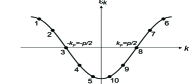
Figure 1: Discretization of the momenta in the Brillouin zone. This figure shows the case $N=10$.

Our functional RG equations for the one-dimensional EHM at one-loop follow closely the approach of Zanchi and Schulz Zanchi , which itself is an adaptation of the two-dimensional RG for fermions Shankar to the case of an arbitrary Fermi surface. This and other formulations of the functional RG have recently been applied to several two-dimensional interacting electron systems Honerkamp1 ; Halboth ; Tsai ; Binz ; Kampf . The crucial difference is that we consider a finite number $N$ of divisions of the magnitude of the momenta, while the two-dimensional calculations discretize the Fermi surface into angular patches. At one-loop level our equations become:

$$\frac{dg(k_{1},k_{2},k_{3})}{d\Lambda}=$$ (2)

$$- \!\!\!\!\int\!d\underline{p}\frac{d}{d\Lambda}[G_{\Lambda}(\underline{p})G_{\Lambda}(\underline{k})]g(k_{1},k_{2},k)g(p,k,k_{3})$$

$$- \!\!\!\!\int\!d\underline{p}\frac{d}{d\Lambda}[G_{\Lambda}(\underline{p})G_{\Lambda}(\underline{q_{1}})]g(p,k_{2},q_{1})g(k_{1},q_{1},k_{3})$$

$$- \!\!\!\!\int\!d\underline{p}\frac{d}{d\Lambda}[G_{\Lambda}(\underline{p})G_{\Lambda}(\underline{q_{2}})][-\!2g(k_{1},p,q_{2})g(q_{2},k_{2},k_{3})$$

$$+ \!\!g(p,k_{1},q_{2})g(q_{2},k_{2},k_{3})\!+\!g(k_{1},p,q_{2})g(k_{2},q_{2},\!k_{3})],$$

where $k=k_{1}+k_{2}-p$, $q_{1}=p+k_{3}-k_{1}$, $q_{2}=p+k_{3}-k_{2}$, $\underline{p}=(p,\omega)$, $\int d\underline{p}=\int dp\sum_{\omega}1/(2\pi\beta)$, and $G_{\Lambda}$ is the propagator with cutoff $\Lambda$.

The high-energy modes are integrated from the full bandwidth $\Lambda_{0}$ (both positive and negative) to $\Lambda$, towards the Fermi surface. The cutoff $\Lambda$ is parameterized by the RG parameter $\ell$ as $\Lambda=\Lambda_{0}\exp(-\ell)$. The initial condition for $g(k_{1},k_{2},k_{3})$ is given by the Fourier transform of the $U$ and $V$ interaction terms. A direct analytical solution of the functional RG equation does not seem possible, and we use numerical calculations for solving the coupled integral-differential equations. For this purpose, the Brillouin zone is divided into $N$ segments. Fig. 1 shows the discretization scheme for $N=10$.

We can follow the flows of the couplings to determine the dominant instability, but a more definitive answer is given by comparing the susceptibilities corresponding to different broken symmetry states. We consider the susceptibilities of SDW, CDW, BSDW, and BCDW in the long-wavelength limit. Their general form is

$$\chi^{\delta}_{\Lambda}(\pi\!)\!\!=\!\!\!\int\!\!\!D(1,2)f(p_{1}\!)f(p_{2}\!)\langle c_{p_{1},\sigma_{1}}^{\dagger}c_{p_{1}\!+\!\pi,\sigma_{1}}c_{p_{2}\!+\!\pi,\sigma_{2}}^{\dagger}c_{p_{2},\sigma_{2}}\!\rangle,$$ (3)

where $p_{i}$ is the momentum at energy $\xi_{i}$, $\int D(1,2)\equiv\int_{|\xi_{1}|>\Lambda}d\xi_{1}J(\xi_{1})\int_{|\xi_{2}|>\Lambda}d\xi_{2}J(\xi_{2})\sum_{\sigma_{1},\sigma_{2}}s_{\sigma_{1}}s_{\sigma_{2}}$, and $J(\xi)$ is the Jacobian for the coordinate transformation from $k$ to $\xi_{k}$. For $\delta=SDW$ and $\delta=BSDW$:$s_{\uparrow}=1,s_{\downarrow}=-1$. For $\delta=CDW$ and $\delta=BCDW$: $s_{\uparrow}=1,s_{\downarrow}=1$. For $\delta=SDW$ and $\delta=CDW$:$f(p)=1$. For $\delta=BSDW$ and $\delta=BCDW$: $f(p)=\sin(p)$. In momentum space, the difference between site and bond ordering is just in the form factor, which is s-wave for site orderings and p-wave for bond orderings.

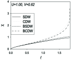
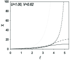
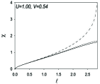
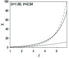
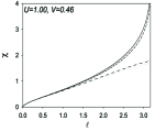
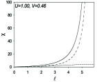
Figure 2: The flows of SDW (solid lines), CDW (dotted lines), BSDW(dashed lines), BCDW(dotted-dashed lines) susceptibilities as function of $\ell$ for $U=1$, and $V=0.46,0.54,0.62$. The left column is for $N=2$, corresponding to standard g-ology, and the right column is for $N=50$.

Under the RG procedure, the susceptibilities also flow, with the dependence on $\Lambda$ appearing both in the integration and in the flow of the expectation value $\langle...\rangle$. The dominant instability is determined by the most divergent susceptibility as $\ell$ is increased. The RG equations for the susceptibilities are,

$$\frac{d\chi^{\delta}_{\Lambda}(\pi)}{d\Lambda}\!\!\! = \!-\!\!\!\int\!\!\!d\underline{p}\frac{d}{d\Lambda}[G_{\Lambda}(\underline{p})G_{\Lambda}(\tilde{\underline{p}})](Z^{\delta}_{\Lambda}(p))^{2},$$ (4)

$$\frac{dZ^{\delta}_{\Lambda}(p)}{d\Lambda}\!\!\! = \!\!\!\!\!\int\!\!\!d\underline{p}^{\prime}\frac{d}{d\Lambda}[G_{\Lambda}(\underline{p}^{\prime})G_{\Lambda}(\tilde{\underline{p}^{\prime}})]Z^{\delta}_{\Lambda}\!(p^{\prime})g^{\delta}\!(p^{\prime}\!,p).$$ (5)

where $\tilde{\underline{p}}=\underline{p}+(\pi,0)$. For $\delta=SDW$ and $\delta=BSDW$: $g^{\delta}(p^{\prime},p)=-g(p+\pi,p^{\prime},p)$. For $\delta=CDW$ and $\delta=BCDW$: $g^{\delta}(p^{\prime},p)=2g(p^{\prime},p+\pi,p)-g(p+\pi,p^{\prime},p)$. The function $Z^{\delta}(p)$ is the effective vertex in the definition for the susceptibility $\chi^{\delta}$. Its initial condition is $1$ for SDW and CDW, and $\sin(p)$ for BSDW and BCDW. The RG equations for susceptibilities are solved with initial condition $\chi^{\delta}_{\Lambda=\Lambda_{0}}(\pi)=0$.

It is instructive to compare the difference in the susceptibility flows for the (conventional) case of two scattering points $N=2$ and for cases of multiple scattering points $N\geq 2$. We focus on the case $U=1$ (in units of $t$) which is in the weak-coupling regime ($U<\Lambda_{0}=2t$). In the left panels of Fig. 2 we show the flows of susceptibilities for $N=2$ i. e. for standard g-ology. In the right panels are results for functional RG with $N=50$. For each case, results are shown for $V=0.46,0.54$ and $0.62$. These three values were chosen to cover the SDW, BCDW and CDW phases around the $U=2V$ line.

First, we note that for $N=2$, the susceptibilities tend to diverge more quickly with $\ell$. This is because, in effect, all the renormalization corrections to the irrelevant couplings (involving radial excursions away from the Fermi points) have been assigned to the marginal ones ($g_{1}$, …, $g_{4}$ of standard g-ology). This significantly enhances the rate of increase of the couplings and of the susceptibilities. Second, for $N=2$ the SDW dominates for $V=0.46$ where $U\geq 2V$, and CDW dominates when $U\leq 2V$, as can be seen for $V=0.54$ and $0.62$. For $N=2$ all the density wave susceptibilities are degenerate at $U=2V$. Therefore, for $N=2$ there is no finite region of BCDW phase.

Importantly, for $N>2$, we find that the BCDW suscetibility is dominant in a finite range around $U=2V$. This is shown in the Fig. 2 for $N=50$, for the case $U=1,V=0.54$. For smaller (larger) $V$ the system is in the SDW (CDW) phase, as predicted by the standard g-ology. The pattern of SDW-BCDW-CDW for increasing $V$ at a fixed $U$ can be obtained by having only 6 scattering points along the band.

For our results to be reliable, it is important that they converge to a fixed result as $N$ increases. Fig. 3 shows that the phase boundaries converge quickly with $N$. Therefore, the $N=50$ results presented in Fig. 2 have reached the large $N$ limit.

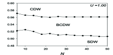
Figure 3: The shifts of the SDW-BCDW and BCDW-CDW phase boundaries with the number of momentum divisions $N$. One can note that the phase boundaries converge quickly with $N$, and they do not have any significant change for $N>30$.

The phase diagram we obtain is shown in Fig. 4. By using the momentum-dependent functional RG, we have confirmed that the BCDW phase extends to very weak coupling (at least down to $U\approx\Lambda_{0}/10$) and expands with increasing $U$. This regime is difficult to access via QMC studies, and there has also been a controversy regarding the DMRG results in this limit. Intriguing phenomena in the strong-coupling regime, such as the shrinkage of the BCDW phase can not be reliably studied by this weak-coupling FRG method. This method takes into account irrelevant terms that couple spin and charge degrees of freedom, which has been argued in Ref.Nakamura to be the cause for the disappearance of the BCDW phase at strong coupling. Nevertheless, the RG expansion is only valid for weak couplings and we focus on this limit in the present work.

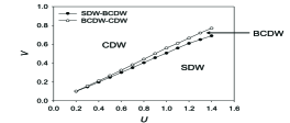
Figure 4: The phase diagram of one- dimensional EHM at half-filling in the weak coupling regime.

In summary, we have studied the phase diagram of the EHM at half-filling using a generalization of the standard g-ology to a momentum-dependent, functional RG. In conventional terms, our approach includes formally irrelevant terms corresponding to interaction vertices involving electrons at high momenta. In the present case, our procedure changes the phase diagram qualitatively because it breaks an accidental symmetry between the backscattering ($g_{1}$) and the Umklapp ($g_{3}$) processes at $U=2V$. The full momentum dependence is included in a systematic way by discretizing the momenta in the Brillouin zone into $N$ divisions. We obtain the BCDW phase near $U=2V$ by employing this consistent and well-controlled RG method at one loop level, with no additional interaction terms or ad hoc approximations. The width of this phase increases with $U$, and continues to expand until the RG procedure breaks down. We have verified that as $N$ is increased the phase boundaries become independent of the number of divisions. Our results confirm that a BCDW phase emerges spontaneously in the EHM at half-filling and clarify why this result has eluded earlier standard g-ology and bosonization techniques.

- (1) See e. g. Interacting Electrons in Reduced Dimensions, edited by D. Baeriswyl and D. K. Campbell (Plenum, New York, 1989).
- (2) T. Ishiguro and K. Yamaji, Organic Superconductors (Springer-Verlag, Berlin, 1990).
- (3) Conjugated Conducting Polymers, edited by H. G. Weiss (Springer-Verlag, Berlin, 1992).
- (4) M. Nakamura, J. Phys. Soc. Jpn. 68, 3123 (1999), Phy. Rev. B 61, 16377 (2000).
- (5) P. Sengupta, A. W. Sandvik, and D. K. Campbell, Phys. Rev. B 65, 155113 (2002), A. W. Sandvik, L. Balents, and D. K. Campbell, Phys. Rev. Lett. 92, 236401 (2004).
- (6) Y. Z. Zhang, Phys. Rev. Lett. 92, 246404 (2004).
- (7) V. J. Emery, in Highly Conducting One-Dimensional Solids, edited by J. T. Devreese, R. Evrand, and V. van Doren (Plenum, New York, 1979, p. 327.
- (8) J. Sólyom, Adv. Phys. 28, 201 (1979).
- (9) J. W. Cannon and E. Fradkin, Phys. Rev. B 41, 9435 (1990), J. W. Cannon, R. T. Scalettar, and E. Fradkin, Phys. Rev. B 44, 5995(1991).
- (10) P. G. J. van Dongen, Phys. Rev. B 49, 7904 (1994).
- (11) J. E. Hirsch, Phys. Rev. Lett. 53, 2327 (1984).
- (12) J. Voit, Phys. Rev. B 45, 4027 (1992).
- (13) E. Jeckelmann, Phys. Rev. Lett. 89, 236401 (2002) [See also a comment and reply: A. W. Sandvik, P. Sengupta, and D. K. Campbell, Phys. Rev. Lett. 91, 089701 (2003); E. Jeckelmann, Phys. Rev. Lett. 91, 089702 (2003).]
- (14) M. Tsuchiizu and A. Furusaki, Phys. Rev. Lett. 88, 056402 (2002), Phys. Rev. B 69, 035103 (2004).
- (15) For an early example stressing the subtleties that can occur in RG flows when there are accidental symmetries, see I. Affleck and J. B. Marston, J. Phys. C:Solid State Phys. 21, 2511-2526 (1988).
- (16) K. Penc and F. Mila, Phys. Rev. B 50, 11 429 (1994).
- (17) D. Zanchi and H. J. Schulz, Phys. Rev. B 54, 9509 (1996); Phys. Rev. B 61, 13609 (2000).
- (18) R. Shankar, Rev. Mod. Phys. 66, 129 (1994).
- (19) B. Binz, D. Baeriswyl, and B. Douçot, Eur. Phys. J. B 25, 69 (2002).
- (20) C. Honerkamp, M. Salmhofer, N. Furukawa, and T. M. Rice, Phys. Rev. B 63, 035109 (2001).
- (21) C. J. Halboth, W. Metzner, Phys. Rev. B 61, 7364 (2000), Phys. Rev. Lett. 85, 5162 (2000).
- (22) S. W. Tsai and J. B. Marston, Can. J. Phys. 79, 1463 (2001).
- (23) A. P. Kampf and A. A. Katanin, Phys. Rev. B 67, 125104 (2003).