Magnetic flux induced spin polarization in semiconductor multichannel rings with Rashba spin orbit coupling

Abstract

We show that a finite magnetic flux threading a multichannel semiconductor ring induces spin accumulation at the borders of the sample when the Rashba spin-orbit interaction is taken into account even in the absence of external electric fields.

In recent years semiconductor devices in which the spin orbit (SO) interaction plays a significant role, have been proposed for applications in spin controlled transport Awschalom et al. (2002). Among them, multiple connected mesoscopic geometries are natural candidates to explore how spin dependent effects manifest in the quantum interference patterns that appear in transport measurements at low temperatures Morpurgo et al (1998); nitta, meijer and takayanagi (1999). In the case of quasi-1D rings, the effect of the SO interaction has been addressed theoretically in a series of papers meir gefen and entil-wohlman (1989); loss and goldbart (1992); Balatsky and Althsuler (1993). As a consequence of the SO, the wave function acquires a non trivial spin dependent topological phase Berry (1984) that manifests in several remarkable quantum phenomena.

We will be considering SO coupling of the Rashba type which arises on a 2DEG of a semiconductor heterostructure due to the inversion asymmetry of the confining potential Bychkov and Rashba (1984). When a ring is pierced by a magnetic flux, the SO modifies the magnetic flux dependence of the spectrum and therefore the conductance Aronov and Lyanda? Geller (1993) and the persistent current (PC), in the case of an isolated ring, change as compared to the case without SO Chaplik and Magarill (1995). So far the theoretical analysis has been restricted to 1D geometries and quasi 1D in the two band approximation Splettstoesser, Governale and Zülicke (2002), where the results are qualitative the same as in the 1D systems. The multichannel nature of realistic rings employed in the experiments Mailly et al. (1993); Meijer et al. (2004) and recent controversies around the possibility of experimentally observe a spin dependent phase in transport experiments with many propagating modes Bang Yau et al. (2002); souma and Nikolic (2004) challenges us to address exactly the 2D geometry.

In this work we show that when a multichannel ring with Rashba SO coupling is pierced by a magnetic flux a spin accumulation effect is developed on the boundaries of the sample. In addition, even for an even number of electrons, a finite spin polarization in the direction perpendicular to the plane of the ring is generated whose intensity can be controlled with the magnetic flux. These phenomena share some analogies with the intrinsic Spin Hall Effect (SHE) studied in bar or T-like geometries Kato et  al. (2004); Sinova et al. (2004); Wunderlich et al. (2005), but in the present case the system is in equilibrium without external electric fields or voltage drops applied usaj and balseiro (2004).

We start by considering a 2D electron gas in the $xy$ plane confined to a mesoscopic annular region (multichannel ring) threaded by a magnetic flux $\Phi$. The single particle Hamiltonian describing an electron of effective mass $m$ subject to the Rashba SO coupling reads

$$H=\frac{{\bf p}^{2}}{2m}+V+\frac{\alpha}{\hbar}({\bf p}\times{\bf\hat{\sigma}})\cdot\hat{z}\;,$$ (1)

where $\alpha$ is the strength of the Rashba spin orbit (RSO) coupling and the Pauli matrices ${\bf\hat{\sigma}}$ are defined as standard. Employing polar coordinates $\rho$ and $\varphi$ the hard wall confining potential defining the ring is

$$V(\rho)=\left\{\begin{array}[]{l}0\;\;\mbox{for $r<\rho<R$}\\ \infty\;\;\mbox{otherwise}\;,\end{array}\right.$$ (2)

where $r$ and $R$ are the internal and external radii of the ring. The vector potential which is introduced in the Hamiltonian via the substitution, ${\bf p}=\hbar{\bf k}=-i\hbar{\bf\nabla}-\frac{e}{c}{\bf A}$, is written in the axial gauge as ${\bf A}=(\Phi/2\pi\rho)\hat{\varphi}$ . Using , $\hat{\sigma}_{\rho}=\cos\varphi\hat{\sigma}_{x}+\sin\varphi\hat{\sigma}_{y}$ and $\hat{\sigma}_{\varphi}=-\sin\varphi\hat{\sigma}_{x}+\cos\varphi\hat{\sigma}_{y}$ we can rewrite the Hamiltonian as

$$H=-\frac{\hbar^{2}}{2m}\left[\frac{1}{\rho}\partial_{\rho}\left(\rho\partial_{\rho}\right)-\frac{1}{\rho^{2}}(i\partial_{\varphi}+\nu)^{2}\right]$$

$$+i\alpha\hat{\sigma}_{\varphi}\partial_{\rho}-\frac{\alpha}{\rho}\hat{\sigma}_{\rho}\Bigl{(}i\partial_{\varphi}+\nu\Bigr{)}\,\,,$$ (3)

where $\nu=\frac{\Phi}{\Phi_{0}}$ is the magnetic flux in units of the flux quantum $\Phi_{0}={hc}{/e}$. As $J_{z}=l_{z}+s_{z}=-i\hbar\partial_{\phi}+\frac{1}{2}\hbar\hat{\sigma}_{z}$, commutes with $H$, the eigenfunctions can be chosen as

$$\psi_{j}(\rho,\varphi)=\left[\begin{array}[]{c}e^{i(l)\varphi}\tilde{f}_{l}(\rho)\\ e^{i(l+1)\varphi}\tilde{g}_{l+1}(\rho)\end{array}\right].$$ (4)

where $J_{z}\psi_{j}=\hbar j\psi_{j}$ and $j=l+\frac{1}{2}$. In what follows it will be useful to work with dimensionless variables. With that purpose we define the dimensionless coordinate $\xi=\rho/R$, the aspect ratio $\lambda=R/r$ and

$$\epsilon=\frac{2mER^{2}}{\hbar^{2}}\equiv\frac{E}{E_{0}}\,\,,\,\,\beta=2R\frac{\alpha m}{\hbar^{2}}\,\,,\,\,f_{l}=R\tilde{f}_{l}\,\,,\,\,g_{l}=R\tilde{g}_{l}\;,$$ (5)

with the boundary conditions

$$f_{l}({\lambda}^{-1})=g_{l+1}({\lambda}^{-1})=0=f_{l}(1)=g_{l+1}(1)\;.$$ (6)

We can look solutions of the form $f_{l}(\xi)\sim Y_{l-\nu}(k\xi)$ and $g_{l+1}(\xi)\sim Y_{l+1-\nu}(k\xi)$ where $Y_{l}(\xi)$ are Bessel functions of the type $J_{l}(\xi)$ or $N_{l}(\xi)$. The Rashba term simply acts as rising or lowering operator on the Bessel function basis since the following standard recurrence relations hold Abramowitz and Stegun (1972):

$$\left(\frac{d}{d\xi}+\frac{1\pm l}{\xi}\right)Y_{l\pm 1}(k\xi)=\pm kY_{l}(k\xi)\;.$$ (7)

This is indeed the property which allows to obtain, as in the case of a disk geometry TLG (2004), an exact analytical solution. Due to the RSO, the bulk spectrum has two branches

$$\epsilon=k^{2}\pm\beta k\;.$$ (8)

Therefore for a given value of $\epsilon$ there are two non-trivial solutions for the momentum $k$ that we denote $k^{+}$ and $k^{-}$ respectively. It is then possible to obtain a solution as

$$Y(\xi)=\left(f_{l}\atop g_{l+1}\right)=\sum_{i=1}^{4}c_{i}Y_{i}(\xi)=\sum_{i=1}^{4}c_{i}\left(Y_{i}^{1}\atop Y_{i}^{2}\right)$$ (9)

with

$$Y_{1}(\xi)=\left(\begin{array}[]{c}J_{l-\nu}(k^{+}\xi)\\ J_{l-\nu+1}(k^{+}\xi)\end{array}\right)\;, Y_{2}(\xi)=\left(\begin{array}[]{c}J_{l-\nu}(k^{-}\xi)\\ -\frac{|\epsilon|}{\epsilon}J_{l-\nu+1}(k^{-}\xi)\end{array}\right)$$ (14)

and with $Y_{3}$ and $Y_{4}$ obtained from $Y_{1}$ and $Y_{2}$ by exchanging Bessel functions of type $J$ by Bessel functions of type $N$.

Defining $\tilde{Y}$ as,

$$\tilde{Y}=\left(\begin{array}[]{cccc}Y_{1}^{1}({\lambda}^{-1})&Y_{2}^{1}(\lambda^{-1})&Y_{3}^{1}(\lambda^{-1})&Y_{4}^{1}(\lambda^{-1})\\ Y_{1}^{2}(\lambda^{-1})&Y_{2}^{2}(\lambda^{-1})&Y_{3}^{2}(\lambda^{-1})&Y_{4}^{2}(\lambda^{-1})\\ Y_{1}^{1}(1)&Y_{2}^{1}(1)&Y_{3}^{1}(1)&Y_{4}^{1}(1)\\ Y_{1}^{2}(1)&Y_{2}^{2}(1)&Y_{3}^{2}(1)&Y_{4}^{2}(1)\\ \end{array}\!\right),$$ (15)

the boundary conditions lead to the equation $\det(\tilde{Y})=0$. Given $\beta$, $\lambda$ and $\nu$ we solve this equation to obtain the (dimensionless) energies $\epsilon_{j,i}(\nu)$ where $j$ is the total angular momentum and $i$ labels the different eigenstates for a fixed $j$, in such a way that for $\nu=0$ and $\beta=0$ we have $\epsilon_{j,i}<\epsilon_{j,i+1}$.

In order to fix numerical estimates for the parameters we consider characteristic values extracted from recent experiments performed on semiconductor heterostructures defined on a 2DEG. Rings with external radius $R\sim 400-500nm$ and an aspect ratio $\lambda\sim 2$ have been recently employed as devices Meijer et al. (2004). Typical values for the Fermi wavelength are $\lambda_{F}\sim 40-50nm$ that give $k_{F}\sim 0.1nm^{-1}$. For $R=400nm$ one gets a maximum value of the (dimensionless) Fermi energy $\epsilon_{F}=(Rk_{F})^{2}\sim 1600$. For an effective mass $m\sim 0.042m_{e}$, a Rashba coupling constant $\alpha=8meVnm$ and $R\sim 400$ we obtain $\beta=2000\;nm/R(nm)\sim 4$. These parameters define the sample S studied in the present work. As the relevant situation for an isolated system, we work in the canonical ensemble keeping fixed the total number of electrons $N$ as the magnetic flux is varied. One can estimate $N$ at zero flux Baltes et al. (1976), that in this case gives $N=[3\;\epsilon_{F}/8]=600$ (the symbol $[..]$ denotes integer part). The maximum number of transverse channels $M$ can be then calculated as Fendrik and Sánchez (2000)

$$M=\big{[}\frac{2\sqrt{N}(\lambda-1)}{\pi\sqrt{\lambda^{2}-1}}\big{]}\;.$$ (16)

Thus for $N\sim 200-600$ one gets $M\sim 4-8$, in agreement with the reported experimental values Mailly et al. (1993).

For $\nu=0$ and finite $\beta$, the SO breaks the degeneracy between states differing in one unit of $j$. The degeneracy between states with opposite values of $j$ is broken by the presence of a finite magnetic flux $\nu$, being the charge PC the signature of this broken symmetry.

As discussed previously in the literature, in $1D$ rings the RSO induces a topological phase Aronov and Lyanda? Geller (1993), $\Delta_{B}=\frac{\alpha\;m}{\hbar^{2}}\oint(\hat{z}\times\sigma)\cdot d\mathbf{l}$, that once added to the Bohm-Aharonov one, $2\pi\nu$, leads to an ”effective flux” $\nu_{eff}=\nu+\frac{1}{2}(1\mp\sqrt{(2\alpha\;ma/\hbar^{2})+1})$ (the $\pm$ sign depends on the sign of the $z$ spin projection in the local spin frame and $a$ is the radius of the ring). It is then via this effective flux that the SO interaction affects the behavior of the PC Chaplik and Magarill (1995).

The situation in the 2-D ring is considerably more involved. We display in Fig.1 some regions of the spectrum for both $\beta=0$ and $\beta=4$ cases. The upper panel of Fig.1 shows the lowest eigenvalues of the multichannel ring S as a function of $\nu$. As the first transverse channel is active in that region, the spectrum is similar to that of the $1D$ ring (due to the symmetry respect to $\nu=0.5$ the spectrum is shown for $0\leq\nu\leq 0.5$). We can observe the evolution with $\nu$ of the single particle energy states labeled by the quantum numbers $(j,i)$. For $\beta=0$ (bold dotted lines) we have the double degenerate fundamental states, $(\pm 1/2,0)$, and the doublets $(1/2,1),(3/2,0)$ and $(-1/2,1),(-3/2,0)$. Notice that at $\nu=0$, except the fundamental state, the others are four-fold degenerate and, as in the $1D$ regime, crossings occur only at $\nu=0,0.5$. The effect of a finite RSO coupling is clearly visible in the figure. The RSO interaction lowers the energy of each state and it can even change the order in which they appear. For the case shown in Fig.1, the lowest energy states are $(3/2,0)$ and $(-3/2,0)$ that for finite flux remain almost degenerate and appear in the figure as a single line. We then have four states which for very small $\nu$ (i.e, before any $\nu$ induced level crossing) are ordered as $(-1/2,0)$, $(1/2,0)$, $(5/2,0)$, $(-5/2,0)$. Higher in energy, we display the states $(1/2,1)$, $(-1/2,1)$, $(-7/2,0)$, $(7/2,0)$. Notice that as a result of the RSO new crossings appear. As an example, we draw arrows in the panel as guides for the location of the new crossings between $(1/2,0)$ and $(5/2,0)$ and $(-1/2,1)$, $(-7/2,0)$. These crossings are indeed the fingerprints of the effective flux $\nu_{eff}$ mentioned above note .

When many transverse channels are activated the spectrum displays additional crossings between levels belonging to different channels, even in the absence of RSO coupling (see lower panel of Fig.1). The crossings that arise due to the SO interaction are mixed with the crossings between levels with different transverse channel number and it is not straightforward to identify the signature of an effective flux like in the 1D case, when only a single transverse channel is active. This can be understood looking at the functional form of the 2D Hamiltonian Eq.(Magnetic flux induced spin polarization in semiconductor multichannel rings with Rashba spin orbit coupling), whose last term contains the ratio $\alpha/\rho$ between the RSO constant and the radial coordinate. Therefore, loosely speaking, on average each transverse channel feels a topological phase that depends on the value of the transverse quantum number. This argument could be extended to explain the difference in patterns of conductance oscillations of single-channel and multichannel open rings with RSO interaction souma and Nikolic (2004).

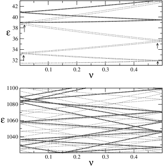
Figure 1: Dimensionless energies $\epsilon$ as a function of the magnetic flux $\nu$ for the annular cavity $\bf{S}$ defined in the text. Upper panel: lowest eigenvalues in the absence of RSO (bold dotted lines) and for $\beta=4$ (small dotted lines). The arrows are guides for the eyes to locate the position of the crossings due to the RSO coupling. See the text for details. Lower panel: high energy region showing many crossings between different transverse channels, in the absence of RSO (bold dotted lines) and for $\beta=4$ (small dotted lines).

In terms of the dimensionless variables, the only non vanishing component of the charge current density for eigenstates as given in Eq.(4) reads,

$$J_{\varphi}=\frac{e\hbar}{mR^{3}\xi}\left((l-\nu)f_{l}^{2}+(l+1-\nu)g_{l+1}^{2}+\beta\;\xi\;f_{l}\;g_{l+1}\right)\;.$$ (17)

Employing the probability and spin densities, $\delta_{j}(\xi)\equiv f_{l}^{2}+g_{l+1}^{2}$, $\langle\hat{\sigma}_{z}\rangle_{j}\equiv\Psi^{\dagger}\hat{\sigma}_{z}\Psi$ and $\langle\hat{\sigma}_{\rho}\rangle_{j}\equiv\Psi^{\dagger}\hat{\sigma}_{\rho}\Psi$, the current can be written as

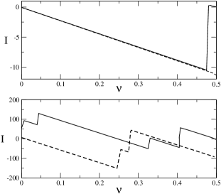
Figure 2: Persistent current $I$ as a function of $\nu$ in the absence of SO interaction (dashed lines) and for $\beta=4$ (solid line). Upper panel corresponds to $N=6$ and lower panel to $N=182$. The finite slope of the jumps is due to size of the flux step ($5.10^{-}3$ ) employed in the numerical calculations

$$J_{\varphi}=\frac{e\hbar}{mR^{3}\xi}\left((j-\nu)\delta_{j}(\xi)-\frac{1}{2}\langle\hat{\sigma}_{z}\rangle_{j}+\frac{\beta}{2}\;\langle\hat{\sigma}_{\rho}\rangle_{j}\;\xi\right)\;.$$ (18)

Therefore the effect of the SO interaction in the charge current density is unveiled in the last term of Eq.(18). To calculate the total charge PC we have to sum the contributions of all states up to the Fermi energy,

$$\tilde{I}=\int_{r}^{R}d\rho\sum J_{\varphi}^{(n)}(\rho)=-c\frac{\partial E}{\partial\phi}$$ (19)

where as before, $n$ labels the occupied states. Besides a geometrical factor that takes into account the area of the outer circle of the sample $\tilde{I}$ is the magnetic moment. In terms of the dimensionless variables,

$$\tilde{I}=\frac{cE_{0}}{\phi_{0}}I\,,\,\,\,I=-\frac{\partial\epsilon}{\partial\nu}\;,$$ (20)

For the parameters quoted before for sample $\bf S$, results $\tilde{I}\sim 0.2\;I(nA)$. In Fig.2 we plot $I$ as a function of $\nu$ for $N=6(M=1)$ and $N=182(M=4)$ in order to show how active open channels modify the behavior of the PC and the determination of an effective flux as in the $1D$ regime note2 .

As a result of the RSO interaction, spin projection is not a good quantum number. For N occupied states, the mean value of the z-projection of the spin is proportional to

$$\Sigma_{z}=\int_{ring}\sum_{n}\Psi_{n}^{\dagger}\hat{\sigma}_{z}\Psi_{n}=2\pi\int_{\frac{1}{\lambda}}^{1}\sigma_{z}(\xi)\xi d\xi$$ (21)

where $n=1,N(\epsilon_{F})$ labels the occupied states and $\sigma_{z}(\xi)$ corresponds to the total spin density for N particles. Even in the case of N even, a non zero spin density is obtained when SO is present and $\nu\neq 0$. In addition a spin accumulation effect is developed and it is manifested in the tendency of $\sigma_{z}$ to be positive on one border of the sample and negative on the other one. Although the accumulation becomes stronger as N and the number of open channels increase, it is also present when only one transverse channel is active. In order to explain the origin of the effect we first concentrate in a pair of eigenstates that, being degenerate at $\nu=0$ with opposite value of $j$ and with opposite out of plane spin projection, become non-degenerated for finite $\nu$. The expectation value of $\hat{\sigma}_{z}$ in a given $\Psi_{j}$ is $\langle\hat{\sigma}_{z}\rangle_{j}=|{f}_{l-\nu}|^{2}-|{g}_{l-\nu+1}|^{2}$. It is straightforward to verify that at $\nu=0$ states with opposite value of $j$ have opposite value of $\langle\hat{\sigma}_{z}\rangle$ and therefore for even number of particles $N=2p$ , is ${\sigma}_{z}(\xi)=0$. As $\nu>0$, two facts induce a spin accumulation effect. On one hand, the magnetic field breaks the symmetry between single particle states with opposite value of $j$ and on the other hand, due to the presence of additional level crossings the total $J_{z}$ of the ground state can change and be different from zero for finite flux.

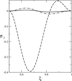
Figure 3: Dimensionless total spin density $\sigma_{z}$ as a function of $\xi$ for $\nu=0.2$ for the sample $\bf{S}$. $N=2$ (solid line), $N=4$ (dashed line) and $N=6$ (dotted-dashed line).

In Fig. 3, we show $\sigma_{z}$ for $\beta=4$, $\nu=0.2$ and $N=2,4,6$. For $N=2$, the single particle states have $j=\pm 3/2$. As $\nu$ is turned on, the effective orbital index $l_{eff}\equiv l-\nu$ becomes $1-\nu$ and $-2-\nu$ for $j=3/2$ and $j=-3/2$ respectively. Thus as the modulus of the effective orbital index decreases (increases) for $j=3/2$ ($j=-3/2$), the probability density and $<\hat{\sigma}_{z}>_{j(-j)}$ are pushed toward the internal (external) boundary of the sample. This symmetry breaking explains the observed accumulation effect in this case. For $N=4$ the situation is different. Due to the level crossing mentioned before, the single particle states in the ground state have $j=3/2,-3/2,-1/2,5/2$ and the accumulation effect is mainly due to the unbalance between the last two states. We show the case $N=6$ which again is similar to the case $N=2$.

As the particle number is increased to the relevant experimental values, transverse channels are activated and the description of the effect becomes more complicated. Nevertheless our simulations suggest that the accumulations effect is a generic feature of the system in the presence of a magnetic flux. As an illustration, in Fig. 4 we show the spin density $\sigma_{z}$ as a function of the dimensionless coordinate $\xi$ for $N=181$ and $N=182$ and different values of the magnetic flux in the range $0<\nu<0.5$. For $N=181$ and $\nu=0$ (see Fig.4 a)) a finite $\sigma_{z}(\xi)$ is obtained which value corresponds to the last occupied level, as expected for odd particle number. On the other hand, for $N=182$ is $\sigma_{z}(\xi)=0$ at $\nu=0$, as it is shown in Fig.4 b). For $\nu>0$ the spin density profile has a more complicated structure than in the quasi 1D regime due to the behavior of the radial components of the spinors as the number of transverse channels increases and the flux is varied.

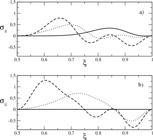
Figure 4: Dimensionless total spin density $\sigma_{z}$ as a function of $\xi$ for $\nu=0$ (solid line) , $\nu=0.1$ (dotted line) and $\nu=0.45$ (dashed line) for the sample $\bf{S}$. a) $N=181$, b) $N=182$. Note that in this case is $\sigma_{z}=0$ for $\nu=0$ as expected for an even number of particles.

In summary we have shown that a finite magnetic flux threading a multichannel semiconductor ring with SO interaction induces spin polarization with opposite sign for the two borders of the ring. We believe this system constitutes a new proposal to detect accumulation effects induce by SO interaction in constrain geometries in equilibrium, that is without applied electric fields or currents. The characteristic wavelength of the accumulation effect is of the order of $.1\mu m$, which is not far from the sensitivity of methods employed recently to probe spin polarization in semiconductor channels Kato et  al. (2004). Besides the accumulation effect, the integrated spin density $\Sigma_{z}$ is different from zero and is sensitive to the value of the magnetic flux, as can be inferred from Fig.4. In the presence of an external magnetic field perturbation, the spin magnetization should be proportional to $\Sigma_{z}$. With the help of new experimental techniques based on resonant methods it should be possible to sense changes in the total magnetization of isolated rings due to SO interaction R. Deblock, R. Bel, B. Reulet, H. Bouchiat, D. Mailly (2002).

Partial financial support by ANPCyT Grant 03-11609, CONICET and Foundación Antorchas Grant 14248/113 are gratefully acknowledged. We would like to thank C. Balseiro and G. Usaj for helpful discussions. G.S.L thanks ICTP, Trieste, where part of this work was done.

References

- Awschalom et al. (2002) D. Awschalom, N. Samarth, and D. Loss, eds., Semiconductor Spintronics and Quantum Computation (Springer, New York, 2002).
- Morpurgo et al (1998) A. F Morpurgo, J. P Heida, T.M Klapwijk and B.J van Wees,Phys. Rev. Lett. 80, 1050 (1998).
- nitta, meijer and takayanagi (1999) J. Nitta, F.E Meijer and H. Takayanagi, Appl. Phys. Lett. 75, 695 (1999).
- meir gefen and entil-wohlman (1989) Y. Meir, Y. Gefen and O. Entil-Wohlman, Phys. Rev. Lett. 63, 798 (1989).
- loss and goldbart (1992) D. Loss and P. M. Goldbart, Phys. Rev. B. 45, 13544 (1992).
- Balatsky and Althsuler (1993) A. V. Balatsky and B. L. Althsuler, Phys. Rev. Lett. 70, 1678 (1993).
- Berry (1984) M. V. Berry, Proc. R. Soc. London A 392, 45 (1984).
- Bychkov and Rashba (1984) Y. A. Bychkov and E. I. Rashba, JETP Letters 39, 78 (1984).
- Aronov and Lyanda? Geller (1993) A. G. Aronov and Y. B. Lyanda–Geller, Phys. Rev. Lett. 70, 343 (1993).
- Chaplik and Magarill (1995) A. V. Chaplik and L. I. MaGarill, Superlattices and Microstructures 18, 321 (1995).
- Splettstoesser, Governale and Zülicke (2002) J. Splettstoesser, M. Governale and U. Zülicke, Phys. Rev. B 68, 165341 (2003).
- Mailly et al. (1993) D. Mailly, C. Chapelier and A. Benoit, Phys. Rev. Lett. 70, 2020 (1993).
- Meijer et al. (2004) F. Meijer, A. Morpurgo, T. Klapwijk, T. Koga, and J. Nitta,Phys. Rev. B. 69, 035308 (2004).
- Bang Yau et al. (2002) Jeng-Bang Yau, E. P De Poortere and M. Shayegan, Phys. Rev. Lett. 88, 146801 (2002).
- souma and Nikolic (2004) S. Souma and B. K. Nikolíc, Phys. Rev. B. 70, 195346 (2004).
- Kato et al. (2004) Y.K Kato, R.C Myers, A.C Gossard and D.D Awschalom, Science 306, 1910 (2004).
- Sinova et al. (2004) J. Sinova, D. Culcer, Q. Niu, N. A. Sinitsyn, T. Jungwirth and A. H.MacDonald, Phys. Rev. Lett. 92, 126603 (2004).
- Wunderlich et al. (2005) J. Wunderlich, B. Kaestner, J. Sinova and T. Jungwirth, Phys. Rev. Lett. 94, 047204 (2005).
- usaj and balseiro (2004) G. Usaj and C.A Balseiro, cond-mat/0405065.
- Abramowitz and Stegun (1972) M. Abramowitz and I.A. Stegun, Handbook of Mathematical Functions, (Dover, New York, 1972).
- TLG (2004) E. Tsitsishvili, G. S. Lozano and A. O. Gogolin, Phys. Rev. B 70, 115316 (2004).
- Baltes et al. (1976) M. Baltes and E. Hilf, Spectra of finite systems, (Bibliographisches Institut, Mannheim, 1976).
- Fendrik and Sánchez (2000) A.J. Fendrik and M.J Sánchez, Eur. Phys. J. B 14, 725 (2000).
- (24) Assuming a ring of radius and employing the dispersion relation for 1D geometries Aronov and Lyanda? Geller (1993), it is straightforward to obtain the values of , given two levels with and for example.
- (25) In order to decrease CPU time in the numerical simulations, and without loss of generality, we employ for the present analysis these values of . Although they are smaller that the ones that correspond to the experimental reported , the results and conclusions are completely general, as many transverse channels are open.
- R. Deblock, R. Bel, B. Reulet, H. Bouchiat, D. Mailly (2002) R. Deblock, R. Bel, B. Reulet, H. Bouchiat and D. Mailly, Phys. Rev. Lett. 89, 206803 (2002).