Energy Down Conversion between Classical Electromagnetic Fields via a Quantum Mechanical SQUID Ring

Abstract

We consider the interaction of a quantum mechanical SQUID ring with a classical resonator (a parallel $LC$ tank circuit). In our model we assume that the evolution of the ring maintains its quantum mechanical nature, even though the circuit to which it is coupled is treated classically. We show that when the SQUID ring is driven by a classical monochromatic microwave source, energy can be transferred between this input and the tank circuit, even when the frequency ratio between them is very large. Essentially, these calculations deal with the coupling between a single macroscopic quantum object (the SQUID ring) and a classical circuit measurement device where due account is taken of the non-perturbative behaviour of the ring and the concomitant non-linear interaction of the ring with this device.

I
Introduction

With the now very serious interest being taken in the possibilities of creating quantum technologies such as quantum information processing and quantum computing r1 ; r2 ; r3 , much attention is being focused on the application of Josephson effect devices, particularly the SQUID ring. As has been demonstrated recently, with the appropriate ring circuit parameters and operating temperature these devices can display manifestly macroscopic quantum behaviour such as macroscopically distinct superposition of states r4 ; r5 ; r6 ; r7 ; r8 ; r9 ; r10 ; r11 . In any considerations of quantum technologies the role of the environment, as coupled to the quantum object, has featured very strongly r12 ; r13 ; r14 . With regard to using superconducting systems in quantum technologies, it has been shown that Josephson weak link circuits, and in particular SQUID rings in the quantum regime, are highly non-perturbative in nature and can generate very strong non-linear interactions with classical circuit environments r15 . In this paper we provided a demonstration that this non-perturbative (non-linear) behaviour is crucial to the understanding of the interaction of SQUID rings with circuit environments. In this work we first consider the adiabatic (ground state) interaction of a quantum regime SQUID ring inductively coupled to a classical parallel resonance $LC$ (tank) circuit.

Figure 1: (a) Schematic of a (quantum regime) SQUID ring inductively coupled to a driven tank circuit (two mode system) (b) schematic of a three mode system: classical input microwave excitation source - SQUID ring - and an inductively coupled tank circuit.

This circuit system is shown schematically in figure 1(a). We then continue to consider energy transfer between a classical monochromatic microwave source (the input) and this classical electromagnetic (em) field mode (the output) via the quantum mechanical SQUID ring (figure 1(b)). Here, as in other work r16 , we have modelled this output mode as a parallel $LC$ equivalent circuit. However, in this paper we have treated this circuit environment as classical since we wish to explore a region of the system parameter space, involving large input-output frequency ratios, which is of current experimental significance. When treated fully quantum mechanically, such simulations are beyond the reach of the computing power available to us. As the essential result of this paper, we show that the non-perturbative (non-linear) interaction generated by the SQUID ring is made manifest through energy conversion between the input and output, even if these differ greatly in frequency. In part this has been inspired by past experimental results where we have demonstrated r17 that very high ratio frequency down conversion can occur between a microwave source and a radio frequency $\left(\approx 20\mathrm{MHz}\right)$ tank circuit via the intermediary of a very small capacitance SQUID ring r17 . In these previous results we recorded a frequency down conversion ratio of 500:1. In recent, as yet to be published data, this has been improved upon by refinements in electronic technique to yield a ratio as high as 6,500:1 between a a few GHz microwave input field and a sub-MHz tank circuit. We know of no classical non-linear circuit device that could generate such large ratios laser and, given the very small capacitance (niobium point contact) SQUID rings we were using in our experiments, it was clearly of interest to see whether a quantum regime SQUID ring could lead to this massive frequency down conversion. In a recent publication r18 we considered this problem in the context of the persistent current qubit circuit model introduced by Orlando et al r19 , where this quantum element acted as the medium for coupling two classical field environments together. Specifically, the qubit was driven by a classical electromagnetic (em) field (the input) which was used to pump the qubit into an excited state. To deal with energy conversion to an dissipative output em mode, a quantum jumps approach was adopted to model the decay of the excited qubit with the energy dumped into this mode. Using this approach we were able to demonstrate small ratio (500MHz to 300MHz) frequency down conversion from input to output through the intermediary of the quantum qubit loop. In this work, with a single weak link SQUID ring as the quantum intermediary, we adopt a less complicated model, where the SQUID ring simply follows Schrödinger evolution without the introduction of quantum jumps. We then show, to the limits of the computational power available to us, that a two orders of magnitude frequency down conversion (from microwave to radio frequencies) is possible. In doing so we also demonstrate that the interaction between a quantum mechanical SQUID ring and its classical circuit environment is in no way trivial and requires a detailed understanding of the non-perturbative properties of SQUID rings. We emphasise that with this result established, and without any other obvious physical constraints, it seems reasonable to assume from a theoretical viewpoint that even higher ratio frequency down conversion could be realised if the necessary computational power were available. At present, apart from essentially fixed frequency masers, sources of quantum mechanical em fields at microwave frequencies are not readily available. Thus, given the non-perturbative properties of SQUID rings in the quantum regime, it also seems reasonable to consider how such devices could make manifest their quantum mechanical nature through the interaction with classical em fields and field oscillator modes.

In the well known lumped component model of a quantum mechanical SQUID ring (in this work one Josephson weak link device, of effective capacitance $C_{s}$, enclosed by a thick superconducting ring of inductance $\Lambda_{s}$, with a classical magnetic flux of $\Phi_{x}$ applied to the ring) the Hamiltonian for the ring is given by r20 ; r21

$$H_{s}=\frac{\hat{Q}_{s}^{2}}{2C_{s}}+\frac{\left(\hat{\Phi}_{s}-\Phi_{x}\right)^{2}}{2\Lambda_{s}}-\hbar\nu\cos\left(\frac{2\pi\hat{\Phi}_{s}}{\Phi_{0}}\right)$$ (1)

where, with a circumflex denoting operators, $\hat{\Phi}_{s}$ (the magnetic flux threading the ring of the SQUID device) and $\hat{Q}_{s}$ (the Maxwell electric displacement flux between the electrodes of the weak link) are canonically conjugate quantum variables such that $\left[\hat{\Phi}_{s},\hat{Q}_{s}\right]=i\hbar$ with $\hat{Q}_{s}\rightarrow-i\hbar\partial/\partial\Phi_{s}$ and $\Delta\hat{\Phi}_{s}\Delta\hat{Q}_{s}\geq\hbar/2$. Here, the third term on the right hand side of (1) is due to the Josephson phase coherent coupling energy, with matrix element $\hbar\nu/2$, arising from the weak link critical current $I_{c}=2e\nu$, with periodicity set by the superconducting flux quantum $\Phi_{0}=h/2e$. We assume that the ambient temperature $\left(T\right)$ of the SQUID is such that $\hbar\omega_{s}\gg k_{B}T$ for a characteristic ring oscillator frequency of $\omega_{s}/2\pi\left(=1/2\pi\sqrt{\Lambda_{s}C_{s}}\right)$. Operating in this quantum regime the time independent Schrödinger equation (TISE) for the SQUID ring then reads

$$\left[\frac{\hat{Q}_{s}^{2}}{2C}+\frac{\left(\hat{\Phi}_{s}-\Phi_{x}\right)^{2}}{2\Lambda}-\hbar\nu\cos\left(\frac{2\pi\hat{\Phi}_{s}}{\Phi_{0}}\right)\right]\left|\psi_{\kappa}\right\rangle=E_{\kappa}\left|\psi_{\kappa}\right\rangle$$ (2)

for ring eigenfunctions $\left|\psi_{\kappa}\right\rangle$($\kappa=0$ the ground state, $\kappa=1$ the first excited state, etc.) and ring eigenenergies $E_{\kappa}$ (as shown in figure 2), these eigenenergies being $\Phi_{0}$-periodic in the external magnetic flux applied to the ring.

Figure 2: Plot of the eigenenergies of the SQUID ring Hamiltonian, found by solving the TISE, as a function of external applied flux with $\hbar\omega_{s}=0.006\Phi_{0}^{2}/\Lambda_{s}$ and $\hbar\nu=0.035\Phi_{0}^{2}/\Lambda_{s}$

II Dynamics of a Coupled Quantum SQUID Ring-Classical Resonator System

II.1 Adiabatic Regime

In the time independent (adiabatic) case the experimentally accessible state is the ground state $\left(\kappa=0\right)$ for which the expectation value of the screening supercurrent flowing around the ring is $\langle\hat{I}_{s}\left(\Phi_{x}\right)\rangle=-\left\langle\partial\hat{H}/\partial\Phi_{x}\right\rangle=\left\langle\left(\hat{\Phi}_{s}-\Phi_{x}\right)/\Lambda_{s}\right\rangle$ r17 ; r20 . For relatively large values of $\hbar\nu$ (and hence $I_{c}$) this ground state screening current takes the form of a rounded sawtooth centred on $\Phi_{x}=\Phi_{0}/2$ (modulo $n\Phi_{0}$, $n$ integer). Thus, the ring screening current is clearly a highly non-linear function of $\Phi_{x}$, as is its magnetic susceptibility $\chi_{s}=\partial\langle\hat{I}_{s}\left(\Phi_{x}\right)\rangle/\partial\Phi_{x}$. At $\Phi_{x}=\left(n+1/2\right)\Phi_{0}$, $n$ integer, the ring is in an quantum superposition, with equal coefficients, of clockwise and anti-clockwise screening currents (equivalently flux states). A rounded sawtooth jump in the screening current, centred at half integer bias flux, correspondingly generates a narrow positive spike in $\chi_{s}\left(\Phi_{x}\right)$ at this flux value. At integer bias flux $\left(\Phi_{x}=n\Phi_{0}\right)$ the susceptibility is a minimum, increasing monotonically to a maximum at $\Phi_{x}=\left(n+1/2\right)\Phi_{0}$. As we have shown, in this simple ground state model of a quantum regime SQUID ring the evolution of its quantum state can be monitored through its effect on the classical dynamics of a measurement circuit coupled to it r15 ; r17 ; r20 . Typically this takes the form of a low frequency, parallel $LC$ tank circuit inductively coupled to the SQUID ring and excited at, or very close to, its resonant frequency. The resonant frequency of this tank circuit $\left(\omega_{t}/2\pi\right)$ is usually extremely low compared with the natural oscillator frequency of the SQUID ring (with the implicit assumption that $\hbar\omega_{t}\ll k_{B}T$). This configuration is very well known and forms the basis for one type of ultra sensitive magnetic flux detector - the ac or radio frequency biased SQUID magnetometer r21 . With this tank circuit playing the role of the classical measurement system for the SQUID ring, a changing $\chi_{s}\left(\Phi_{x}\right)$ leads, in the ground state of the ring, to downward shifts (due to the positive $\chi_{s}\left(\Phi_{x}\right)$) of the resonant frequency of the tank circuit. For this ground state, therefore, following the change in the frequency (and amplitude) of the tank circuit resonance allows us to extract some information concerning the evolution of the quantum state of the ring (i.e. the coefficients in its screening current superposition) as a function of $\Phi_{x}$.

II.2 The Born-Oppenheimer Approximation

Given that the oscillator frequencies of both the SQUID ring and the (classical) tank circuit resonator are functions of their circuit capacitances, it is, in this limit, often convenient to introduce an approach well known in atomic physics. These capacitances can be considered as measures of the effective mass of each circuit (SQUID ring and tank circuit resonator). Crucially, for quantum regime SQUID rings these capacitances (effective masses) will be markedly different in magnitude, e.g. for the ring typically $\approx$ a few $\times 10^{-15}\mathrm{F}$ and for the tank circuit $\approx$ a few $\times 10^{-11}\mathrm{F}$, or more. This low mass-high mass (here, low capacitance-high capacitance) situation was dealt with many years ago by Born and Oppenheimer for nuclear-electron motion. Adopting this approach we compute from solutions of (2) the expectation value of the screening supercurrent in the SQUID ring (fast) and substitute this as a feedback term into the classical equation of motion for the tank circuit (slow). Provided that the resonant frequency of the tank circuit is low enough, so that to an extremely good approximation the quantum SQUID ring remains adiabatically in its ground state, the equation of motion for the coupled ring-tank circuit system then reads r15 ; r20

$$C_{t}\frac{\partial^{2}\Phi_{t}}{\partial t^{2}}+\frac{1}{R_{t}}\frac{\partial\Phi_{t}}{\partial t}+\frac{1}{L_{t}}\Phi_{t}=I_{\mathrm{in}}\left(t\right)+\mu\left\langle\psi\left|\hat{I}_{s}\right|\psi\right\rangle$$ (3)

where $L_{t}$ and $C_{t}$ are, respectively, the tank circuit inductance and capacitance, $\Phi_{t}$ is the magnetic flux in the tank circuit inductor and $R_{t}$ is the resistance of the tank circuit on resonance. In this Born-Oppenheimer approximation we assume that the ring remains in one of its instantaneous energy eigenstates, i.e. solutions of (2); in reality this means the lowest energy state (the adiabatic limit). As we have demonstrated in the literature r22 , this approximation holds very well if the frequency of the drive is very small indeed compared with any separations, in frequency, between the SQUID ring energy levels. This certainly appears to be the case for radio frequency (rf) circuits, typically used to probe single weak link SQUID rings, as well as in their application in SQUID magnetometry r23 ; r24 . We note that since the SQUID ring is macroscopic in nature (as, of course, is the tank circuit) there exists a significant back reaction between these two circuits, as evidenced by the $\mu\left\langle\psi\left|\hat{I}_{s}\right|\psi\right\rangle$ term in (3). In practise this means that the SQUID ring (through the cosine in its Hamiltonian) generates a non-linear dynamic in the classical circuit environment to which it is coupled, in this case a tank circuit. For small tank circuit drive amplitudes this manifests itself as a frequency shift in the power spectrum of the tank circuit as shown in figure 3

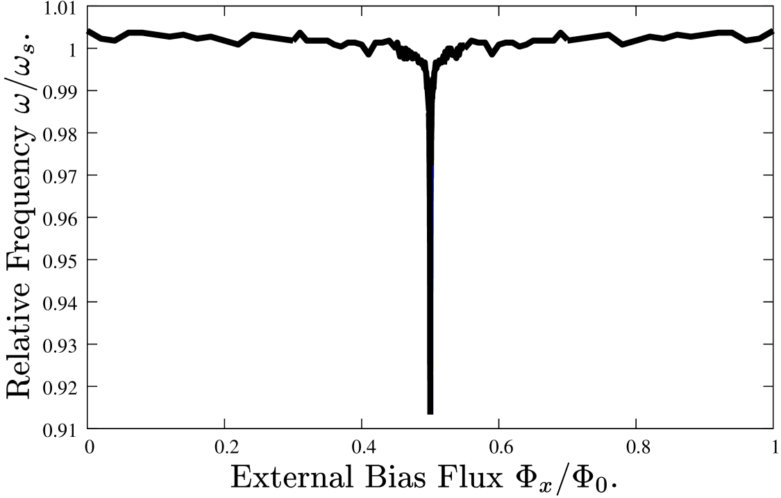
Figure 3: Frequency shift of a 130MHz tank circuit ($L_{tc}=3\times 10^{-8}H$, $C_{tc}=5\times 10^{-11}F$), coupled to the SQUID ring of figure 2, as a function of external applied flux for the ring in its ground state only (figure 2(a)) calculated using the the Born-Oppenheimer (adiabatic) approach.

III Time Dependent Schrödinger Equation Description - Exchange Regions

Following on from the time independent Schrödinger description of a SQUID ring (2), the time dependent Schrödinger equation (TDSE) for the ring takes the form

$$\left[\frac{\hat{Q}_{s}^{2}}{2C_{s}}+\frac{\left(\hat{\Phi}_{s}-\Phi_{x}\right)^{2}}{2\Lambda_{s}}-\hbar\nu\cos\left(\frac{2\pi\hat{\Phi}_{s}}{\Phi_{0}}\right)\right]\left|\psi\right\rangle=i\hbar\frac{\partial\left|\psi\right\rangle}{\partial t}$$ (4)

where $\Phi_{x}=\Phi_{x}^{\mathrm{stat}}+\Phi\left(t\right)$ is now comprises of a time dependent magnetic flux $\Phi\left(t\right)$ together with a static component $\Phi_{x}^{\mathrm{stat}}$. The intrinsically extremely non-perturbative quantum nature of the SQUID ring would indicate that the application of em fields low in frequency compared with the frequency difference $\left(\times h\right)$ between adjacent energy levels in the ring should still induce transitions between its quantum levels r25 . Thus for level differences of a few hundred GHz (quite typical of quantum regime SQUID rings), we expect em fields at microwave frequencies (a few GHz) to induce transitions, provided the field amplitude is high enough r25 . As our example in this work we consider a SQUID ring with circuit parameters commensurate with operation in the quantum regimer2 ; r26 . For this we choose $C_{s}=5\times 10^{-15}\mathrm{F}$, $\Lambda_{s}=3\times 10^{-10}\mathrm{H}$ and $\hbar\nu=0.035\Phi_{0}^{2}/\Lambda_{s}$, the latter yielding a weak link critical current $I_{c}\left(=2e\nu\right)$ of $2\mathrm{\mu A}$. Furthermore, for an oxide insulator, tunnel junction weak link (oxide thickness $\approx$ 1nm, oxide dielectric constant $\approx$ 10) in the SQUID ring, this capacitance corresponds to junction dimensions $0.25\mu m$ square, well within the capabilities of modern microfabrication technology. In turn, these dimensions imply a maximum supercurrent density in the weak link of around $4\mathrm{kAcm}^{-2}$, a perfectly reasonable value for current experiments on quantum regime SQUID rings. The SQUID ring circuit parameters $C_{s}=5\times 10^{-15}\mathrm{F}$ and $\Lambda_{s}=3\times 10^{-10}\mathrm{H}$ lead to a ring oscillator frequency $\omega_{s}/2\pi=130\mathrm{GHz}$. If we assume that the (planar) SQUID ring is fabricated in niobium, which is often the case, then this ring oscillator frequency is small compared with the superconducting energy gap in this material $\left(\approx 1000\mathrm{GHz}\right)$ at low reduced temperatures $T/T_{c}$, where $T_{c}$ is the superconducting critical temperature ($9.2K$ for niobium) for an operating (ambient) temperature in experiment typically around $40$mK.

Using the ring circuit parameters given above we showed in

Figure 4: Time averaged energy expectation values of the ring in the presence of a microwave source (input) at a frequency of 13GHz using the first two energy eigenstates as initial conditions.

figure 2 the lowest few energy eigenvalues of the SQUID ring Hamiltonian, found by solving the TISE (4), as a function of the static applied magnetic flux $\Phi_{x}^{\mathrm{stat}}$. Although such solutions of the TISE may be adequate for modelling this system if the em fields frequencies are extremely small compared with frequencies $\left(\times h\right)$ separating the ring energy levels (i.e. in the Born-Oppenheimer approximation, above), in general we must solve the TDSE where time dependent fields are involved. This is clearly demonstrated in figure 4. Here, using the the ring parameters of figure 2, we display the time averaged energy expectation values of the TDSE (4) as a function of $\Phi_{x}^{\mathrm{stat}}$, for an applied microwave field of frequency $13$GHz, amplitude $0.001\Phi_{\emph{0}}$ and using the first two eigenstates of the Hamiltonian as initial conditions. As can be seen, for this microwave frequency and amplitude there is significant energy exchange between these time averaged energies which takes place over a a very narrow range of the bias flux $\Phi_{x}^{\mathrm{stat}}$. We term these exchange regions r16 ; r25 , or equivalently, transition regions. We note that at the centres of these exchange regions the corresponding frequency differences between the energy eigenenergies in figure 2 are close to integer multiples of the applied microwave frequency. At sufficiently high em frequencies and amplitudes several, or many, exchange regions are generated with an energy spacing between adjacent regions very close to $\hbar\omega_{\mathrm{mw}}$, where $\omega_{\mathrm{mw}}$ is the (angular) frequency of the em field. As we have shown in a previous publication r16 , it is in these exchange regions that the interaction between a SQUID ring and one or more em fields, is significant. For example, when a field mode, or modes, is treated quantum mechanically, entanglement is generated between the ring and the mode(s), reaching (as with the strength of the interaction) a maximum in the centre of an exchange region. Given the result shown in figure 4, where it is clear that energy is being exchanged between the SQUID ring and the (classical) em field, we now consider whether a similar exchange can take place between this input field and a classical output field mode, coupled together through the ring.

III.1 Non-adiabatic Regime

We now investigate a scenario, accessible at the current level of experimental practise r17 , of a classical field input and a classical field mode output, differing widely in frequency. We demonstrate that energy can be exchanged via a highly non-perturbative, quantum mechanical SQUID ring. In particular, and in line with this experimental background r17 , we consider the interaction and energy transfer via the SQUID ring between a microwave input, acting purely as a source, and a lower frequency, resonant circuit output. This models the SQUID ring-tank circuit (ac-biased) magnetometer configuration r23 in a non-adiabatic em (microwave) field. In this paper, we assume that there is a macroscopically significant back reaction between the tank circuit and the SQUID ring r15 ; r27 . However, for simplicity, we assume that there is no direct coupling between the em input and output fields and note that this is easy to realise experimentally.

In order to deal in a general manner with this coupled ring-tank circuit system we can no longer assume that the behaviour of this system is adiabatic in nature. By implication, this means that the tank circuit resonant frequency is sufficiently large compared with the frequency separations between the SQUID ring levels. Hence, we can no longer invoke the Born-Oppenheimer approximation. The TDSE for the system then takes the form r23

$$\left[\frac{\hat{Q}_{s}^{2}}{2C_{s}}+\frac{\left(\hat{\Phi}_{s}-\left(\Phi_{x}^{\mathrm{stat}}+\Phi_{x}^{\mathrm{mw}}+\mu\Phi_{t}\right)\right)^{2}}{2\Lambda_{s}}-\hbar\nu\cos\left(\frac{2\pi\hat{\Phi}_{s}}{\Phi_{0}}\right)\right]\left|\psi\left(t\right)\right\rangle=i\hbar\frac{\partial\left|\psi\left(t\right)\right\rangle}{\partial t}$$ (5)

where, as can be seen, the total external magnetic flux applied to the SQUID ring consists of static bias, microwave excitation and back reaction tank circuit contributions. i.e. $\Phi_{x}=\Phi_{x}^{\mathrm{stat}}+\Phi_{x}^{\mathrm{mw}}+\mu\Phi_{t}$. Again, as with the Born-Oppenheimer approximation (3), we assume that this back reaction is macroscopically significant.

Given that the SQUID ring is now allowed to follow a Schrödinger evolution and retain its time dependence (3) in this non-adiabatic regime, the equation of motion for the tank circuit now becomes

$$C_{t}\frac{\partial^{2}\Phi_{t}}{\partial t^{2}}+\frac{1}{R_{t}}\frac{\partial\Phi_{t}}{\partial t}+\frac{1}{L_{t}}\Phi_{t}=I_{\mathrm{in}}\left(t\right)+\mu\left\langle\psi\left(t\right)\left|\hat{I}_{s}\left(t\right)\right|\psi\left(t\right)\right\rangle$$ (6)

where

$$I_{s}=-\frac{\partial\hat{H}_{s}}{\partial\Phi_{x}}=\frac{\hat{\Phi}_{s}-\Phi_{x}\left(t\right)}{\Lambda_{s}}$$

We solve the simultaneous coupled differential equations (5) and (6), where the frequency ratio between input microwave and output tank circuit modes is large $\left(\geq 100\right)$. In our opinion these results shed light on both the general problem of the description of the quantum-classical interface and, in particular, the interaction of non-linear devices such as SQUID rings with their classical environments.

IV Results

As a first check of the validity of this model we compare it with the established Born-Oppenheimer approximation for the limiting regime where there are no microwaves applied and the tank circuit is driven at a frequency $f_{t}$ so low that, to an extremely good approximation, the SQUID ring remains adiabatically in its ground state. This holds even though, through solutions of (2), a whole spectrum of ring eigenstates is available. In order to demonstrate the correspondence between these two models in the limit of low tank circuit drive frequency, we calculate the $\Phi_{x}^{\mathrm{stat}}$-dependent frequency shifts $f\left(\Phi_{x}^{\mathrm{stat}}\right)$ using the ring parameters of figure 2 and a tank circuit resonant frequency $130$MHz and a $\mu=0.01$. In figure 5 (as we did in figure 3) we show the computed ring-tank circuit resonant frequency shift in this limit as a function of $\Phi_{x}^{\mathrm{stat}}$ for both the Born-Oppenheimer approach (in blue) and our generalised model (in red). It is quite apparent that there is a very high degree of agreement between the two approaches in this limit.

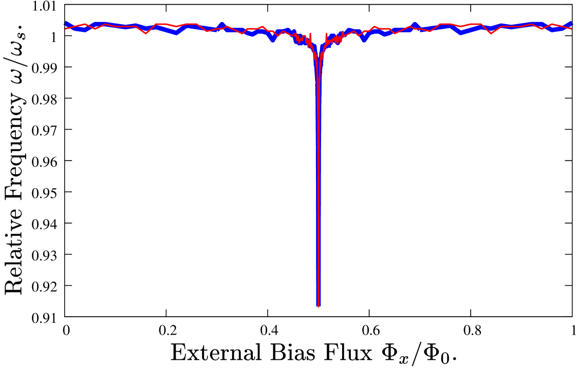
Figure 5: Frequency shift of a 130MHz tank circuit ($L_{tc}=3\times 10^{-8}H$, $C_{tc}=5\times 10^{-11}F$), coupled to the SQUID ring of figure 2, as a function of external applied flux for the ring in its ground state only (figure 2) calculated using the both the Born-Oppenheimer (in blue) and non-adiabatic (in red) approaches.

As our example of the frequency conversion process we consider a SQUID ring with circuit parameters used in the computed results of figures 2 and 4. For the SQUID ring parameters we have chosen the characteristic ring oscillator frequency to be close to $130\mathrm{GHz}$. Referring to the computed results of figure 4, we again choose the frequency for the microwave source to be $13\mathrm{GHz}$, i.e. an order of magnitude lower than the ring characteristic frequency, and set the tank circuit resonant frequency another two orders of magnitude lower (i.e. $130\mathrm{MHz}$). Within the limits of the computational power available to us this provides us with the opportunity to demonstrate extreme (1000:1), quantum SQUID ring mediated, energy down conversion.

With the results of figure 5 in support, and utilising the time averaged energy expectation results of figure 4 as a guide, we then proceeded to compute the energy transfer, via the SQUID ring, from input field to an undriven output tank circuit at selected flux bias points close to and within an exchange region in 4.

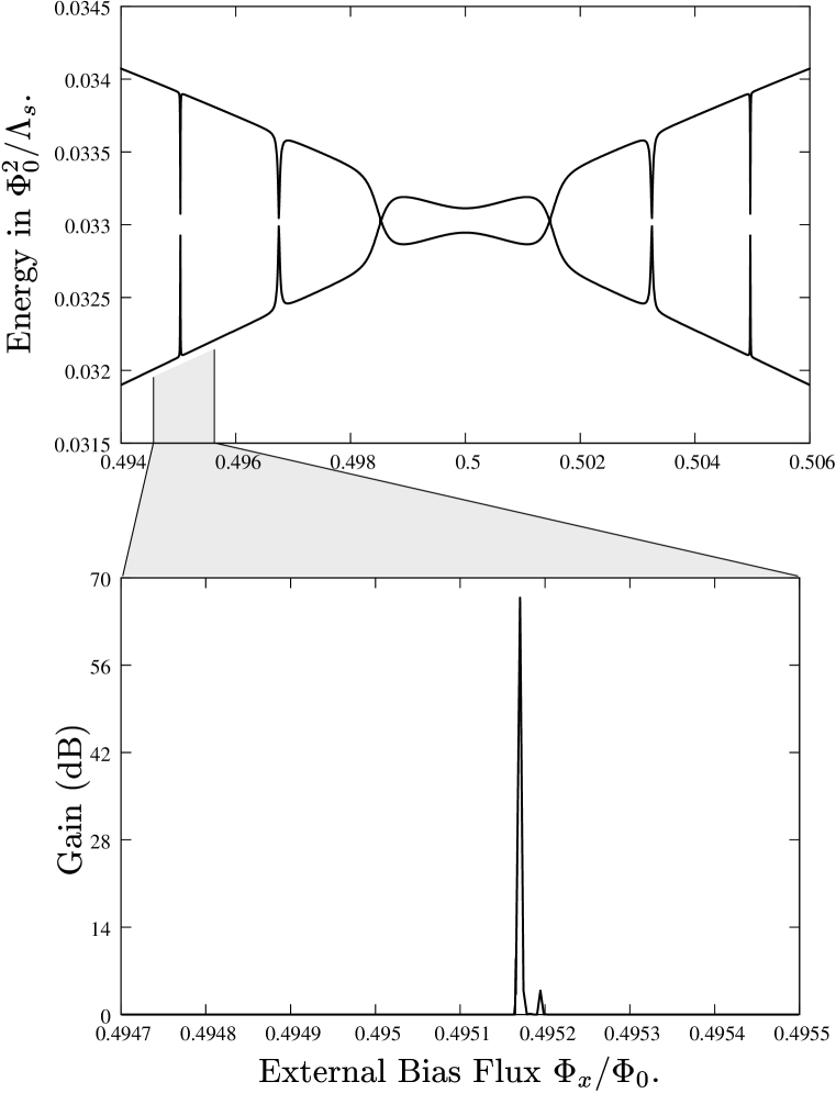
Figure 6: (top) reproduction of figure 4 illustrating the region of bias flux used to compute (bottom) the power gain in the tank circuit (with respect to $\Phi_{x}^{\mathrm{stat}}=0\Phi_{0}$). Here, the microwave source frequency was 13GHz which converted into the output (tank circuit) oscillator mode of 130MHz. As can be seen, the peak power at the centre of the exchange region is $\approx 70$dB above the background from outside the exchange region.

Our results are shown in figure 6 for the region of bias flux denoted using the time averaged energy expectation values at the top (which reproduces figure 4). As can be seen, outside the exchange region there is no evidence of energy conversion between the input microwave field and the output tank circuit. However, within the exchange region there is very significant conversion, reaching a maximum gain ($\approx 70$dB above background) at its centre.

The results we have presented in this paper demonstrate that a input-output frequency down conversion of a factor of a couple of orders of magnitude can be explained through the simple model we have utilised. However, this does not constitute a theoretical upper limit, only a practical constraint arising from the level of computational power available to us. We also note that by symmetry, and due to the fact that the SQUID ring couples different frequencies together, frequency up conversion via this same mechanism should also be possible.

V Conclusions

In this paper we have demonstrated that the interaction of a quantum mechanical SQUID ring with classical circuit environments is non-trivial. However, in the usual approach to the influence of a classical (and dissipative) circuit environment on the time evolution of a quantum mechanical SQUID ring r12 , it is assumed that the environment can be modelled by a bath of linear harmonic oscillators linearly coupled to the ring CL83 . This need not be the case. The highly non-perturbative nature of the SQUID ring in the quantum regime (and other Josephson weak link based circuits) means that the ring-environment interaction can be very non-linear and may lead to unexpected results. One of these is clearly the extreme frequency ratio conversion possible between classical fields via a quantum mechanical SQUID ring. Since the problem of environmental (dissipative, decohering) effects is so central to the successful implementation of quantum technologies, it is our opinion that for non-linear devices such as SQUID rings the role of the environment has to be reconsidered within this non-perturbative (non-linear) context.

On a purely experimental level the theoretical results generated in this paper indicate that quantum SQUID rings can be used for very large frequency ratio down conversion between classical fields. This seems to be supported by experiment r17 and may prove to be of considerable practical significance, especially with the current interest in classical THz communications technologies DLP04 .

VI Acknowledgements

We would like to thank the Engineering and Physical Sciences Research Council for supporting the work presented in this paper through its Quantum Circuits Network programme.

References

- (1) H. Lo, S. Popescu, and T.P. Spiller, Introduction to Quantum Computation and Information (World Scientific, New Jersey, 1998).
- (2) M.A. Nielsen, and I.L. Chuang, Quantum Computation and Quantum Information (Cambridge University Press, Cambridge, 2000).
- (3) The Physics of Quantum Information (eds. D. Bouwmeester, A. Ekert, and A. Zeilinger (Springer-Verlag, Berlin, 2000).
- (4) C.H. van der Wal, .C.J. ter Haar, F.K. Wilhelm, R.N. Schouten, C.J.P.M. Harmans, T.P. Orlando, S. Lloyd, and J.E. Mooij, Science 290, 773 (2000).
- (5) J.R. Friedman, V. Patel, W. Chen, S.K. Tolpygo, and J.E. Lukens, Nature (London) 406, 43 (2000).
- (6) Y.K. Nakamura, C.D. Chen, and J.S. Tsai, Phys. Rev. Lett. 79, 2328 (1997).
- (7) Y.K. Nakamura, Y.A. Pashkin, and J.S. Tsai, Nature (London), 398, 786 (1999).
- (8) J. Martinis, S. Nam, and J. Aumentado, Phys. Rev. Lett. 89, 117901 (2002).
- (9) P. Silvestrini, B.B. Ruggiero, C. Grananta and E. Esposito, Phys. Lett. A, 267, 45 (2000).
- (10) I. Chiorescu, Y. Nakamura, C. Harmans, and J.E. Mooij, Science 299, 1869 (2003).
- (11) T.P. Spiller, Fortschritte Der Physik - Progress in Physics - 48 (9-11): 1075 (2000).
- (12) U. Weiss, Quantum Dissipative systems (World Scientific, Singapore, 1999).
- (13) H.J. Carmichael, ”An Open Systems Approach to Quantum Optics”, (Lecture notes in physics M18), Springer, Berlin (1993).
- (14) A.J. Leggett, S. Chakravarty, A.T. Dorsey, M.P.A. Fisher, A. Garg, and W. Zwerger, Rev. Mod. Phys. 59, 1 (1987).
- (15) T.D. Clark, J.F. Ralph, R.J. Prance, H. Prance, J. Diggins, and R. Whiteman, Phys. Rev. E 57, 4035 (1998).
- (16) M.J. Everitt, P.B. Stiffell, T.D. Clark, A. Vourdas, J.F. Ralph, H. Prance, and R.J. Prance, Phys. Rev. B 63, 184517 (2001).
- (17) R. Whiteman, T.D. Clark, R.J. Prance, H. Prance, V. Schollmann, J.F. Ralph, M.J. Everitt and J. Diggins, J. Mod. Opt. 45:1175-1184, (1998).
- (18) W.T. Silfvast, ”Laser Fundamentals”, Cambridge University Press (1996).
- (19) J.F. Ralph, T.D. Clark, M.J. Everitt, H. Prance, P.B. Stiffell, and R.J. Prance, Phys. Lett. A 317, 199 (2003).
- (20) T.P. Orlando, J.E. Mooij, L. Tian, C.H. van der Wal, L.S. Levitov, S. Lloyd, and J.J. Mazo, Phys. Rev. B 60, 15398 (1999).
- (21) T.P. Spiller, T.D. Clark, R.J. Prance and A. Widom, Progress in Low Temperature Physics (Elsevier Science, Amserdam, 1992), Vol. XIII.
- (22) Y. Srivastava and A. Widom, Phys. Rep. 148, 1 (1987).
- (23) R. Whitemen, V. Schollmann, M.J. Everitt, T.D. Clark, R.J. Prance, H. Prance, J. Diggins, G. Buckling and J.F. Ralph, J. Phys.-Condes Matter, 10:9951-9968 (1998).
- (24) O.V. Lounasmaa, ”Experimental Principles and Methods below 1 K” (Academic Press, London, 1974), pp. 156-159.
- (25) K.K. Likharev, ”Dynamics of Josephson Junctions and Circuits” (Gordon and Breach, New York, 1986).
- (26) T.D. Clark, J. Diggins, J.F. Ralph, M.J. Everitt, R.J. Prance and H. Prance, R. Whiteman, A. Widom and Y.N. Srivastava, Ann. Phys. 268, 1 (1998).
- (27) M.J. Everitt, T.D. Clark, P.B. Stiffell, A. Vourdas, J.F. Ralph, R.J. Prance and H. Prance Phys. Rev A 69, 043804 (2004)
- (28) J.F. Ralph, T.D. Clark, M.J. Everitt, P.B. Stiffell, Phys. Rev. B 64, 180505 (2001).
- (29) A.O. Caldeira, A.J. Leggett, Ann. Phys. 149(2):374-456 (1983).
- (30) A.G. Davies, E.H. Linfield, M. Pepper, ”The terahertz gap: the generation of far-infrared radiation and its applications - Preface” Philos. T. Roy. Soc. A 362(1815):197-197 (2004).