Distribution of winners in truel games

Abstract

In this work we present a detailed analysis using the Markov chain theory of some versions of the truel game in which three players try to eliminate each other in a series of one-to-one competitions, using the rules of the game. Besides reproducing some known expressions for the winning probability of each player, including the equilibrium points, we give expressions for the actual distribution of winners in a truel competition.

1 Introduction

A truel is a game in which three players aim to eliminate each other in a series of one-to-one competitions. The mechanics of the game is as follows: at each time step, one of the players is chosen and he decides who will be his target. He then aims at this person and with a given probability he might achieve the goal of eliminating him from the game (this is usually expressed as the players “shooting” and “killing” each other, although possible applications of this simple game do not need to be so violent). Whatever the result, a new player is chosen amongst the survivors and the process repeats until only one of the three players remains. The paradox is that the player that has the highest probability of annihilating competitors does not need to be necessarily the winner of this game. This surprising result was already present in the early literature on truels, see the bibliography in the excellent review of reference KB97 . According to this reference, the first mention of truels was in the compendium of mathematical puzzles by Kinnaird kin46 although the name truel was coined by Shubik shu82 in the 1960s.

Different versions of the truels vary in the way the players are chosen (randomly, in fixed sequence, or simultaneous shooting), whether they are allowed to “pass”, i.e. missing the shoot on purpose (“shooting into the air”), the number of tries (or “bullets”) available for each player, etc. The strategy of each player consists in choosing the appropriate target when it is his turn to shoot. Rational players will use the strategy that maximizes their own probability of winning and hence they will chose the strategy given by the equilibrium Nash point. In a series of seminal papersk72.1 ; k75.1 ; k75.3 , Kilgour has analyzed the games and determined the equilibrium points under a variety of conditions.

In this paper, we analyze the games from the point of view of Markov chain theory. Besides being able to reproduce some of the results by Kilgour, we obtain the probability distribution for the winners of the games. We restrict our study to the case in which there is an infinite number of bullets and consider two different versions of the truel: random and fixed sequential choosing of the shooting player. These two cases are presented in sections 2 and 3, respectively. In section 4 we consider a variation of the game in which, instead of eliminating the competitors from the game, the objective is to convince them on a topic, making the truel suitable for a model of opinion formation. Some conclusions and directions for future work are presented in section 5 whereas some of the most technical parts of our work are left for the final appendixes.

2 Random firing

Let us first fix the notation. The three players are labeled as A,B,C. We denote by $a$, $b$ and $c$, respectively, their marksmanship, defined as the probability that a player has of eliminating from the game the player he has aimed at. The strategy of a player is the set of probabilities he uses in order to aim to a particular player or to shoot into the air. Obviously, when only two players remain, the only meaningful strategy is to shoot at the other player. If three players are still active, we denote by $P_{AB}$, $P_{AC}$ and $P_{A0}$ the probability of player A shooting into player B, C, or into the air, respectively, with equivalent definitions for players B and C. These probabilities verify $P_{AB}+P_{AC}+P_{C0}=1$. A “pure” strategy for player A corresponds to the case where one of these three probabilities is taken equal to 1 and the other two equal to 0, whereas a “mixed” strategy takes two or more of these probabilities strictly greater than 0. Finally, we denote by $\pi(a;b,c)$ the probability that the player with marksmanship $a$ wins the game when he plays against two players of marksmanship $b$ and $c$. The definition implies $\pi(a;b,c)=\pi(a;c,b)$ and $\pi(a;b,c)+\pi(b;a,c)+\pi(c;a,b)=1$.

In the particular case considered in this section, at each time step one of the players is chosen randomly with equal probability amongst the survivors. There are 7 possible states of this system labeled as ABC, AB, AC, BC, A, B, C, according to the players who remain in the game. The game can be thought of as a Markov chain with seven states, three of them being absorbent states. The details of the calculation for the winning probabilities of A, B and C as well as a diagram of the allowed transitions between states are left for the appendix 6.1. We now discuss the results in different cases.

Imagine that the players do not adopt any thought strategy and each one shoots randomly to any of the other two players. Clearly, this is equivalent to setting $P_{AB}=P_{AC}=P_{BA}=P_{BC}=P_{CA}=P_{CB}=1/2$. The winning probabilities in this case are:

$$\pi(a;b,c)=\frac{a}{a+b+c},~{}~{}~{}~{}\pi(b;a,c)=\frac{b}{a+b+c},~{}~{}~{}~{}\pi(c;a,b)=\frac{c}{a+b+c},$$ (1)

a logical result that indicates that the player with the higher marksmanship possesses the higher probability of winning. Identical result is obtained if the players include shooting in the air as one of their equally likely possibilities.

It is conceivable, though, that players will not decide the targets randomly, but will use some strategy in order to maximize their winning probability. Completely rational players will choose strategies that are best responses (i.e. strategies that are utility–maximizing) to the strategies used by the other players. This defines an equilibrium point when all the players are better off keeping their actual strategy than changing to another one. Accordingly, this equilibrium point can be defined as the set of probabilities $P_{\alpha\beta}$ (with $\alpha=$A,B,C and $\beta=$A,B,C,0) such that the winning probabilities have a maximum. This set can be found from the expressions in the appendix, with the result that the equilibrium point in the case $a>b>c$ is given by $P_{AB}=P_{CA}=P_{BA}=1$ and $P_{AC}=P_{A0}=P_{BC}=P_{B0}=P_{CB}=P_{C0}=0$. This is the “strongest opponent strategy” in which each player aims at the strongest of his opponentsKB97 . With this strategy, the winning probabilities are:

$$\pi(a;b,c)=\frac{a^{2}}{(a+c)(a+b+c)},~{}\pi(b;a,c)=\frac{b}{a+b+c},~{}\pi(c;a,b)=\frac{c(c+2a)}{(a+c)(a+b+c)}$$ (2)

(notice that these expressions assume $a>b>c$; other cases can be easily obtained by a convenient redefinition of $a$, $b$ and $c$).

An analysis of these probabilities leads to the paradoxical result that when all players use their ’best’ strategy, the player with the worst marksmanship can become the player with the highest winning probability. For example, if $a=1.0$, $b=0.8$, $c=0.5$ the probabilities of A, B and C winning the game are $0.290$, $0.348$ and $0.362$, respectively, precisely in inverse order of their marksmanship. The paradox is explained when one realizes that all players set as primary target either players $A$ or $B$, leaving player $C$ as the last option and so he might have the largest winning probability. In Fig.1 we plot the regions in parameter space $(b,c)$ (after setting $a=1$) representing the player with the highest winning probability.

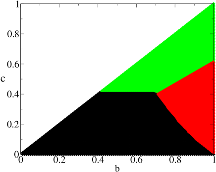
Figure 1: In the parameter space $(b,c)$ with $c<b<a=1$, we indicate by black (resp. dark gray, light gray) the regions in which player A (resp. B, C) has the largest probability of winning the truel in the case of random selection of the shooting player and the use of the optimal strategy, as given by Eq. (2).

Imagine that we set up a truel competition. Sets of three players are chosen randomly amongst a population whose marksmanship are uniformly distributed in the interval $(0,1)$. The distribution of winners is characterized by a probability density function, $f(x)$, such that $f(x)dx$ is the proportion of winners whose marksmanship lies in the interval $(x,x+dx)$. This distribution is obtained as:

$$f(x)=\int da\,db\,dc\,\left[\pi(a;b,c)\delta(x-a)+\pi(b;a,c)\delta(x-b)+\pi(c;a,b)\delta(x-c)\right]$$ (3)

or

$$f(x)=3\int_{0}^{1}db\int_{0}^{1}dc\,\pi(x;b,c)$$ (4)

If players use the random strategy, Eq. (1), the distribution of winners is $f(x)=3x\left[x\ln x-2(1+x)\ln(1+x)+(2+x)\ln(2+x)\right]$. In figure 2 we observe that, as expected, the function $f(x)$ attains its maximum at $x=1$ indicating that the best marksmanship players are the ones which win in more occasions.

We consider now a variation of the competition in which the winner of one game keeps on playing against other two randomly chosen players. The resulting distribution of players, $\bar{f}(x)$, can be computed as the steady state solution of the recursion equation:

$$\bar{f}(x,t+1)=\int da\,db\,dc\,\left[\pi(a;b,c)\delta(x-a)+\pi(b;a,c)\delta(x-b)+\pi(c;a,b)\delta(x-c)\right]\bar{f}(a,t)$$ (5)

or

$$\bar{f}(x)=\frac{1}{3}\bar{f}(x)f(x)+2\int_{0}^{1}db\int_{0}^{1}dc\,\pi(x;b,c)\bar{f}(b)$$ (6)

In the case of using the probabilities of Eq. (1) the distribution of winners is $\bar{f}(x)=2x$.

For players adopting the equilibrium point strategy, Eq.(2), the resulting expression for $f(x)$ is too ugly to be reproduced here, but the result has been plotted in Fig. 3. Notice that, despite the paradoxical result mentioned before, the distribution of winners still has it maximum at $x=1$, indicating that the best marksmanship players are nevertheless the ones who win in more occasions. In the same figure, we have also plotted the distribution $\bar{f}(x)$ of the competition in which the winner of a game keeps on playing. In this case, the integral relation Eq.(6) has been solved numerically.

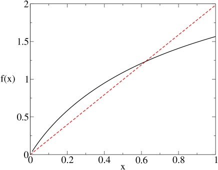
Figure 2: Distribution function $f(x)$ for the winners of truels of randomly chosen triplets (solid line) in the case of players using random strategies, Eq. (1); distribution $\bar{f}(x)$ of winners in the case where the winner of a truel remains in the competition (dashed line).

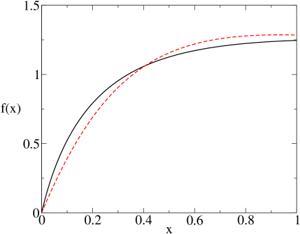
Figure 3: Similar to Fig.(2) in the case of the competition where players use the rational strategy of the equilibrium point given by eq.(2).

3 Sequential firing

In this version of the truel there is an established order of firing. The players will shoot in increasing value of their marksmanship. i.e. if $a>b>c$ the first player to shoot will be player $C$, followed by player $B$ and the last to shoot is player $A$. The sequence repeats until only one player remains. Again, we have left for the appendix 6.2 the details of the calculation of the winning probabilities. Our analysis of the optimal strategies reproduces that obtained by the detailed study of Kilgourk75.1 . The result is that there are two equilibrium points depending on the value of the function $g(a,b,c)=a^{2}(1-b)^{2}(1-c)-b^{2}c-a\,b\,(1-b\,c)$: if $g(a,b,c)>0$ the equilibrium point is the strongest opponent strategy $P_{AB}=P_{BA}=P_{CA}=1$, while for $g(a,b,c)<0$ it turns out that the equilibrium point strategy is $P_{AB}=P_{BA}=P_{C0}=1$ where the worst player C is better off by shooting into the air and hoping that the second best player B succeeds in eliminating the best player A from the game.

The winning probabilities for this case, assuming $a>b>c$, are:

$$\pi(a;b,c) = \frac{(1-c)(1-b)a^{2}}{[c(1-a)+a][b(1-a)+a]},$$

$$\pi(b;a,c) = \frac{(1-c)b^{2}}{(c(1-b)+b)(b(1-a)+a)},$$

$$\pi(c;a,b) = \frac{c[bc+a[b(2+b(-1+c)-3c)+c]]}{[c+a(1-c)][b+a(1-b)][a+b(1-a)]},$$ (7)

if $g(a,b,c)>0$, and

$$\pi(a;b,c) = \frac{a^{2}(1-b)(1-c)^{2}}{[a+(1-a)c][a+b(1-a)+c(1-a)(1-b)]},$$

$$\pi(b;a,c) = \frac{b\left(b(1-c)^{2}+c\right)}{[b+(1-b)c][a+b(1-a)+c(1-a)(1-b)]},$$

$$\pi(c;a,b) = \frac{\frac{ac(1-b)(1-c)}{a+c(1-a)}+\frac{c(b+c(1-2b))}{b+c(1-b)}}{[a+b(1-a)+c(1-a)(1-b)]},$$ (8)

if $g(a,b,c)<0$. Again, as in the case of random firing, the paradoxical result appears that the player with the smallest marksmanship has the largest probability to win the game. In figure 4 we summarize the results indicating the regions in parameter space $(b,c)$ (with $a=1$) where each player has the highest probability of winning. Notice that the ’best’ player A has a much smaller region of winning than compared with the case of random firing.

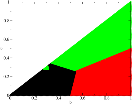
Figure 4: Same as Fig.1 in the case that players play sequentially in increasing order of their marksmanship.

In figure 5 we plot the distribution of winners $f(x)$ and $\bar{f}(x)$ in a competition as defined in the previous section. Notice that now the distribution of winners $f(x)$ has a maximum at $x\approx 0.57$ indicating that the players with the best marksmanship do not win in the majority of cases.

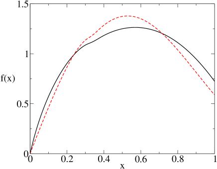
Figure 5: Same as Fig.2 in the case that players play sequentially in increasing order of their marksmanship. Notice that now both distributions of winners present maxima for $x<1$ indicating that the best a priori players do not win the game in the majority of the cases.

4 Convincing opinion

We reinterpret the truel as a game in which three people holding different opinions, A, B and C, on a topic, aim to convince each other in a series of one-to-one discussions. The marksmanship $a$ (resp. $b$, $c$) are now interpreted as the probabilities that player holding opinion A (resp. B or C) have of convincing another player of adopting this opinion. The main difference with the previous sections is that now there are always three players present in the game and the different states in the Markov chain are ABC, AAB, ABB, AAC, ACC, BBC, BCC, AAA, BBB and CCC. The analysis of the transition probabilities is left for appendix 6.3. We consider only the random case in which the person that tries to convince another one is chosen randomly amongst the three players. The equilibrium point corresponds to the best opponent strategy set of probabilities in which each player tries to convince the opponent with the highest marksmanship. The probabilities that the final consensus opinion is A, B or C, assuming $a>b>c$ are given by

$$\pi(a;b,c) = \frac{a^{2}\left[2cb^{2}+a\left((a+b)^{2}+2(a+2b)c\right)\right]}{(a+b)^{2}(a+c)^{2}(a+b+c)},$$

$$\pi(b;a,c) = \frac{b^{2}(b+3c)}{(b+c)^{2}(1+b+c)},$$

$$\pi(c;a,b) = \frac{c^{2}\left[c^{3}+3(a+b)c^{2}+a(a+8b)c+ab(3a+b)\right]}{(a+c)^{2}(b+c)^{2}(a+b+c)},$$ (9)

respectively. As shown in Fig. 6, there is still a set of parameter values $(a,b,c)$ for which opinion C has the highest winning probability, although it is smaller than in the versions considered in the previous sections.

Similarly to other versions, we plot in figure 7 the distribution of winning opinions, $f(x)$. Notice that, as in the random firing case, it attains its maximum at $x=1$ showing that the most convincing players win the game in more occasions. We have also plotted in the same figure, the distribution $\bar{f}(x)$ which results where one of the winners of a truel is kept to discuss with two randomly chosen players in the next round.

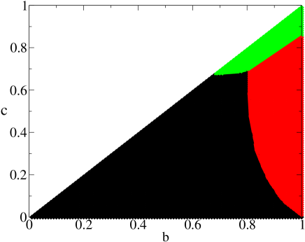
Figure 6: Same as Fig.1 for the convincing opinion model.

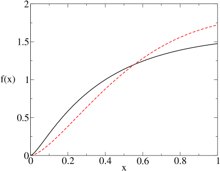
Figure 7: Same as Fig.2 for the convincing opinion model.

5 Conclusions

As discussed in the review of reference KB97 , truels are of its interest in many areas of social and biological sciences. In this work, we have presented a detailed analysis of the truels using the methods of Markov chain theory. We are able to reproduce in a language which is more familiar to the Physics community most of the results of the alternative analysis by Kilgourk75.1 . Besides computing the optimal rational strategy, we have focused on computing the distribution of winners in a truel competition. We have shown that in the random case, the distribution of winners still has its maximum at the highest possible marksmanship, $x=1$, despite the fact that sometimes players with a lower marksmanship have a higher probability of winning the game. In the sequential firing case, the paradox is more present since even the distribution of winners has a maximum at $x<1$. It would be interesting to determine mechanisms by which players could, in an evolutionary scheme, adapt themselves to the optimal values.

6 Appendix: Calculation of the probabilities

6.1 Random firing

In this game there are seven possible states according to the remaining players. These are labeled as $0,1,\dots,6$. There are transitions between those states, as shown in the diagram in Fig. 8, where $p_{ij}$ denotes the transition probability from state $i$ to state $j$ (the self–transition probability $p_{ii}$ is denoted by $r_{i}$).

States	Remaining players
$0$	ABC
$1$	AB
$2$	AC
$3$	BC
$4$	A
$5$	B
$6$	C

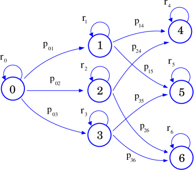
Figure 8: Table with the description of all the possible states for the random firing game, and diagram representing the allowed transitions between the states shown in the table.

From Markov chain theoryk75.2 we can evaluate the probability $u^{j}_{i}$ that starting from state $i$ we eventually end up in state $j$ after a sufficiently large number of steps. In particular, if we start from state $0$ (with the three players active), the nature of the game is such that the only non-vanishing probabilities are $u_{0}^{4}$, $u_{0}^{5}$ and $u_{0}^{6}$ corresponding to the winning of the game by player A, B and C respectively. The relevant set of equations is :

$$\begin{array}[]{lll}&u_{0}^{4}=p_{01}~{}u_{1}^{4}+p_{02}~{}u_{2}^{4}+p_{03}~{}u_{3}^{4}+r_{0}~{}u_{0}^{4},&u_{0}^{5}=p_{01}~{}u_{1}^{5}+p_{02}~{}u_{2}^{5}+p_{03}~{}u_{3}^{5}+r_{0}~{}u_{0}^{5},\\ &u_{1}^{4}=p_{14}~{}u_{4}^{4}+r_{1}~{}u_{1}^{4},&u_{1}^{5}=p_{15}~{}u_{5}^{5}+r_{1}~{}u_{1}^{5},\\ &u_{2}^{4}=p_{24}~{}u_{4}^{4}+r_{2}~{}u_{2}^{4},&u_{2}^{5}=r_{2}~{}u_{2}^{5},\\ &u_{3}^{4}=r_{3}~{}u_{3}^{4},&u_{3}^{5}=r_{3}~{}u_{3}^{5}+p_{35}~{}u_{5}^{5}.\end{array}$$

Solving for $u_{0}^{4}$, $u_{0}^{5}$ and $u_{0}^{6}$ we obtain:

$$u_{0}^{4} =\frac{p_{01}~{}p_{14}}{(1-r_{0})(1-r_{1})}+\frac{p_{02}~{}p_{24}}{(1-r_{0})(1-r_{2})},$$

$$u_{0}^{5} =\frac{p_{01}~{}p_{15}}{(1-r_{0})(1-r_{1})}+\frac{p_{03}~{}p_{35}}{(1-r_{0})(1-r_{3})},$$

$$u_{0}^{6} =\frac{p_{02}~{}p_{26}}{(1-r_{0})(1-r_{2})}+\frac{p_{03}~{}p_{36}}{(1-r_{0})(1-r_{3})}.$$

We can now derive the expressions for the transition probabilities $p_{ij}$. Remember that we denote by $a$ the probability that player A eliminates from the game the player he has aimed at (and similarly for $b$ and $c$), and that $P_{\alpha\beta}$ ($\alpha=$A,C,B and $\beta=$ A,B,C,0) the probability of player $\alpha$ choosing player $\beta$ (or into the air if $\beta=0$) as a target when it is his turn to play (a situation that only appears when the three players are still active). We have then:

$$\begin{array}[]{lll}&r_{0}=1-\frac{1}{3}(a(1-P_{A0})+b(1-P_{B0})+c(1-P_{C0})),&p_{01}=\frac{1}{3}(aP_{AC}+bP_{BC}),\\ &p_{02}=\frac{1}{3}(aP_{AB}+cP_{CB}),&p_{03}=\frac{1}{3}(bP_{BA}+cP_{CA}),\\ &p_{14}=p_{24}=\frac{1}{2}a,&p_{15}=p_{35}=\frac{1}{2}b,\\ &p_{26}=p_{36}=\frac{1}{2}c,&r_{1}=1-\frac{1}{2}(a+b),\\ &r_{2}=1-\frac{1}{2}(a+c),&r_{3}=1-\frac{1}{2}(b+c).\end{array}$$ (11)

6.2 Sequential firing

As in the random firing case, we describe this game as a Markov chain composed of $11$ different states, also with three absorbent states: $9$ , $10$ and $11$. In Fig. 9 we can see the corresponding diagram for this game, together with a table describing all possible states. Based on this diagram, we can write down the relevant set of equations for the transition probabilities $u_{i}^{j}$:

States	Remaining players
$0$	A B C
$1$	A B C
$2$	A B C
$3$	B C
$4$	A C
$5$	B C
$6$	A B
$7$	A C
$8$	A B
$9$	C
$10$	B
$11$	A

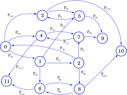
Figure 9: Table: Description of the different states of the game for the case of sequential firing. The highlighted player is the one chosen for shooting in that state. Diagram: scheme representing all the allowed transitions between the states shown in the table for the case of a truel with sequential firing in the order C$\to$ B $\to$ A with $a>b>c$.

$$\begin{array}[]{llll}\vspace{0.2cm}&u_{0}^{9}=p_{03}u_{3}^{9}+p_{01}u_{1}^{9}+p_{04}u_{4}^{9},&u_{0}^{10}=p_{03}u_{3}^{10}+p_{01}u_{1}^{10},&u_{0}^{11}=p_{01}u_{1}^{11}+p_{04}u_{4}^{11},\\ \vspace{0.2cm}&u_{1}^{10}=p_{12}u_{2}^{10}+p_{15}u_{5}^{10}+p_{16}u_{6}^{10},&u_{1}^{9}=p_{12}u_{2}^{9}+p_{15}u_{5}^{9},&u_{1}^{11}=p_{12}u_{2}^{11}+p_{16}u_{6}^{11},\\ \vspace{0.2cm}&u_{2}^{11}=p_{28}u_{8}^{11}+p_{27}u_{7}^{11}+p_{20}u_{0}^{11},&u_{2}^{9}=p_{27}u_{7}^{9}+p_{20}u_{0}^{9},&u_{2}^{10}=p_{28}u_{8}^{10}+p_{20}u_{0}^{10},\\ \vspace{0.2cm}&u_{3}^{9}=p_{35}u_{5}^{9},&u_{3}^{10}=p_{35}u_{5}^{10}+p_{3\,10},\\ \vspace{0.2cm}&u_{4}^{9}=p_{47}u_{7}^{9},&u_{4}^{11}=p_{47}u_{7}^{11}+p_{4\,11},\\ \vspace{0.2cm}&u_{5}^{9}=p_{53}u_{3}^{9}+p_{59},&u_{5}^{10}=p_{53}u_{3}^{10},\\ \vspace{0.2cm}&u_{6}^{10}=p_{68}u_{8}^{10},&u_{6}^{11}=p_{68}u_{8}^{11}+p_{6\,11},\\ \vspace{0.2cm}&u_{7}^{9}=p_{74}u_{4}^{9}+p_{79},&u_{7}^{11}=p_{74}u_{4}^{11},\\ \vspace{0.2cm}&u_{8}^{10}=p_{86}u_{6}^{10}+p_{8\,10},&u_{8}^{11}=p_{86}u_{6}^{11}.\end{array}$$ (12)

The general solutions for the probabilities $u_{0}^{9}$, $u_{0}^{10}$ and $u_{0}^{11}$ are given by

$$u_{0}^{9} = \frac{1}{1-p_{01}p_{12}p_{20}}\left[\frac{p_{59}(p_{03}p_{35}+p_{01}p_{15})}{1-p_{35}p_{53}}+\frac{p_{79}(p_{04}p_{47}+p_{01}p_{12}p_{27})}{1-p_{47}p_{74}}\right],$$

$$u_{0}^{10} = \frac{1}{1-p_{01}p_{12}p_{20}}\left[\frac{p_{3\,10}(p_{03}+p_{01}p_{15}p_{53})}{1-p_{35}p_{53}}+\frac{p_{01}p_{8\,10}(p_{16}p_{68}+p_{12}p_{28})}{1-p_{68}p_{86}}\right],$$ (13)

$$u_{0}^{11} = \frac{1}{1-p_{01}p_{12}p_{20}}\left[\frac{p_{4\,11}(p_{04}+p_{01}p_{12}p_{27}p_{74})}{1-p_{47}p_{74}}+\frac{p_{01}p_{6\,11}(p_{16}+p_{12}p_{28}p_{86})}{1-p_{68}p_{86}}\right],$$

with transition probabilities given by

$$\begin{array}[]{llll}&p_{01}=(1-c)+cP_{C0},&p_{03}=cP_{CA},&p_{04}=cP_{CB},\\ &p_{12}=(1-b)+bP_{B0},&p_{15}=bP_{BA},&p_{16}=bP_{CA},\\ &p_{20}=(1-a)+aP_{A0},&p_{27}=aP_{AB},&p_{28}=aP_{AC},\\ &p_{35}=p_{86}=1-b,&p_{3\,10}=p_{8\,10}=b,\\ &p_{47}=p_{68}=1-a,&p_{4\,11}=p_{6\,11}=a,\\ &p_{53}=p_{74}=1-c,&p_{59}=p_{79}=c.\end{array}$$

6.3 Convincing opinion

For this model we show in Fig. 10 the diagram of all the allowed states and transitions, together with a table describing the possible states.

States	Opinions
$0$	A B C
$1$	A A A
$2$	B B B
$3$	C C C
$4$	A A B
$5$	A B B
$6$	A A C
$7$	A C C
$8$	B B C
$9$	B C C

Figure 10: Table: description of the different states of the opinion model. Diagram: scheme representing the allowed transitions between the states.

The corresponding set of equations describing this convincing opinion model, as derived from the diagram, are

$$\begin{array}[]{lll}&u_{0}^{1}=r_{0}u_{0}^{1}+p_{06}u_{6}^{1}+p_{04}u_{4}^{1}+p_{05}u_{5}^{1}+p_{07}u_{7}^{1},\\ &u_{0}^{2}=r_{0}u_{0}^{2}+p_{04}u_{4}^{2}+p_{05}u_{5}^{2}+p_{08}u_{8}^{2}+p_{09}u_{9}^{2},\\ &u_{0}^{3}=r_{0}u_{0}^{3}+p_{08}u_{8}^{3}+p_{09}u_{9}^{3}+p_{07}u_{7}^{3}+p_{06}u_{6}^{3},\\ &u_{4}^{1}=r_{4}u_{4}^{1}+p_{45}u_{5}^{1}+p_{41},&u_{4}^{2}=r_{4}u_{4}^{2}+p_{45}u_{5}^{2},\\ &u_{5}^{1}=r_{5}u_{5}^{1}+p_{54}u_{4}^{1},&u_{5}^{2}=r_{5}u_{5}^{2}+p_{54}u_{4}^{2}+p_{52},\\ &u_{6}^{1}=r_{6}u_{6}^{1}+p_{67}u_{7}^{1}+p_{61},&u_{6}^{3}=r_{6}u_{6}^{3}+p_{67}u_{7}^{3},\\ &u_{7}^{1}=r_{7}u_{7}^{1}+p_{76}u_{6}^{1},&u_{7}^{3}=r_{7}u_{7}^{3}+p_{76}u_{6}^{3}+p_{73},\\ &u_{8}^{2}=r_{8}u_{8}^{2}+p_{89}u_{9}^{2}+p_{82},&u_{8}^{3}=r_{8}u_{8}^{3}+p_{89}u_{9}^{3},\\ &u_{9}^{2}=r_{9}u_{9}^{2}+p_{98}u_{8}^{2},&u_{9}^{3}=r_{9}u_{9}^{3}+p_{98}u_{8}^{3}+p_{93}.\end{array}$$ (14)

And the general solution for the probabilities $u_{0}^{1}$, $u_{0}^{2}$ and $u_{0}^{3}$ is

$$u_{0}^{1} = \frac{1}{1-r_{0}}\left[\frac{p_{61}(p_{06}(1-r_{7})+p_{07}p_{76})}{(1-r_{6})(1-r_{7})-p_{67}p_{76}}+\frac{p_{41}(p_{04}(1-r_{5})+p_{05}p_{54})}{(1-r_{4})(1-r_{5})-p_{45}p_{54}}\right],$$

$$u_{0}^{2} = \frac{1}{1-r_{0}}\left[\frac{p_{52}(p_{04}p_{45}+p_{05}(1-r_{4}))}{(1-r_{4})(1-r_{5})-p_{45}p_{54}}+\frac{p_{82}(p_{08}(1-r_{9})+p_{09}p_{98})}{(1-r_{8})(1-r_{9})-p_{89}p_{98}}\right],$$

$$u_{0}^{3} = \frac{1}{1-r_{0}}\left[\frac{p_{73}(p_{06}p_{67}+p_{07}(1-r_{6}))}{(1-r_{6})(1-r_{7})-p_{67}p_{76}}+\frac{p_{93}(p_{09}(1-r_{8})+p_{08}p_{89})}{(1-r_{8})(1-r_{9})-p_{89}p_{98}}\right],$$ (15)

where the transition probabilities are given by

$$\begin{array}[]{llll}&p_{04}=\frac{1}{3}cP_{CA},&p_{06}=\frac{1}{3}cP_{CB},&p_{08}=\frac{1}{3}bP_{BC},\\ &p_{05}=\frac{1}{3}bP_{BA},&p_{07}=\frac{1}{3}aP_{AB},&p_{09}=\frac{1}{3}aP_{AC},\\ &p_{41}=p_{61}=\frac{2}{3}c&p_{45}=p_{98}=\frac{1}{3}b,&p_{54}=p_{76}=\frac{1}{3}c,\\ &p_{52}=p_{82}=\frac{2}{3}b,&p_{67}=p_{89}=\frac{1}{3}a,&p_{73}=p_{93}=\frac{2}{3}a,\\ &r_{0}=\frac{1}{3}[3-a-b-c],&r_{4}=\frac{2}{3}(1-c)+\frac{1}{3}(1-b),&r_{5}=\frac{1}{3}(1-c)+\frac{2}{3}(1-b),\\ &r_{6}=\frac{2}{3}(1-c)+\frac{1}{3}(1-a),&r_{7}=\frac{1}{3}(1-c)+\frac{2}{3}(1-a),&r_{8}=\frac{2}{3}(1-b)+\frac{1}{3}(1-a),\\ &r_{9}=\frac{1}{3}(1-b)+\frac{2}{3}(1-a).&&\end{array}$$ (16)

References

- (1) D.M. Kilgour and and S.J. Brams, The truel. Mathematics Magazine 1997, 70, 315.
- (2) C. Kinnaird, Encyclopedia of Puzzles and Pastimes, 1946, Citadel, Secaucus, NJ (USA).
- (3) M. Shubik, Game Theory in the Social Sciences 1982, MIT Press, Cambridge, MA (USA).
- (4) Kilgour, D. M., The simultaneous truel. Int. Journal of Game Theory, 1972, 1, 229–242.
- (5) Kilgour, D. M., The sequential truel. Int. Journal of Game Theory, 1975, 4, 151–174.
- (6) Kilgour, D. M., Equilibrium points of infinite sequential truels. Int. Journal of Game Theory, 1977, 6, 167–180.
- (7) Karlin, S., A first course in stochastic processes. Academic Press, New York, 1973.