Renormalization Group calculations with $k_{\|}$ dependent couplings in a ladder

Abstract

We calculate the phase diagram of a ladder system, with a Hubbard interaction and an interchain coupling $t_{\perp}$. We use a Renormalization Group method, in a one loop expansion, introducing an original method to include $k_{\|}$ dependence of couplings. We also classify the order parameters corresponding to ladder instabilities. We obtain different results, depending on whether we include $k_{\|}$ dependence or not. When we do so, we observe a region with large antiferromagnetic fluctuations, in the vicinity of small $t_{\perp}$, followed by a superconducting region with a simultaneous divergence of the Spin Density Waves channel. We also investigate the effect of a non local backward interchain scattering : we observe, on one hand, the suppression of singlet superconductivity and of Spin Density Waves, and, on the other hand, the increase of Charge Density Waves and, for some values of $t_{\perp}$, of triplet superconductivity. Our results eventually show that $k_{\|}$ is an influential variable in the Renormalization Group flow, for this kind of systems.

1 Introduction

The physics of ladder systems remains a source of considerable interest. In the last decades, many conductors were found, with anisotropic two-leg electronic structure, such as $SrCu_{2}O_{3}$[1] or $Sr_{14-x}Ca_{x}Cu_{24}O_{41}$[2] compounds. The structure of $La_{2}Cu_{2}O_{5}$[3] can also be analyzed as weakly coupled ladders, and is therefore very similar. The phase diagram of these compounds is very rich; it is now well established that these systems behave like Luttinger liquids at high temperature, while they can behave like Fermi liquids when $T$ decreases; they exhibit superconducting (SC) phases of type II, which can also be mixed with antiferromagnetic fluctuations. In some case, the SC phase is found to be spin-gapped, while spinless phases are also reported[4].

From a theoretical point of view, the ladder (or two-coupled chain) model is the simplest quasi-one-dimensional one. Although all its properties are not entirely elucidated, it has been used by many authors as a toy-model, to build and explore new approaches (two-leaf dispersion models calculated by a Kadanoff-Wilson renormalization method[5] or by a bosonization method[6]; transition between commensurate and incommensurate filling[7], in particular close to the half-filing case[8, 9]; dimensional transition[10], etc.). These systems have been intensively used to investigate non conventional SC process (with singlet[11, 12, 13] or triplet[14] pairing).

This paper is devoted to the study of a ladder model, with a Hubbard interaction ($U$ is the Hubbard constant) and an interband coupling ($t_{\perp}$ is the interaction factor), at zero temperature. We investigate the phase diagram in the range of parameter $0\leq U\leq 8\pi t_{\|}\eta$ and suppose that the electronic filling $\eta$ is incommensurate. Although there is yet no evidence for the existence of compounds lying in this range of parameter, we have hopes that some of these will indeed be found and confirm the theoretical predictions that we present here.

The phase diagram of this system has been partially studied by several authors. In particular, M. Fabrizio have used a Renormalization Group (RG) method, in a two-loop expansion from the Fermi liquid solution[12]. He includes interband backward scattering $g_{b}$, and, within the range of parameter that we have investigated, finds a SC phase, named ‘phase I’, which he clearly points out not to be singlet $s$, although he did not elucidate the symmetry of the condensate. In his calculations, the RG flow of susceptibilities shows several divergences : the Spin Density Wave (SDW) channel coexists with the superconducting one. This author did alternatively cut the flow before the divergences and bozonize the effective Hamiltonian; then, SDW modes disappear and are replaced by Charge Density Wave (CDW) instabilities.

These results are more or less compatible with that of other methods, using a one-loop expansion[15, 16], or bozonizing the Hamiltonian of the bare system[17, 18, 19, 20] (see also Ref. [13]), or using Quantum Monte Carlo method[21]. These authors generally find a singlet superconducting condensate of symmetry $d$, which coexists with SDW or CDW instabilities. This complicated phase has also been related to the RVB phase[22]. One of the central question is whether the SC modes are spin-gapped or not, and receives various and even contradictory answers. Using a two-loop expansion, Kishine[23] observes a spin gap, which is suppressed when $t_{\perp}\to 0$. This is also the result found with a Density Matrix RG method by Park[24].

We give a new insight into these questions, using a RG method, in a perturbative expansion in $U$. This kind of method has been used in many recent and very complete works[25, 26, 27]. Here, we calculate RG equations with one loop diagrams, including $g_{b}$ couplings, as in Ref. [12], as well as all parallel momentum dependence.

Let us emphasize that, although we begin from the Fermi liquid solution, we find a phase with only SDW fluctuations, for small enough interband interaction $t_{\perp}\leq t_{\perp c}(U)$, contrary to all previous results obtained by RG

methods, which always indicate SC instabilities as soon as $t_{\perp}\neq 0$ (see for instance Lin et al.[15]). However, this phase is different from the one-dimension limit. This is a very remarkable result, since $k_{\|}$ is known to be an irrelevant variable of the RG flow[28]. However, we will prove in this paper that it is indeed influential in the very case of a ladder.

When $t_{\perp}$ is increased, we observe a transition at $t_{\perp c}$ to a superconducting phase, where singlet SC instabilities of symmetry $d$ coexist with SDW ones. This phase is found by many authors (see Refs. [12, 15, 16] and other articles already quoted).

Recently, Bourbonnais et al.[29, 30] have examined the effect of interchain Coulomb interactions for an infinite number of coupled chains, using RG method. Interchain backward scattering was found to enhance CDW fluctuations and favor triplet instead of singlet SC. We here investigated the effect of a Coulomb interchain backward interaction $C_{\rm back}$ for the ladder problem. We find that this interaction favors triplet SC instabilities instead of singlet ones and CDW instabilities instead of SDW ones in a ladder system too. Indeed, both the singlet SC and SDW instabilities (if any) are suppressed when $C_{\rm back}$ is increased, and we observe triplet SC as well as CDW instabilities. The triplet SC existence region is however very narrow and lies inside the region $t_{\perp}\geq t_{\perp c}(U)$. For large values of $C_{\rm back}$ ($C_{\rm back}\sim U$), CDW is always dominant; this is consistent with what Lin et al. find[15].

On the contrary, when a Coulombian interchain forward interaction $C_{\rm for}$ is added, all SC instabilities are depressed, and we only observe SDW and CDW fluctuations.

We also present a detailed classification of the pair operators in a ladder, which are connected to the order parameters. It proves a very powerful tool in these sophisticated RG methods.

So, we will first give a short description of the model (in section 2), then present the classification of the pair operators (in section 3, the symmetries are explained in appendix C), then we explain the RG formulation and techniques that are used here (in section 4). Results concerning only initially local interactions are presented in section 5, while those concerning the influence of additional interchain interactions are given in section 6. In section 7 we conclude.

2 Model

The Hubbard model of a ladder has been studied in various articles. We give here a brief presentation of this model (see Refs. [12] or [31] with similar notations).

a Kinetic Hamiltonian

a.1 The model in a 1-$d$ representation

The dispersion curve separates into two bands (0 and $\pi$), so the Fermi surface splits into four points ($-k_{f0}$, $-k_{f\pi}$, $k_{f\pi}$, $k_{f0}$ in the $\|$ direction, + corresponds to right moving particles and $-$ to left moving ones). The bands are linearized around the Fermi vectors[32] with a single Fermi velocity $v_{f}$ (cf. Fig. 1). We write $R$ the right moving particles and $L$ the left moving ones. Then, the kinetic Hamiltonian writes

$$H_{\rm cin} = \sum_{\sigma}v_{f}\Big{(}\sum_{K}(K-k_{f0})R^{\dagger}_{0\sigma}(K)R_{0\sigma}(K)+\sum_{K}(K-k_{f\pi})R^{\dagger}_{\pi\sigma}(K)R_{\pi\sigma}(K)$$ (1)

$$+\sum_{K}(K+k_{f0})L^{\dagger}_{0\sigma}(K)L_{0\sigma}(K)+\sum_{K}(K+k_{f\pi})L^{\dagger}_{\pi\sigma}(K)L_{\pi\sigma}(K)\Big{)}.$$

We define the Fermi surface gap $\Delta k_{f}=k_{f0}-k_{f\pi}$. One then gets $\Delta k_{f}=2t_{\perp}/v_{f}$. The discretization step in $\|$ direction is $a$, and the reciprocal vector in this direction is defined modulo $2\pi/a$. The distance between the chains in $\perp$ direction is $b$.

Figure 1: The 2-band dispersion in $\|$ direction

In order to give a clear representation of all instability processes that will be discussed afterwards, it is worth showing how this model can be embedded in a 2-$d$ representation, which we present now.

a.2 The model in a 2-$d$ representation

The general 2-$d$ dispersion law writes

$$\epsilon({\bf k})=-2t_{\|}\cos(k_{\|}a)-2t_{\perp}\cos(k_{\perp}b)$$

as represented in Fig. 2; if one writes approximately $k_{f}\approx k_{f0}\approx k_{f\pi}$, one gets $v_{f}\approx 2at_{\|}\sin(k_{f}a)$. In real space, $y_{\|}$ corresponds to the axis along the chains, and $y_{\perp}$ takes only two values, $y_{\perp}=\pm 1$, corresponding to which chain one refers to. The $\|$ axis is then discretized, $y_{\|}=1\cdot\cdot N$, where $4N$ is the total number of states. The Fourier transformation from real space functions to reciprocal space ones is detailed in appendix D.

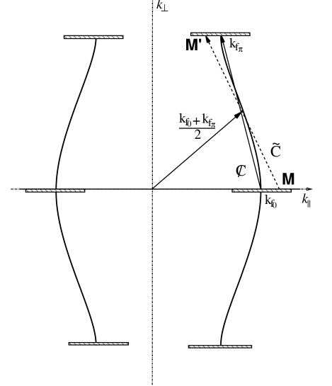
Figure 2: Two-dimensional representation of the states. The physical space, for a ladder, is restricted to the hatched bands at $k_{\perp}=0$ and $k_{\perp}=\pm{\pi\over b}$. The curves correspond to the Fermi surface of a 2-$d$ system, with an infinite number of chains. The four Fermi points, in the ladder system, are the intersections of these curves with the physical bands. The symmetry $\tilde{C}$ that maps point $M$ onto $M^{\prime}$ is the point symmetry around the affine point, corresponding to $k_{f0}+k_{f\pi}\over 2$. The symmetry ${\mathop{\not{\!C}}}$ is the translation by the vector $k_{f0}-k_{f\pi}$, which is also represented by a plain arrow.

From $y_{\perp}=\pm 1$, one gets $k_{\perp}=0$ or $\pm{\pi\over b}$ ($k_{\perp}={\pi\over b}$ and $k_{\perp}=-{\pi\over b}$ are identified). Therefore, the physical states are limited to the four horizontal bands, shown on Fig. 2, which are centered on each of the four Fermi points. The two bands centered on $(\pm k_{f0},0)$ are the left and right bands 0 ($L_{0}$ or $R_{0}$), the two bands centered on $(\pm k_{f\pi},{\pi\over b})$ are the left and right bands $\pi$ ($L_{\pi}$ or $R_{\pi}$).

b Interaction Hamiltonian

The most general interaction Hamiltonian can be written, with $L_{\bf k\sigma}=L_{0\sigma}(K)$ for ${\bf k}=(K,0)$, $L_{\bf k\sigma}=L_{\pi\sigma}(K)$ for ${\bf k}=(K,\pi)$ and idem for $R$,

$$\!\!\!\!\!\!\!\!H_{\rm int} = {1\over N}\sum_{{\bf k}_{1},{\bf k}_{2},{\bf k}^{\prime}_{1},{\bf k}^{\prime}_{2}\atop{\bf k}_{1}+{\bf k}_{2}={\bf k}^{\prime}_{1}+{\bf k}^{\prime}_{2}}\sum_{\sigma_{1},\sigma_{2}}{\cal G}_{1}({\bf k}_{1},{\bf k}_{2},{\bf k}^{\prime}_{2},{\bf k}^{\prime}_{1})R_{{\bf k}^{\prime}_{1}\sigma_{1}}^{\dagger}L_{{\bf k}^{\prime}_{2}\sigma_{2}}^{\dagger}R^{\phantom{{\dagger}}}_{{\bf k}_{1}\sigma_{1}}L^{\phantom{{\dagger}}}_{{\bf k}_{2}\sigma_{2}}+{\cal G}_{2}({\bf k}_{1},{\bf k}_{2},{\bf k}^{\prime}_{2},{\bf k}^{\prime}_{1})R_{{\bf k}^{\prime}_{1}\sigma_{1}}^{\dagger}L_{{\bf k}^{\prime}_{2}\sigma_{2}}^{\dagger}L^{\phantom{{\dagger}}}_{{\bf k}_{2}\sigma_{2}}R^{\phantom{{\dagger}}}_{{\bf k}_{1}\sigma_{1}}$$ (2)

where ${\cal G}_{\alpha}$ is the two-particle coupling, and we have used the g-ology representation. We do not include umklapp interactions ${\cal G}_{3}$($LLRR$ or $RRLL$) nor ${\cal G}_{4}$ terms ($LLLL$ or $RRRR$). We will alternatively use the singlet-triplet representation, where $\alpha$ takes values $\alpha=s,t$, or the Charge-Spin representation, where $\alpha=C,S$. If not necessary, we will omit the spin dependence $\alpha$. Eqs. (4) and (5) give, in appendix A.1, the usual relations between these different representations.

We distinguish, following Fabrizio[12], $g_{0}$, which corresponds to $R^{\dagger}_{0}L^{\dagger}_{0}L_{0}R_{0}$ process, $g_{\pi}$ ($\leftrightarrow$ $R^{\dagger}_{\pi}L^{\dagger}_{\pi}L_{\pi}R_{\pi}$), $g_{\!f0}$ ($\leftrightarrow$ $R^{\dagger}_{0}L^{\dagger}_{\pi}L_{\pi}R_{0}$), $g_{\!f\pi}$ ($\leftrightarrow$ $R^{\dagger}_{\pi}L^{\dagger}_{0}L_{0}R_{\pi}),\!\!\!\!\!\!\!\!$ $\quad g_{t0}$ ($\leftrightarrow$ $R^{\dagger}_{0}L^{\dagger}_{0}L_{\pi}R_{\pi}$), $g_{t\pi}$ ($\leftrightarrow$ $R^{\dagger}_{\pi}L^{\dagger}_{\pi}L_{0}R_{0}$), $g_{b0}$ ($\leftrightarrow$ $R^{\dagger}_{0}L^{\dagger}_{\pi}L_{0}R_{\pi}$) and $g_{b\pi}$ ($\leftrightarrow$ $R^{\dagger}_{\pi}L^{\dagger}_{0}L_{\pi}R_{0}$). The definitions of these couplings, including the $k_{\|}$ dependence are detailed in A.1 and Fig. 18; from symmetry considerations, one only needs $g_{0}$, $g_{\pi}$, $g_{\!f0}$, $g_{t0}$ and $g_{b0}$; in fact, we will see that even $g_{\pi}$ can be deduced from $g_{0}$ in the very case of a ladder, so that we only deal with four couplings.

Bare couplings

Of course, in the initial Hubbard model, the two-particle couplings do not depend on the momenta. We will define $\tilde{U}=Ua/(\pi v_{f})$ and $\tilde{g}=ga/(\pi v_{f})$, to get rid of the physical dimensions. Then, the bare couplings values are simply $\tilde{g}_{i}=\tilde{U}$.

Additional Coulombian interchain interactions

The above Hamiltonian $H_{\rm int}$ corresponds to local interactions. We have also studied the effect of additional Coulombian interchain interactions.

In order to implement a backward interchain interaction, we need to modulate the bare parameters, which simply writes, in this case, $\tilde{g}_{01}=\tilde{U}+\tilde{C}_{\rm back}$, $\tilde{g}_{\!f01}=\tilde{U}-\tilde{C}_{\rm back}$, $\tilde{g}_{t01}=\tilde{U}-\tilde{C}_{\rm back}$ and $\tilde{g}_{b01}=\tilde{U}+\tilde{C}_{\rm back}$, where $\tilde{C}_{\rm back}=C_{\rm back}a/(\pi v_{f})$ is the corresponding interaction factor.

When we include instead a forward interchain interaction, of parameter $\tilde{C}_{\rm for}=C_{\rm for}a/(\pi v_{f})$, the modulation of the bare parameters writes $\tilde{g}_{02}=\tilde{U}+\tilde{C}_{\rm for}$, $\tilde{g}_{\!f02}=\tilde{U}+\tilde{C}_{\rm for}$, $\tilde{g}_{t02}=\tilde{U}-\tilde{C}_{\rm for}$ and $\tilde{g}_{b02}=\tilde{U}-\tilde{C}_{\rm for}$.

Eventually, if we include both interaction, we only need to add the two modulations.

c External excitation fields

We note $\cal Z$ the three-legged couplings to external excitation fields. We will write ${\cal Z}^{\rm DW}_{\alpha}$, ($\alpha=C,S$) for Charge or Spin density waves, and ${\cal Z}^{\rm SC(\Gamma)}_{\alpha}$, ($\alpha=s,t$) for singlet or triplet superconducting states of symmetry $\Gamma=s,p,d,f,g$. Again, we will omit index $\alpha$ as soon as it is not necessary, and distinguish $z^{\rm DW}_{0}$, which corresponds to $L^{\dagger}_{0}R_{0}$ process, $z^{\rm DW}_{\pi}$ ($\leftrightarrow L^{\dagger}_{\pi}R_{\pi}$), $z^{\rm DW}_{+}$ ($\leftrightarrow L^{\dagger}_{\pi}R_{0}$) and $z^{\rm DW}_{-}$ ($\leftrightarrow L^{\dagger}_{0}R_{\pi}$). The first process corresponds to an intraband mapping that relates 0-band states (horizontally in the 2-$d$ representation of Fig. 2), idem for the second one with $\pi$-band ones, while the last ones are interband mappings (biased in Fig. 2); the same applies to ${\cal Z}^{\rm SC}$, except that the processes now write $L_{0}R_{0}$, $L_{\pi}R_{\pi}$, $L_{0}R_{\pi}$ and $L_{\pi}R_{0}$. The definitions of all these couplings are detailed in A.2 and Fig. 19; from symmetry considerations, one only needs $z_{0}$, $z_{\pi}$ and $z_{+}$; again, in the very case of a ladder, we will see that $z_{\pi}$ can also be deduced from $z_{0}$, so we only deal with two couplings per instability.

With our specific choice, the initial values of the couplings to external fields are all $z_{i}=1$.

After this brief presentation of the model, we will now expound the classification of the different instabilities, according to their symmetries, which we will study afterwards.

3 Response functions

To each external excitation field corresponds a susceptibility, which is the response function of a pair operator. The corresponding order parameter is the mean value of this operator. In order to classify the different instabilities, one just needs to classify the pair operators. Their symmetries are detailed in appendix C.

We will first begin with SC instabilities.

a Superconducting instabilities

a.1 SC Hamiltonian

Let us define the superconducting order parameters $\Delta^{(\Gamma)}_{\alpha}({\bf X})=\langle O^{(\Gamma)}_{\alpha}({\bf X})\rangle$, where the electron-electron pair operator writes $O^{(\Gamma)}_{\alpha}=\sum_{\bf X^{\prime}\sigma\sigma^{\prime}}\psi_{{\bf X},\sigma}\Gamma({\bf X},{\bf X^{\prime}})\psi_{{\bf X^{\prime}},\sigma^{\prime}}\tau^{\alpha}_{\sigma\sigma^{\prime}}$, with $\tau^{s}=\dot{\i\i}\sigma_{y}$ for singlet states, $\tau^{t_{x}}=\dot{\i\i}\sigma_{x}\sigma_{y}=-\sigma_{z}$, $\tau^{t_{y}}=\dot{\i\i}\sigma_{y}\sigma_{y}=\dot{\i\i}I$ and $\tau^{t_{z}}=\dot{\i\i}\sigma_{z}\sigma_{y}=\sigma_{x}$ for triplet states ($\sigma_{i}$ are the Pauli matrix, $I$ is the $2\times 2$ identity matrix and $\dot{\i\i}$ is the imaginary number). $\psi_{{\bf X},\sigma}$ is a real space wave function; since electrons occupy discrete positions ${\bf X}=(ia,bj/2)$ ($i=1\cdot\cdot N$, $j=\pm 1$), we will rather write $\psi_{ij\sigma}$. The corresponding Hamiltonian writes, in reciprocal space variables,

$$H_{\rm SC} = \sum_{\scriptscriptstyle{\bf P}_{1},{\bf P}_{2}\atop\sigma_{1},\sigma_{2}}\bar{\cal Z}^{\rm SC}({\scriptscriptstyle{\bf P}_{1},{\bf P}_{2},{\bf Q}})\tau^{(\alpha)}\phi^{\phantom{{\dagger}}}_{\bf Q}\Psi^{\phantom{{\dagger}}}_{{\bf P}_{1}\sigma_{1}}\Psi^{\phantom{{\dagger}}}_{{\bf P}_{2}\sigma_{2}}$$ (3)

$$+ {\cal Z}^{\rm SC}({\scriptscriptstyle{\bf P}_{1},{\bf P}_{2},{\bf Q}})\bar{\tau}^{(\alpha)}\phi^{\dagger}_{\bf Q}\Psi^{\dagger}_{{\bf P}_{2}\sigma_{2}}\Psi^{\dagger}_{{\bf P}_{1}\sigma_{1}}$$

where ${\bf Q}=(Q_{\|},Q_{\perp})={\bf P}_{1}+{\bf P}_{2}$ is the interaction momentum.

In order to simplify our expressions in this section, we write $L_{p,\theta,\sigma}=L_{\theta,\sigma}(p-k_{f\theta})$ and $R_{p,\theta,\sigma}=L_{\theta,\sigma}(p+k_{f\theta})$, where $\theta=0,\pi$. Notation $\int_{L}$ stands for the half band integration $\int_{k_{f0}-{\pi\over a}}^{k_{f0}}$ or $\int_{k_{f\pi}-{\pi\over a}}^{k_{f\pi}}$, which case we won’t need to precise, since what takes place at the band limit is not physically relevant, in this system.

To each order parameter $\Delta({\bf X})$ corresponds an infinite number of Fourier componants, depending on the reciprocal space variable $\bf Q$. We will only keep componants ${\bf Q}=(0,0)$ and ${\bf Q}=(\pm\Delta k_{f},{\pi\over b})$, so that $\epsilon({\bf k})$ and $\epsilon({\bf Q-k})$ both lie in the physical band, close to the Fermi points. We will write, in short, $O(0)$ and $O(\pi_{\pm})$ the corresponding pair operators.

Let us now classify the different operators, according to their symmetry, by choosing the adequate $\Gamma$. The principles of the calculation and some details are given in appendix D.

a.2 Singlet $s$ condensates

The local pairing $\Gamma({\bf X},{\bf X^{\prime}})=\delta_{ii^{\prime}}\delta_{jj^{\prime}}$ gives singlet condensates of $s$ symmetry. The pair operator reduces to

$$O^{(s)}_{s}({\bf X})=2\psi_{\bf X\uparrow}\psi_{\bf X\downarrow}=2\psi_{ij\uparrow}\psi_{ij\downarrow}\ .$$

$O(0)$ component corresponds to an intraband pairing, named 0-condensate ($\bf Q=0$, corresponding to $z^{\rm SC}_{0}$, see A.2) and writes

$$O_{s}^{(s)}(0) = 2\sum_{i}\psi_{i,1\uparrow}\psi_{i,1\downarrow}+\psi_{i,-1\uparrow}\psi_{i,-1\downarrow}$$

$$= \int_{L}{adp\over 2\pi}L_{p,0\uparrow}R_{-p,0\downarrow}+L_{p,\pi\uparrow}R_{-p,\pi\downarrow}$$

$$\qquad+R_{-p,0\uparrow}L_{p,0\downarrow}+R_{-p,\pi\uparrow}L_{p,\pi\downarrow}\ .$$

$O(\pi_{\pm})$ component corresponds to an interband pairing, named $\pi$-condensate (${\bf Q}=(\pm\Delta k_{f},{\pi\over b})$, corresponding to $z^{\rm SC}_{+}$, see A.2) and writes

$$\!\!\!\!\!\!\!\!O_{s}^{(s)}(\pi_{\pm})=-2\dot{\i\i}\sum_{i}{\mathop{\,\rm e}}^{\mp\dot{\i\i}\Delta k_{f}ia}\big{(}\psi_{i,1\uparrow}\psi_{i,1\downarrow}-\psi_{i,-1\uparrow}\psi_{i,-1\downarrow}\big{)}$$

$$\!\!\!\!\!\!\!\!=-\dot{\i\i}\int_{L}{adp\over 2\pi}L_{p,0\uparrow}R_{\Delta k_{f}(1\pm 1)-p,\pi\downarrow}+L_{p,\pi\uparrow}R_{\Delta k_{f}(-1\pm 1)-p,0\downarrow}$$

$$\qquad+R_{\Delta k_{f}(-1\pm 1)-p,0\uparrow}L_{p,\pi\downarrow}+R_{\Delta k_{f}(1\pm 1)-p,\pi\uparrow}L_{p,0\downarrow}\ ;$$

it is however antisymmetric with parity ($PO_{s}^{(s)}({\pi\over b})=-O_{s}^{(s)}({\pi\over b})$); this comes from the ${\mathop{\,\rm e}}^{-\dot{\i\i}Q_{\perp}jb/2}$ factor in the Fourier calculation, see details in D.

The $s$ condensates are local in real space, see Fig. 3 (a).

If $\Gamma$ is replaced by $\delta_{i,i^{\prime}\mp m}\delta_{jj^{\prime}}$, one gets extended $s$ states (in reciprocal space variables, the componants are multiplied by $\cos(mPa)$ or some similar factor, see some examples in D). However, we did not include these in our calculations.

a.3 Singlet $d$ and $g$ condensates

There are also two singlet condensates of $d$ and $g$ symmetry.

With $\Gamma=\delta_{i,i^{\prime}}\delta_{j,-j^{\prime}}$ (interchain pairing, with equal positions on each chain), one gets another pair operator. $O_{s}(\pi)$ component is zero for singlet condensate, while $O(0)$ component corresponds to an intraband pairing (0-condensate) of $d$ symmetry, and writes

$$O_{s}^{(d)}(0) = 2\sum_{i}\psi_{i,1\uparrow}\psi_{i,-1\downarrow}+\psi_{i,-1\uparrow}\psi_{i,1\downarrow}$$

$$= \int_{L}{adp\over 2\pi}L_{p,0\uparrow}R_{-p,0\downarrow}-L_{p,\pi\uparrow}R_{-p,\pi\downarrow}$$

$$\qquad+R_{-p,0\uparrow}L_{p,0\downarrow}-R_{-p,\pi\uparrow}L_{p,\pi\downarrow}\ .$$

With $\Gamma=\delta_{i,i^{\prime}\mp 1}\delta_{j,-j^{\prime}}$, one gets a more complicated pair operator. $O(\pi)$ component corresponds to an interband pairing ($\pi$-condensate) of $g$ symmetry, and writes

$$\!\!\!\!\!\!\!\!O_{s}^{(g)}(\pi_{\pm}) = -2\dot{\i\i}\sum_{i}{\mathop{\,\rm e}}^{\mp\dot{\i\i}\Delta k_{f}ia}\big{(}\psi_{i,1\uparrow}\psi_{i+1,-1\downarrow}-\psi_{i,-1\uparrow}\psi_{i+1,1\downarrow}\big{)}$$

$$= -{\mathop{\,\rm e}}^{\pm\dot{\i\i}{\Delta k_{\!f}a\over 2}}\int_{L}{adp\over 2\pi}\sin(a(p-k_{f0}\mp{\Delta k_{f}\over 2}))$$

$$\big{(}L_{p-\Delta k_{f},\pi\uparrow}R_{\pm\Delta k_{f}-p,0\downarrow}+R_{\pm\Delta k_{f}-p,0\uparrow}L_{p-\Delta k_{f},\pi\downarrow}$$

$$-L_{p,0\uparrow}R_{\Delta k_{f}(1\pm 1)-p,\pi\downarrow}-R_{\Delta k_{f}(1\pm 1)-p,\pi\uparrow}L_{p,0\downarrow}\big{)}\ ;$$

be careful that the symmetry of the 0-condensate is $d_{x^{2}-y^{2}}$ (i.e. it changes sign with $\tilde{C}$, see the definition afterwards), while that of the

$\pi$-condensate is both $d_{xy}$ (i.e. it changes sign with $p_{x}$ and $p_{y}$) and $d_{x^{2}-y^{2}}$; moreover, $d_{x^{2}-y^{2}}$ is imperfect on the $\pi$-condensate (for instance, it maps a factor sin($a(p-k_{f0}+{\Delta k_{f}\over 2})$) onto sin($a(-p-k_{f0}+{\Delta k_{f}\over 2})$), which slightly differs); however, the signs change according to $g$ symmetry. A real space representation of the different condensate of singlet symmetry is given in Fig. 3.

Figure 3: Real space representation of SC condensate of singlet $s$ symmetry (a), $d$ (b) and $g$ (c)

If the componants, in reciprocal variables, are multiplied by $\cos(mPa)$ (or some similar factor), one gets extended $d$ condensates (this corresponds to the harmonic classification).

a.4 Triplet condensates

One also finds triplet instabilities.

$\Gamma=\delta_{i,i^{\prime}\mp 1}\delta_{jj^{\prime}}$ corresponds to the $p_{x}$ symmetry; $O_{t}^{(p_{x})}(0)$ corresponds to an intraband pairing (0-condensate), and writes

$$O_{t}^{(p_{x})}(0) = \sum_{i\atop\sigma\sigma^{\prime}}\big{(}\psi_{i,1\sigma}\psi_{i+1,1\sigma^{\prime}}+\psi_{i,-1\sigma}\psi_{i+1,-1\sigma^{\prime}}\big{)}\tau^{\alpha}_{\sigma\sigma^{\prime}}$$

$$= -\dot{\i\i}\int_{L}{adp\over 2\pi}\sum_{\sigma\sigma^{\prime}}\big{(}L_{p,0\sigma}R_{-p,0\sigma^{\prime}}$$

$$+L_{p-\Delta k_{f},\pi\sigma}R_{\Delta k_{f}-p,\pi\sigma^{\prime}}\big{)}\sin(a(p-k_{f0}))\tau^{\alpha}_{\sigma\sigma^{\prime}}\ .$$

$O_{t}^{(p_{x})}(\pi_{\pm})$ corresponds to an interband pairing ($\pi$-condensate), and writes

$$\quad O_{t}^{(p_{x})}(\pi_{\pm})=$$

$$-\dot{\i\i}\sum_{i\atop\sigma\sigma^{\prime}}{\mathop{\,\rm e}}^{\mp\dot{\i\i}\Delta k_{f}ia}\big{(}\psi_{i,1\sigma}\psi_{i+1,1\sigma^{\prime}}-\psi_{i,-1\sigma}\psi_{i+1,-1\sigma^{\prime}}\big{)}\tau^{\alpha}_{\sigma\sigma^{\prime}}$$

$$\qquad=-{\mathop{\,\rm e}}^{\pm\dot{\i\i}{\Delta k_{\!f}a\over 2}}\int_{L}{adp\over 2\pi}\sum_{\sigma\sigma^{\prime}}\big{(}L_{p,0\sigma}R_{\Delta k_{f}(1\pm 1)-p,\pi\sigma^{\prime}}$$

$$+L_{p-\Delta k_{f},\pi\sigma}R_{\pm\Delta k_{f}-p,0\sigma^{\prime}}\big{)}\sin(a(p-k_{f0}\mp{\Delta k_{f}\over 2}))\tau^{\alpha}_{\sigma\sigma^{\prime}}\ ;$$

be careful that, because of the factor ${\mathop{\,\rm e}}^{-\dot{\i\i}Q_{\perp}jb/2}$ in the Fourier transform, this condensate is invariant under $P$.

With $\Gamma=\delta_{i,i^{\prime}\mp 1}\delta_{j,-j^{\prime}}$, one gets an intraband pairing (0-condensate) of symmetry $f_{x}$, given by the $O_{t}^{(f_{x})}(0)$ component

$$O_{t}^{(f_{x})}(0) = \sum_{i\atop\sigma\sigma^{\prime}}\big{(}\psi_{i,1\sigma}\psi_{i+1,-1\sigma^{\prime}}+\psi_{i,-1\sigma}\psi_{i+1,1\sigma^{\prime}}\big{)}\tau^{\alpha}_{\sigma\sigma^{\prime}}$$

$$= \dot{\i\i}\int_{L}{adp\over 2\pi}\sum_{\sigma\sigma^{\prime}}\big{(}L_{p-\Delta k_{f},\pi\sigma}R_{\Delta k_{f}-p,\pi\sigma^{\prime}}$$

$$\qquad-L_{p,0\sigma}R_{-p,0\sigma^{\prime}}\big{)}\sin(a(p-k_{f0}))\tau^{\alpha}_{\sigma\sigma^{\prime}}\ ;$$

note that $d_{x^{2}-y^{2}}$ is again imperfect.

With $\Gamma=\delta_{i,i^{\prime}}\delta_{j,-j^{\prime}}$, one gets an interband pairing ($\pi$-condensate) of symmetry $f_{y}$, given by the $O_{t}^{(f_{y})}(\pi_{\pm})$ component

$$\!\!\!\!\!\!\!\!\!\!\!\!\!\!O_{t}^{(f_{y})}(\pi_{\pm})=-\dot{\i\i}\sum_{i\atop\sigma\sigma^{\prime}}{\mathop{\,\rm e}}^{\mp\dot{\i\i}\Delta k_{f}ia}\big{(}\psi_{i,1\sigma}\psi_{i,-1\sigma^{\prime}}-\psi_{i,-1\sigma}\psi_{i,1\sigma^{\prime}}\big{)}\tau_{\sigma\sigma^{\prime}}$$

$$\qquad\ =\;\dot{\i\i}\int_{L}{adp\over 2\pi}\sum_{\sigma\sigma^{\prime}}\big{(}L_{p,0\sigma}R_{\Delta k_{f}(1\pm 1)-p,\pi\sigma^{\prime}}$$

$$\qquad\qquad\qquad-L_{p,\pi\sigma}R_{\Delta k_{f}(-1\pm 1)-p,0\sigma^{\prime}}\big{)}\tau_{\sigma\sigma^{\prime}}\ ;$$

note that $p_{y}$ antisymmetry is an internal one and does not account on the exponential factor, in the Fourier transform. A real space representation of the different condensate of triplet symmetry is given in Fig. 4.

Figure 4: Real space representation of SC condensate of triplet symmetry $p_{x}$ (a), $f_{x}$ (b) and $f_{y}$ (c)

Extended states of the same symmetries can be obtained exactly the same way as for singlet superconducting operators.

b Density wave instabilities

b.1 DW Hamiltonian

We have also investigated site density waves instabilities, defined by the order parameter $\Delta^{\rm DW}_{\rm site}({\bf X})=$ $\sum_{\sigma\sigma^{\prime}}\langle\psi^{\dagger}_{\bf X,\sigma}\psi^{\phantom{{\dagger}}}_{\bf X,\sigma^{\prime}}\rangle\tau^{\alpha}_{\sigma\sigma^{\prime}}$, with $\tau^{C}=I$ for CDW, and $\tau^{S_{x}}=\sigma_{x}$, $\tau^{S_{y}}=\sigma_{y}$ and $\tau^{S_{z}}=\sigma_{z}$, for SDW, as well as bond density waves instabilities, defined by the order parameter $\Delta^{\rm DW}_{\rm bond}({\bf X})=\sum_{\sigma\sigma^{\prime}}\langle\psi^{\dagger}_{\bf X,\sigma}\psi^{\phantom{{\dagger}}}_{\bf X+1_{\|},\sigma^{\prime}}\rangle\tau^{\alpha}_{\sigma\sigma^{\prime}}$, where ${\bf 1}_{\|}=(1,0)$. These couplings are intrachain, we distinguish intraband and interband ones. We also investigated interchain couplings, defined by the order parameters $\Delta^{\rm DW}_{\rm site}({\bf X})=\sum_{\sigma\sigma^{\prime}}\langle\psi^{\dagger}_{\bf X,\sigma}\psi^{\phantom{{\dagger}}}_{\bf X+G,\sigma^{\prime}}\rangle\tau^{\alpha}_{\sigma\sigma^{\prime}}$ and $\Delta^{\rm DW}_{\rm bond}({\bf X})=\sum_{\sigma\sigma^{\prime}}\langle\psi^{\dagger}_{{\bf X},\sigma}\psi^{\phantom{{\dagger}}}_{\bf X+G^{\prime},\sigma^{\prime}}\rangle\tau^{\alpha}_{\sigma\sigma^{\prime}}$, where $G$ or $G^{\prime}\in\{\bf 1_{\perp},1_{\|}+1_{\perp}\}$ and ${\bf 1}_{\perp}=(0,1)$.

The corresponding Hamiltonian writes, in reciprocal space variables,

$$H_{\rm DW} = \sum_{\scriptscriptstyle{\bf P}_{1},{\bf P}_{2}\atop\sigma_{1},\sigma_{2}}\bar{\cal Z}^{\rm DW}({\scriptscriptstyle{\bf P}_{1},{\bf P}_{2},\bf Q})\tau^{(\alpha)}\phi^{\dagger}_{\bf Q}\Psi^{\dagger}_{{\bf P}_{1}\sigma_{1}}\Psi^{\phantom{{\dagger}}}_{{\bf P}_{2}\sigma_{2}}$$ (4)

$$+ {\cal Z}^{\rm DW}({\scriptscriptstyle{\bf P}_{1},{\bf P}_{2},\bf Q})\bar{\tau}^{(\alpha)}\phi^{\phantom{{\dagger}}}_{\bf Q}\Psi^{\dagger}_{{\bf P}_{2}\sigma_{2}}\Psi^{\phantom{{\dagger}}}_{{\bf P}_{1}\sigma_{1}}\ .$$

The construction of the response functions for these instabilities is very similar to that of the superconducting instabilities. So, we will only give the Fourier componants of the electron-hole pair operator for ${\bf Q}=(-2k_{f0},0)$, ${\bf Q}=(-2k_{f\pi},0)$ and ${\bf Q}=(-k_{f0}-k_{f\pi},{\pi\over b})$.

SDW and CDW operators only differ by the spin factor (matrix $\sigma$ or $I$), so we will also omit this factor.

b.2 DW response function

The intraband response functions write then

$$\!\!\!\!\!\!\!\!O_{\rm site}(-2k_{f0},0)=\int_{L}{adp\over 2\pi}R^{\dagger}_{p,0\sigma}L^{\phantom{{\dagger}}}_{p,0\sigma^{\prime}}+R^{\dagger}_{p+\Delta k_{f},\pi\sigma}L^{\phantom{{\dagger}}}_{p-\Delta k_{f},\pi\sigma^{\prime}}$$

$$\!\!\!\!\!\!\!\!\!\!\!O_{\rm bond}(-2k_{f0},0)=\dot{\i\i}\int_{L}{adp\over 2\pi}\sin(ap){\mathop{\,\rm e}}^{-\dot{\i\i}k_{f0}a}$$

$$\qquad\qquad\qquad(R^{\dagger}_{p,0\sigma}L^{\phantom{{\dagger}}}_{p,0\sigma^{\prime}}+R^{\dagger}_{p+\Delta k_{f},\pi\sigma}L^{\phantom{{\dagger}}}_{p-\Delta k_{f},\pi\sigma^{\prime}})$$

and

$$\!\!\!\!\!\!\!\!O_{\rm site}(-2k_{f\pi},0)=\int_{L}{adp\over 2\pi}R^{\dagger}_{p-\Delta k_{f},0\sigma}L^{\phantom{{\dagger}}}_{p+\Delta k_{f},0\sigma^{\prime}}+R^{\dagger}_{p,\pi\sigma}L^{\phantom{{\dagger}}}_{p,\pi\sigma^{\prime}}$$

$$\!\!\!\!\!\!\!\!\!\!\!O_{\rm bond}(-2k_{f\pi},0)=\dot{\i\i}\int_{L}{adp\over 2\pi}\sin(ap){\mathop{\,\rm e}}^{-\dot{\i\i}k_{f\pi}a}$$

$$\qquad\qquad\qquad(R^{\dagger}_{p-\Delta k_{f},0\sigma}L^{\phantom{{\dagger}}}_{p+\Delta k_{f},0\sigma^{\prime}}+R^{\dagger}_{p,\pi\sigma}L^{\phantom{{\dagger}}}_{p,\pi\sigma^{\prime}})\ .$$

The interband response function writes

$$O_{\rm site}(-k_{f0}-k_{f\pi},{\pi\over b})=\dot{\i\i}\int_{L}{adp\over 2\pi}R^{\dagger}_{p,0\sigma}L^{\phantom{{\dagger}}}_{p,\pi\sigma^{\prime}}+R^{\dagger}_{p,\pi\sigma}L^{\phantom{{\dagger}}}_{p,0\sigma^{\prime}}$$

$$\!\!\!O_{\rm bond}(-k_{f0}-k_{f\pi},{\pi\over b})=-\int_{L}{adp\over 2\pi}{\mathop{\,\rm e}}^{a{k_{f0}+k_{f\pi}\over 2}}$$

$$\quad\sin(a(p-{\Delta k_{f}\over 2}))(R^{\dagger}_{p,\pi\sigma}L^{\phantom{{\dagger}}}_{p,0\sigma^{\prime}}+R^{\dagger}_{p+\Delta k_{f},0\sigma}L^{\phantom{{\dagger}}}_{p+\Delta k_{f},\pi\sigma^{\prime}})\ .$$

The above response function are intrachain ones. The way we have written them one just needs to add a minus sign before the first (or second) term of all intrachain operators, to obtain all interchain ones.

4 Renormalization Group equations

a Choice of the RG scheme

We have used the One Particle Irreducible (OPI) scheme (Ref. [26, 33, 34]), to calculate all diagrams, in a one-loop expansion. We use the flow parameter $\Lambda=\Lambda_{o}{\mathop{\,\rm e}}^{-\ell}$. We do not renormalize $v_{f}$ nor $k_{f0}$ or $k_{f\pi}$.

b $k_{\|}$ dependent equations

b.1 $k_{\|}$ dependence of the couplings

In this system, the interband backward scattering $g_{b}$ plays a particular role. Due to momentum conservation, it is not possible to put all its arguments onto the Fermi points. This indicates that $g_{b}$ is not a low energy process. However, it intervenes in the renormalization of low energy processes. For instance, in the renormalization of $g_{0}$, $dg_{0}\over d\ell$ gives a contribution containing a $g_{b0}$ scattering, with a factor $\Lambda\over\Lambda+v_{f}\Delta k_{f}$. This contribution is exponentially suppressed, as $\Lambda\ll v_{f}\Delta k_{f}=2t_{\perp}$. It can thus be neglected as soon as $v_{f}\Delta k_{f}$ is of the order or bigger than the initial bandwidth $2\Lambda_{0}$. On the other hand, as shown by Fabrizio[12], the $g_{b}$ process has to be taken into account if $v_{f}\Delta k_{f}$ is much smaller than $\Lambda_{0}$.

Thereupon, in order to calculate the renormalization of $g_{b0}$ properly, couplings $g_{0}$, $g_{f}$ or $g_{t}$ with specific $k_{\|}$ dependence are needed. For instance, $dg_{b0}\over d\ell$ gives a Peierls diagram :

including coupling $g_{0}({\scriptstyle k_{f0},-k_{f0}+2\Delta k_{f},-k_{f0}+2\Delta k_{f},k_{f0}})$, with arguments that remain separated from the Fermi points, even in the limit $\Lambda\to 0$, let us write it $g_{01}$. This coupling separates from coupling $g_{0}({\scriptstyle k_{f0},-k_{f0},-k_{f0},k_{f0}})$, with all arguments at the Fermi points, which we will write $g_{00}$; therefore $k_{\|}$ dependence is influential. This can be proved by comparing their renormalization, in the Cooper channel. For instance, $dg_{00}\over d\ell$ gives, in the Cooper channel, a term proportional to $g_{0}^{2}+g_{t}^{2}$ with a constant factor, which is present all the way down to $\Lambda\to 0$. On the contrary, $dg_{01}\over d\ell$ gives, in the Cooper channel, a term with a factor ${2\Lambda\over 2\Lambda+v_{f}|P_{1}+P_{2}|}={\Lambda\over\Lambda+v_{f}\Delta k_{f}}$; the renormalization of $g_{01}$ in the Cooper channel is thus exponentially suppressed, when $\Lambda\to 0$ (for $g_{00}$, the total incoming momentum is $P_{1}+P_{2}=0$).

We have proved that different $g_{0}$ couplings separate during the flow, so the $k_{\|}$ dependence is hence capable to have an effect during the flow, when it is taken into account. This generalizes for $g_{f}$, $g_{t}$ and even $g_{b}$ couplings.

All this differs completely from the one-dimensional case, where the renormalization of the coupling with all momenta on the Fermi points is only governed by processes with momenta $\pm k_{f}\pm{\Lambda\over v_{f}}$, which always fall on the Fermi points when $\Lambda\to 0$. In our case, it is not possible to apply the same argument as soon as $t_{\perp}\ll\Lambda_{o}$. Indeed, we will see, in the following, that one gets different results, depending on whether we take the $k_{\|}$ dependence of the couplings into account or not.

The $k_{\|}$ dependence can be observed, when $\Lambda$ is large (and till $\Lambda>v_{f}\Delta k_{f}$), by the separation of the different scattering couplings $g_{0}$, $g_{f0}$ and $g_{t0}$. On the contrary, if one puts $g_{b}=0$ at $\ell=0$, this dependence is suppressed, and the system becomes purely one-dimensional for small values of $t_{\perp}$ (in that case, $g_{b}$ remains 0 for all $\Lambda$ and the RG equations simplify drastically, although they differ from the one-dimension case).

b.2 $k_{\|}$ representation of the couplings $g$

In order to write explicit $k_{\|}$-dependent RG equations, one needs to define a consistent and detailed $k_{\|}$ representation of the couplings $g$.

Let us first note that ${\cal G}(P_{1},P_{2},P^{\prime}_{2},P^{\prime}_{1})$ corresponds to $R^{\dagger}(P_{1})L^{\dagger}(P_{2})L(P^{\prime}_{2})R(P^{\prime}_{1})$, where $P_{i}$ are the absolute momenta in the $\|$ direction. We then define the relative momenta $p_{1}=P_{1}-k_{f\theta_{1}}$, $p_{2}=P_{2}+k_{f\theta_{2}}$, $p_{3}=P_{3}+k_{f\theta_{3}}$ and $p_{4}=P_{4}-k_{f\theta_{4}}$, and write, correspondingly, $g(p_{1},p_{2},p^{\prime}_{2},p^{\prime}_{1})$. We also introduce variables $c=p_{1}+p_{2}=p^{\prime}_{1}+p^{\prime}_{2}+d$, $l=p_{1}-p^{\prime}_{1}=p^{\prime}_{2}-p_{2}+d$ and $p=p_{1}-p^{\prime}_{2}=p^{\prime}_{1}-p_{2}+d$, where $d=-2\Delta k_{f}$ for $g_{b0}$, $d=2\Delta k_{f}$ for $g_{b\pi}$, and $d$ is zero otherwise, and then write, correspondingly, $g(c,l,p)$ ($d$ is implicit).

At the beginning of this section, we have found in a diagram a particular coupling$g_{0}({\Lambda\over v_{f}},2\Delta k_{f},0,2\Delta k_{f}+{\Lambda\over v_{f}})$. When $\Lambda\to 0$, we get $g_{0}(0,2\Delta k_{f},0,2\Delta k_{f})$ (which also writes $g_{0}(2\Delta k_{f},-2\Delta k_{f},0)$ in $(c,l,p)$ notation). Note that some arguments are shifted by $\pm 2\Delta k_{f}$, compared to the coupling $g_{0}(0,0,0,0)$ with all momenta on the Fermi points.

This could be easily generalized for all couplings $g$. So, in order to get a reasonable number of couplings, we have done the following approximation : all terms $\pm{\Lambda\over v_{f}}$, in all diagrams, are replaced by their $2\Delta k_{f}$ part (i.e. by $2\Delta k_{f}\left[{\Lambda\over 2\Delta k_{f}v_{f}}\right]$, where $[x]$ is the biggest integer $\leq x$). Then, it follows that we only get couplings $g(p_{1},p_{2},p^{\prime}_{2},p^{\prime}_{1})$ (or $g(c,l,p)$), where all variables $p_{i}$ (or $c,l,p$) are multiples of $2\Delta k_{f}$.

b.3 $k_{\|}$ representation of the couplings $z$

All the preceding procedure generalizes to the couplings $z$ as well.

We first introduce a $(k,c,p)$ representation, similarly, with $c=p_{1}+p_{2}$, $p=p_{2}-p_{1}$ and $k=p_{1}$, where $p_{1}$ and $p_{2}$ are defined on Fig. 19 and write, correspondingly, $z^{\rm SC}(c,k)$ or $z^{\rm DW}(p,k)$.

Then, we apply the same approximation in order to get couplings, where all variables $(k,c,p)$ are multiples of $2\Delta k_{f}$.

The same conclusion applies to these couplings, proving that their $k_{\|}$ dependence is also influential.

b.4 RG equations

Finally, we calculate the RG flow of the separated following couplings : $g_{0}(0,0,0,0)$,$g_{0}(-2\Delta k_{f},0,0,-2\Delta k_{f})$, $g_{0}(0,2\Delta k_{f},0,2\Delta k_{f})$, etc. as well as $z(0,0)$, $z(2\Delta k_{f},0)$, etc.

The exact RG equations, including all $\|$ components, are given in B.1, for the $g(c,l,p)$, and in B.2, for the $z^{\rm SC}(c,k)$ and $z^{\rm DW}(p,k)$.

In order not to solve an infinite number of equations, we have reduced the effective bandwidth of the renormalized couplings to $4n_{\rm max}\Delta k_{f}$, where $n_{\rm max}$ is an integer, by projecting all momenta lying out of the permitted band, back into it, according to a specific truncation procedure that will be explained after.

We have performed our calculations with $n_{\rm max}=2$, 3 or 4, and the results rapidly converge as $n_{\rm max}$ is increased.

b.5 Susceptibility equations

To each instability corresponds a susceptibility. We will write $\chi\lower 1.6pt\hbox{${}_{\alpha}^{\rm SC(\Gamma)}$}$ the different SC ones and $\chi_{\alpha}^{\rm DW}$ the different SDW or CDW ones.

The susceptibilities have no $k_{\|}$ dependence. However, couplings $z$ with different $k_{\|}$ variables appear in their RG equations, which we give in B.3.

Referring to the transverse component of the interaction vectors, we will write $\chi(0)$ the instabilities corresponding to intraband processes, and $\chi({\pi\over b})$ those corresponding to interband ones.

We use several symmetries, to reduce the number of couplings. Because of the $k_{\|}$ dependence, it is not as easy to apply them as in ordinary cases. We give here some indications, which are completed in appendix.

c Symmetries

c.1 Ordinary symmetries

We apply $C$ the conjugation symmetry ($C:{\bf r}\to{\bf r},\;{\bf p}\to-{\bf p},\;\sigma\to-\sigma$), $A$ the (antisymmetrical) exchange between incoming particles, $A^{\prime}$ the exchange between outgoing particles, $P$ the space parity ($P:{\bf r}\to-{\bf r},\;{\bf p}\to-{\bf p},\;\sigma\to\sigma$) and $S$ the spin rotation ($S:\sigma\to-\sigma$). We will also use $p_{x}$, $p_{y}$ (the mirror symmetries in the $\|$ and $\perp$ directions), $f_{x}$ and $f_{y}$. Note that $P=p_{x}p_{y}$.

$H_{\rm cin}$ (Eq. (1)) and $H_{\rm int}$ (Eq. (2)) satisfy all these symmetries, whereas SC instabilities, governed by $H_{\rm SC}$ (Eq. (3)), are not invariant under $S$ or $C$, which allows a natural classification of the states, and DW instabilities, governed by $H_{\rm DW}$ (Eq. (4)), do satisfy $CS$, $AS$ or $A^{\prime}S$, but not $C$, $A$, $A^{\prime}$ nor $S$ symmetries.

All the relations satisfied by $\cal G$ or $\cal Z$ couplings are detailed in C.1. From what precedes, one will not be surprised that those for $\cal G$ couplings are simpler and less sophisticated than those for $\cal Z$ ones.

Relations of couplings $g$

We are not interested here in the symmetries that relate, for instance, a $LRLR$ coupling to a $RLLR$ one. Instead, we only keep $RLLR$ couplings and deduce all the symmetries that keep this order.

We then apply them to every coupling $g_{0}$, $g_{\pi}$, etc., and find, altogether, exactly two independent relations for each one, which write, in $(c,l,p)$ notation,

$$\left.\begin{array}[]{rcl}g_{i}(c,l,p)&=&g_{i}(-c,l,p)\quad i=0,\pi,t0,t\pi\\ g_{\!f\pi}(c,l,p)&=&g_{\!f0}(-c,l,p)\\ g_{b\pi}(c,l,p)&=&g_{b0}(-c,l-2\Delta k_{f},p-2\Delta k_{f})\end{array}\right\}$$ (G-1)

$$\left.\begin{array}[]{rcl}g_{i}(c,l,p)&=&g_{i}(c,-l,p)\quad i=0,\pi,f0,f\pi\\ g_{t\pi}(c,l,p)&=&g_{t0}(c,-l,p)\\ g_{b\pi}(c,l,p)&=&g_{b0}(c-2\Delta k_{f},-l,p-2\Delta k_{f})\end{array}\right\}$$ (G-2)

One observes that G-1 relates $g_{\!f0}$ to $g_{\!f\pi}$ and $g_{b0}$ to $g_{b\pi}$, while G-2 relates $g_{t0}$ to $g_{t\pi}$ and $g_{b0}$ to $g_{b\pi}$. The combination of G-1 and G-2 thus relates $g_{\!f0}$ to $g_{\!f\pi}$ and $g_{t0}$ to $g_{t\pi}$.

Relations of couplings $z$

We similarly deduce all symmetries that keep the $LR$ order; we apply them to every coupling $z_{0}$, $z_{\pi}$, etc., and find only one relation for each one, which writes, in $(k,c,p)$ notation,

$$\left.\begin{array}[]{rcl}z^{\rm SC}_{s\,\theta}(c,k)&=&z^{\rm SC}_{s\,\theta}(-c,k-c)\quad\theta=0,\pi\\ z^{\rm SC}_{t0}(c,k)&=&z^{\rm SC}_{t\pi}(-c,k-c)\\ z^{\rm SC}_{s-}(c,k)&=&\pm z^{\rm SC}_{s+}(-c,k-c)\\ z^{\rm SC}_{t-}(c,k)&=&\pm z^{\rm SC}_{t+}(-c,k-c)\end{array}\right\}$$ (Z-SC-1)

where $\pm$ reads + for $\Gamma=s$ or $\Gamma=p_{x}$ and $-$ for $\Gamma=g$ or $\Gamma=f_{y}$. Note that $z_{0}^{\rm SC}$ or $s_{\pi}^{\rm SC}$ correspond to intraband condensates, while $z_{+}^{\rm SC}$ or $s_{-}^{\rm SC}$ correspond to interband ones.

$$\left.\begin{array}[]{rcl}z^{\rm DW}_{\theta}(p,k)&=&\pm z^{\rm DW}_{\theta}(p,-p-c)\quad\theta=0,\pi\\ z^{\rm DW}_{-}(p,k)&=&\pm z^{\rm DW}_{+}(p,-p-c)\end{array}\right\}$$ (Z-DW-1)

where $\pm$ reads + for site ordering and $-$ for bond ordering.

One observes that Z-1 relates $z_{+}$ to $z_{-}$.

c.2 Supplementary symmetry

As we already noted, ordinary symmetries do not relate $g_{0}$ to $g_{\pi}$, nor $z_{0}$ to $z_{\pi}$. However, since we choose identical bare values at $\ell=0$, and since the RG equations are symmetrical, we observe an effective symmetry between these couplings : we will show here that this does not occur by chance, but that it follows a specific symmetry $\tilde{C}$, which only applies to the ladder system.

$\tilde{C}$ is a kind of conjugation : it generalizes the electron-hole symmetry as follows.

Let us first consider the case of a single band one-dimensional system; we find an electron-hole symmetry, described in Fig. 5 (a).

Figure 5: Symmetry around the Fermi points : (a) in a 1-band system; (b) in a 2-band system

For $R$ particles, it conjugates an electron with momentum $k_{f}+p$ and a hole with momentum $k_{f}-p$. In the momentum space, it is a symmetry around $k_{f}$. One can write $\tilde{C}\psi_{p}=\psi^{\dagger}_{2k_{f}-p}$ and $\tilde{C}\psi^{\dagger}_{p}=\psi_{2k_{f}-p}$. For $L$ particles, the same relation applies if one simply changes $k_{f}$ into $-k_{f}$.

Let us now return to the two-band system. This symmetry generalizes by turning the momenta around the isobarycenter of the Fermi points, as shown in $\|$ space in Fig. 5 (b). For $R$ particles, $(k_{f0}+k_{f\pi})/2$ points to the isobarycenter and you now get $\tilde{C}\psi_{p}=\psi^{\dagger}_{k_{f0}+k_{f\pi}-p}$ etc.

In the two-dimensional representation, $\tilde{C}$-symmetry is a point symmetry around $(\pm{k_{f0}+k_{f\pi}\over 2},{\pi\over 2b})$, as shown on Fig. 2 (the sign depends on whether it is a $R$ or $L$ momentum).

Actually, there is an alternative symmetry, which we write ${\mathop{\not{\!C}}}$, which also maps the band $k_{\perp}=0$ onto the band $\pi$ : it is a translation by the vector $(\pm(k_{f\pi}-k_{f0}),{\pi\over b})$, as shown on Fig. 2. Some of the bare couplings satisfy this ${\mathop{\not{\!C}}}$ symmetry ($g_{0}$, $g_{\!f}$, $g_{t}$, $z_{0}$ or $z_{\pi}$), but some don’t ($g_{b}$, $z_{+}$, $z_{-}$). Since interactions are mixing all couplings as soon as the flow parameter $\ell>0$, the renormalized couplings will break the ${\mathop{\not{\!C}}}$ symmetry. Therefore, we can’t use it.

On the contrary, one verifies that $H_{\rm cin}$, $H_{\rm int}$, $H_{\rm SC}$ and $H_{\rm DW}$ are invariant under $\tilde{C}$. The induced relations satisfied by $\cal G$ or $\cal Z$ couplings are detailed in C.2.

In fact, $\tilde{C}$ and ${\mathop{\not{\!C}}}$ weakly correspond to the $d_{x^{2}-y^{2}}$ symmetry in two dimensions.

Supplementary relation of couplings $g$

It is straightforward that $\tilde{C}$ keeps the $RLLR$ order when one applies it to any coupling $g_{i}$; so we find a new relation for each one, which writes, in $(c,l,p)$ notation,

$$\left.\begin{array}[]{rcl}g_{\pi}(c,l,p)&=&g_{0}(-c,-l,-p)\\ g_{\!f\pi}(c,l,p)&=&g_{\!f0}(-c,-l,-p)\\ g_{t\pi}(c,l,p)&=&g_{t0}(-c,-l,-p)\\ g_{b\pi}(c,l,p)&=&g_{b0}(-c,-l,-p)\end{array}\right\}$$ (G-3)

One verifies that $g_{0}$ and $g_{\pi}$ are related; in fact, G-3 relates all $0$-couplings to $\pi$-couplings.

Supplementary relation of couplings $z$

Similarly, $\tilde{C}$ keeps $LR$ order when we apply it to any coupling $z_{i}$; so we find a new relation for each one, which writes, in $(k,c,p)$ notations,

$$\left.\begin{array}[]{rcl}z^{\rm SC}_{\pi}(c,k)&=&\pm z^{\rm SC}_{0}(-c,-k)\\ z^{\rm SC}_{-}(c,k)&=&\pm z^{\rm SC}_{+}(-c,-k)\end{array}\right\}$$ (Z-SC-2)

where $\pm$ reads + for $\Gamma=s$ or $\Gamma=p_{x}$ and $-$ for $\Gamma=d,g$ or $\Gamma=f_{x},f_{y}$.

$$\left.\begin{array}[]{rcl}z^{\rm DW}_{\pi}(p,k)&=&\pm z^{\rm DW}_{0}(-p,-k)\\ z^{\rm DW}_{-}(p,k)&=&\pm z^{\rm DW}_{+}(-p,-k)\end{array}\right\}$$ (Z-DW-2)

where $\pm$ reads + for site ordering and $-$ for bond ordering.

Again, one verifies that $z_{0}$ and $z_{\pi}$ are related (as well as $z_{+}$ and $z_{-}$).

d Truncation

Understanding symmetry relations does not only help us to reduce drastically the number of couplings, it is also an essential tool to make a proper truncation procedure, as we will explain now.

d.1 Triplet notation

Let us first introduce a useful notation for the $k_{\|}$ dependence.

We have already defined the relative momentum representation $g(p_{1},p_{2},p^{\prime}_{2},p^{\prime}_{1})$, as well as the $g(c,l,p)$ notation, and explained how to keep only couplings, the arguments of which are all multiples of $2\Delta k_{f}$. We will focus on the $(c,l,p)$ notation and write $c=2n_{1}\Delta k_{f}$, $l=2n_{2}\Delta k_{f}$, $p=2n_{3}\Delta k_{f}$, with $(n_{1},n_{2},n_{3})\in\mathbb{Z}^{3}$.

In short, we can write $g_{i}(n_{1},n_{2},n_{3})$ ($i=0,f0,t0,b0$), where $(n_{1},n_{2},n_{3})$ is called a triplet. Mind that, using symmetry relations, two triplets $(n_{1},n_{2},n_{3})$ and $(n^{\prime}_{1},n^{\prime}_{2},n^{\prime}_{3})$ can represent the same coupling. One says that these triplets belong to the same symmetry orbit (or symmetry class). Mind also that the orbits are different for each coupling $g_{0}$, $g_{\!f0}$, $g_{t0}$ and $g_{b0}$.

It would take too long to give an exhausted list of these orbits. Let us just observe that $(0,0,0)$’s orbit has only one element (itself), except for $g_{b}$, the orbits of which we detailed in appendix C.3.

d.2 Choice of the truncation procedure

Obviously, one needs only renormalize one coupling per orbit. From the fundamental rules, explained in b.2, it follows that, even if one starts with only $g_{0}(0,0,0),g_{\!f0}(0,0,0)$ and $g_{t0}(0,0,0)$, the RG equations will generate an infinite number of orbits. So, we will only keep couplings which satisfy $|n_{i}|\leq n_{\rm max}$ (for a given $n_{\rm max}$); but even so, in the RG equations of some orbits intervene couplings, with arguments lying outside of the permitted band (i.e. the distance of the corresponding momentum to the Fermi point exceeds $2n_{\rm max}\Delta k_{f}$). In order to get a consistent closed set of differential equations, one needs to put these extra couplings back, inside the set of allowed couplings.

For instance, imagine that $n_{\rm max}=2$, and that $g(3,2,2)$ coupling intervenes in a RG equation. One cannot, unfortunately, just map $(3,2,2)\mapsto(2,2,2)$, because these triplets do not belong to the same symmetry orbit. In doing so, one would get a very poor $k_{\|}$ dependence; we have actually proved, in the case of a $(p_{1},p_{2},p^{\prime}_{2})$ representation, that all orbits of $g_{0}$ except $(0,0,0)$ would collapse into one single orbit.

Therefore, the truncation procedure must be compatible with all the symmetries of the system. We have used the $(c,l,p)$ notation, which is very convenient. One can check that all the symmetries conserve $c+l+p$ modulo $4\Delta k_{f}$. This explains why $n_{i}\mapsto n_{i}\pm 1$ can’t be compatible with the symmetries. On the contrary, $n_{i}\mapsto n_{i}\pm 2$ is completely compatible, i.e. it maps a triplet onto on an already defined orbit; hence we have used this mapping for the extra couplings.

With $n_{\rm max}=2$, for each coupling $g$ we find 63 different couplings, which separate into 23 orbits (having 1, 2 or 4 elements), except for the $g_{b}$ couplings. For these, the enumeration is more tedious, we eventually find 8 orbits (of 4 elements, see C.3). There are altogether $3\times 23+8=77$ different orbits; if we include the spin separation, we thus need to calculate 154 coupled differential equations. $n_{\rm max}=3$ gives 390, while $n_{\rm max}=4$ gives 806.

e Divergences of the susceptibilities

In the range of values for $U$ that we have investigated, the RG flow is always diverging.

When the initial interaction Hamiltonian $H_{\rm int}$ is purely local, i.e. when the interchain scattering are discarded ($C_{\rm back}=C_{\rm for}=0$), the interband SDW susceptibility $\chi^{\rm DW}_{S}({\pi\over b})$ is always divergent. In the superconducting phase, the SC singlet $d$ susceptibility $\chi\lower 1.6pt\hbox{${}^{{\rm SC}(d)}_{s}(0)$}$ is also divergent, at the same critical scale $\Lambda_{c}=\Lambda_{0}{\mathop{\,\rm e}}^{\ell_{c}}$. A third susceptibility $\chi^{\rm DW}_{S}(0)$ increases and reaches a high plateau (see Fig. 6). Almost all other susceptibilities remain negligible.

Figure 6: Flow of the susceptibilities $\chi\lower 1.6pt\hbox{${}^{{\rm SC}(d)}_{s}$}$ and $\chi^{\rm DW}_{S}$ (intra or interband), at $\tilde{U}=1$ and $2t_{\perp}/\Lambda_{0}=1.94$ : (a) usual RG procedure; (b) including $k_{\|}$ dependence. You observe that $\chi^{DW}_{S}(0)$ does not diverge but only reaches a plateau.

When the parameters $C_{\rm back}$ or $C_{\rm for}$ are increased, both $\chi^{\rm DW}_{S}({\pi\over b})$ and $\chi\lower 1.6pt\hbox{${}^{{\rm SC}(d)}_{s}$}$ decrease; they are progressively replaced by the divergence of the CDW susceptibility $\chi^{\rm DW}_{C}({\pi\over b})$, and, in the case of backward scattering, of the triplet SC susceptibility $\chi\lower 1.6pt\hbox{${}^{{\rm SC}(f)}_{t}$}(0)$.

Figure 7: Flow of the couplings $\tilde{g}_{01}$ and $\tilde{g}_{02}$ at : (a) $t_{\perp}\lesssim t_{\perp c}(U)$; (b) $t_{\perp}=t_{\perp c}(U)$; (c) $t_{\perp}\gtrsim t_{\perp c}(U)$

One finds at most four divergent susceptibilities ($\chi\lower 1.6pt\hbox{${}^{{\rm SC}(d)}_{s}(0)$}$, $\chi^{\rm DW}_{C}({\pi\over b})$, $\chi\lower 1.6pt\hbox{${}^{{\rm SC}(f)}_{t}$}(0)$ and $\chi^{\rm DW}_{S}({\pi\over b})$) at a time.

Since the RG flow is diverging, we cannot further calculate the renormalized couplings. To deduce a phase diagram, we must find out which mechanism dominates; we used two different criteria : according to the first one, we simply take the susceptibility which reaches the highest value $|\chi|$ at $\Lambda_{c}$; according to the second one, we take the susceptibility which has the highest slope.

These two criteria bring non equal results. Although the first one is a poorer criterion, its conclusions remain stable when either the precision or $n_{\rm max}$ are changed. The second is however preferred, as we will see its conclusion are physically consistent, contrary to the first one.

5 Phase diagram with initially local interactions

Let us first discuss the case of initially local interactions ($C_{\rm back}=C_{\rm for}=0$, no interchain scattering). Of course, we can only fixe $H_{\rm int}$ at $\ell=0$, and the flow will develop non local interactions.

a Results

We begin with the phase diagram obtained when the $k_{\|}$ dependence is neglected.

a.1 Phase diagram with no $k_{\|}$ dependence

In the region of the phase diagram that we have investigated ($0\leq\tilde{U}\leq 2$), the SC susceptibility $\chi\lower 1.6pt\hbox{${}^{{\rm SC}(d)}_{s}(0)$}$ is always divergent, as well as the SDW susceptibility $\chi^{\rm DW}_{S}({\pi\over b})$ (see Fig. 6).

According to the slope criterion, $\chi\lower 1.6pt\hbox{${}^{{\rm SC}(d)}_{s}(0)$}$ always dominates. We induce that this region is superconducting (this is consistent with the conclusions of Fabrizio[12]), and that the pairing is of symmetry $d$; however, the presence of SDW instabilities, developing in the same region, makes a detailed determination of this phase very uneasy and beyond the possibilities of our approach. We will call it SC phase.

a.2 Phase diagram with $k_{\|}$ dependence

SC phase

When $t_{\perp}$ is large, we find similar results. For instance, with $\tilde{U}=1$, there is no significant differences for $2t_{\perp}/\Lambda_{0}\geq 1.94$ (see Fig. 6).

SDW phase

On the contrary, the superconducting susceptibility is almost suppressed when $t_{\perp}$ is small enough. For $\tilde{U}=1$ and $2t_{\perp}/\Lambda_{0}=0.016$, $\chi\lower 1.6pt\hbox{${}^{{\rm SC}(d)}_{s}(0)$}$ is 5 orders of magnitude smaller than $\chi^{\rm DW}_{S}({\pi\over b})$, at $\Lambda_{c}$, see on Fig. 8. In this phase, the SDW ’s instability develops so rapidly that it overwhelms all other processes. This indicates indeed a pure SDW phase.

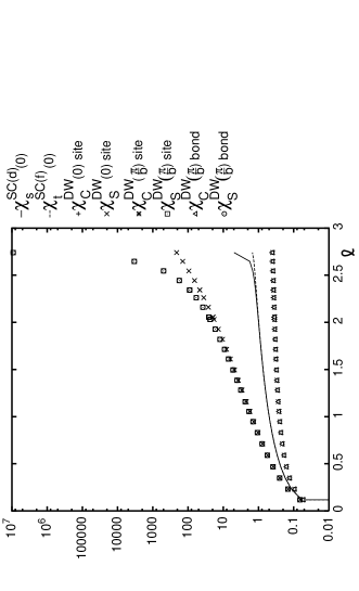
Figure 8: Flow of some susceptibilities, at $\tilde{U}=1$ and $2t_{\perp}/\Lambda_{0}=0.016$. $\chi\lower 1.6pt\hbox{${}^{{\rm SC}(d)}_{s}(0)$}$ is almost suppressed at $\Lambda_{c}$.

Hence, this result differs drastically from those obtained when the $k_{\|}$ dependence is neglected.

Moreover, we observe a transition between the SDW phase and the SC one, at a critical parameter $t_{\perp c}(U)$.

Critical behavior

We characterize this transition by different ways.

First of all, the behaviour of the renormalized two-particle couplings change very rapidly, at $t_{\perp c}(U)$: as $t_{\perp}$ decreases, $|\tilde{g}_{01}(\Lambda_{c})|$ and $|\tilde{g}_{02}(\Lambda_{c})|$ shrink suddenly, then, after a little interval, $\tilde{g}_{01}(\Lambda_{c})$ and $\tilde{g}_{02}(\Lambda_{c})$ become positive (and even $>\tilde{U}$, see on Fig. 7). We also observe changes, though less significant, for the other couplings $\tilde{g}$ (for instance, $|\tilde{g}_{f01}(\Lambda_{c})|$ decreases and $\tilde{g}_{b1}(\Lambda_{c})$ becomes negative when $t_{\perp}$ increases).

Moreover, we observe (on Fig. 9) a marked site/bond separation of the SDW susceptibility, at $t_{\perp c}(U)$. The site and bond SDW susceptibilities are degenerate for $t_{\perp}\leq t_{\perp c}(U)$ (in the SDW phase), which is consistent with the fact they should be equal at $t_{\perp}=0$ (where the system is purely one-dimensional, see Ref. [35]), while they smoothly separate after the transition. The same site/bond separation occurs for the CDW susceptibility.

Figure 9: Curves of $\chi\lower 1.6pt\hbox{${}^{{\rm SC}(d)}_{s}$}(\Lambda_{c})$ and $\chi^{\rm DW}_{S}(\Lambda_{c})$ versus $2t_{\perp}/\Lambda_{0}$.

Transition region

The behaviour of most of the parameters that we have examined indicates the same critical value $t_{\perp c}(U)$, which we have determined exactly, using the slope criterion.

However,$|\chi\lower 1.6pt\hbox{${}^{{\rm SC}(d)}_{s}$}(0)|<|\chi^{\rm DW}_{S}({\pi\over b})|$ holds until $t_{\perp}$ reaches a value $t_{\perp c2}(U)$; this second critical value, which corresponds to the height criterion, is confirmed by minor modifications of behaviour, which occur in the interval $t_{\perp c}(U)<t_{\perp}\leq t_{\perp c2}(U)$ and are very smooth (for instance, $\tilde{g}_{b1}(\Lambda_{c})$ and $\tilde{g}_{b2}(\Lambda_{c})$ cross) .

The numerical determination of $t_{\perp c2}(U)$ is very stable (see Fig.10), and the complete behaviour, from the SDW phase to the SC phase, is clear on Fig. 9, which shows the absolute values of the susceptibilities at $\Lambda_{c}$.

The region $t_{\perp c}(U)<t_{\perp}\leq t_{\perp c2}(U)$ is called transition region, we believe it is a superconducting phase, where SDW instabilities seem however to dominate. The SDW are precursor manifestations of the pure SDW phase, which is next to the transition region.

As already stated, our results converge very rapidly when the band width on which we project the momenta is increased. The complete phase diagram (for $C_{\rm back}=C_{\rm for}=0$) is shown on Fig. 10, for $n_{\rm max}=2,$ 3 and 4.

Figure 10: Phase diagram when the $k_{\|}$ dependence is included.

Moreover, it is most interesting to note that, contrary to the pure SDW phase, the transition region can be detected when the $k_{\|}$ dependence is neglected (the value of $t_{\perp c2}(U)$ is lowered). This can be seen, for instance, on Fig. 11, which corresponds to Fig. 9 with no $k_{\|}$ dependence.

Figure 11: Curves of $\chi\lower 1.6pt\hbox{${}^{(d)}_{s}$}(\Lambda_{c})$ and $\chi^{\rm DW}_{S}(\Lambda_{c})$ versus $2t_{\perp}/\Lambda_{0}$ when $k_{\|}$ is neglected.

SC critical temperature

The critical energy $\Lambda_{c}$ at which SC susceptibility diverges gives an approximate indication of the SC critical temperature. We give a plot of $\Lambda_{c}/\Lambda_{0}$ versus $2t_{\perp}/\Lambda_{0}$; as seen on Fig. 12, $\Lambda_{c}$ is roughly decreasing with $t_{\perp}$. The band gap parameter $t_{\perp}$ is also increasing with pressure; therefore, this behaviour is compatible with the experimental data, which show that $T_{c}$ is decreasing with pressure in quasi-one-dimensional organic compounds.

Figure 12: Curves of $\Lambda_{c}/\Lambda_{0}={\mathop{\,\rm e}}^{-\ell_{c}}$ versus $2t_{\perp}/\Lambda_{0}$ with $n_{\rm max}=2$ (a), $n_{\rm max}=3$ (b) and $n_{\rm max}=4$ (c).

b Discussion

As already mentioned, as soon as the dependence of $k_{\|}$ is included, we observe two separated phases, one purely SDW, the other one a SC phase with competing SDW instabilities.

On the other hand, for $t_{\perp}\geq 1$, i.e. when the initial bandwidth lies inside $[k_{f\pi},k_{f0}]$, the $k_{\|}$ dependence has no observable influence on the susceptibilities.

In the SDW phase, our results prove the existence of large antiferromagnetic fluctuations. We believe that these SDW instabilities are not the signature of a localized antiferromagnetic ground state, but of antiferromagnetic itinerant electrons, as it is indeed observed in Bechgaard salts. Actually, the flow is driving towards a fixed point, which does not seem to be the one-dimensional solution : for instance, the renormalized couplings $\tilde{g}_{1}$ and $\tilde{g}_{2}$ of the 1-$d$ solution are 0 and 1/2 and differ from the values which we obtain when the flow is diverging, in the SDW phase (see Fig. 7 (a)).

We induce that the spin-gap should disappear in this SDW region, which is consistent with what Park and Kishine[24, 23] claim.

In the SC phase, the SC divergence is due to the Cooper channel, while that of density waves is due to the Peierls one (see, in the case of a single band model, Refs. [36, 32]). The appearance of $d$-wave superconductivity in ladder systems is well understood within a strong coupling scenario, where a spin gap leads to interchain Cooper pairing. However, in our calculations, we see that superconducting correlations are always enhanced by SDW fluctuations. Contrary to what Lee et al. claimed first[37], there is an itinerant electron mechanism in this case, which is the weak coupling equivalent of the localized electron mechanism in the strong electron scenario. It was proposed by Emery[38], and is essentially the spin analog of Kohn-Luttinger superconductivity. The mutual enhancement of the two channels is also discussed in Refs. [33, 39].

As a consequence of this mutual enhancement, the spin-gap should not appear with the first appearance of SC instabilities, but for somehow larger values of $t_{\perp}$.

Moreover, we observe that the SC pairing is a $\bf Q=0$ mechanism, while the SDW are excited by ${\bf Q}=(2\Delta k_{f},{\pi\over b})$ vectors. This can be explained by the symmetry of each channel. The Green function of the Cooper channel gives a factor $1/(\epsilon({\bf k})+\epsilon(-{\bf k}))$ and is minimized with the ${\bf k}\mapsto-{\bf k}$ symmetry, which corresponds to an intraband process. The Green function of the Peierls channel gives a factor $1/(\epsilon({\bf k})+\epsilon({\bf k+Q}))$ and is minimized with the ${\bf k}\mapsto{\bf k+Q}$ symmetry, which corresponds to an interband process.

This can also be seen in the RG equations. $d\ln(z^{\rm SC}(0))/d\ell$ depends only on $g_{0}$ and $g_{t}$, whereas $d\ln(z^{\rm SC}({\pi\over b}))/d\ell$ depends on $g_{f}$ and $g_{b}$. Since $g_{b}$ processes are depressed as soon as $\Lambda\leq 2t_{\perp}$, 0-condensate are favored. Moreover, this predominance is stabilized by the $dg_{t}/d\ell$ equations, in which the Cooper term depends on $g_{0}$, and by the $dg_{b}/d\ell$ equations, in which the Cooper term depends on $g_{f}$.

The same argument applies for DW instabilities. $d\ln(z^{\rm DW}(0))/d\ell$ depends on $g_{0}$ and $g_{b}$, whereas $d\ln(z^{\rm DW}({\pi\over b}))/d\ell$ depends on $g_{f}$ and $g_{t}$. So, $\pi$-processes are favored. Again, this is stabilized by the $dg_{t}/d\ell$ equations, in which the Peierls term depends on $g_{f}$, and by the $dg_{b}/d\ell$ equations, in which the Peierls term depends on $g_{0}$.

The critical temperature, in the SC phases, is indicated in Fig. 12. We chose $\tilde{U}=0.6$ in order to avoid the SDW phase. The general trend is that of a quasi-one-dimensional system; the increasing curve, for small values of $t_{\perp}$, can be related to transition effect and to the furthered influence of the SDW fluctuations.

6 Phase diagram with initial Coulombian interchain scattering

a Results

a.1 Influence of a backward interchain scattering

Let us now study the effect of a backward interchain scattering. This type of coupling has been inverstigated by Bourbonnais et al.[29] in the context of correlated quasi-onde-dimensional metals, for which CDW correlations are enhanced and triplet superconducting instabilities can occur. When the parameter $\tilde{C}_{\rm back}$ is increased, the behaviour of the susceptibilities depends on the parameters $(t_{\perp},\tilde{U})$.

Appearance of triplet SC and CDW

For $t_{\perp}\leq t_{\perp c}(U)$, the SDW phase exists for $\tilde{C}_{\rm back}$ small enough. As $\tilde{C}_{\rm back}$ is further increased, the SDW instabilities are replaced by CDW ones. The transition is smooth, and there is a narrow region where both SDW and CDW coexist (region $\bigcirc 3\;$ in Fig. 16). We show a $2t_{\perp}/\Lambda_{0}=0.01$ section of the susceptibilities at $\Lambda_{c}$ on Fig. 13.

Figure 13: Curves of the $\chi(\Lambda_{c})$ versus $\tilde{C}_{\rm back}$, at $\tilde{U}=1$ and a) $2t_{\perp}/\Lambda_{0}=0.01$; b) $2t_{\perp}/\Lambda_{0}=0.1$.

For $t_{\perp}\geq t_{\perp c}(U)$, the SC phase (with SC singlet $d$ and SDW instabilities) exists for $\tilde{C}_{\rm back}$ small enough. As $\tilde{C}_{\rm back}$ is further increased, the singlet SC modes are replaced by triplet ones, while SDW are replaced by CDW. Singlet and triplet SC appear to be antagonistic, and the transition is very pronounced; in the coexistence line between them, one also finds SDW and CDW divergences (see Fig. 14). On the contrary, the transition between SDW and CDW is very smooth, although the coexistence region is still narrow (region $\bigcirc 2\;$ in Fig. 16). We show a $2t_{\perp}/\Lambda_{0}=0.1$ section of the susceptibilities at $\Lambda_{c}$ on Fig. 13.

Figure 14: Flow of the susceptibilities for $2t_{\perp}/\Lambda_{0}=0.32$ and $\tilde{C}_{\rm back}=0.18$.

The triplet SC condensate has $f_{x}$ symmetry. The corresponding susceptibility is mostly divergent in a region of coexistence with SDW and CDW (region $\bigcirc 2\;$ in Fig. 16), but it is also divergent in a region of coexistence with only CDW (region $\bigcirc 1\;$ in Fig. 16).

When $\tilde{C}_{\rm back}$ is large enough, the triplet SC modes are suppressed, and the region is a pure CDW phase. We show a section of the susceptibilities at $\Lambda_{c}$, for $\tilde{C}_{\rm back}=0.2$ and $\tilde{C}_{\rm back}=0.3$, on Fig. 15, which clearly indicates the domain of existence of the triplet SC.

Figure 15: Curves of the susceptibilities $\chi(\Lambda_{c})$ versus $2t_{\perp}/\Lambda_{0}$, for : a) $\tilde{C}_{\rm back}=0.4$; b) $\tilde{C}_{\rm back}=0.6$.

Site/bond separation

As we have already observed it, in the case of $C_{\rm back}=C_{\rm for}=0$, for small values of $t_{\perp}$, site and bond SDW susceptibilities are degenerate, as well as site and bond CDW ones.

This generalizes for all values of $\tilde{C}_{\rm back}$. The site/bond separation line is an increasing function $t_{\perp g}(C_{\rm back})$ of $C_{\rm back}$, shown on Fig. 16; For small values of $U$, this line crosses the SC domain, but for $\tilde{U}=1$ it is already disconnected from the SC frontier (although it remains close to it).

Figure 16: Phase diagram for $\tilde{U}=1$. The shaded area indicates the divergence of the triplet susceptibility. The dashed line separates site/bond degenerated states (below) and non degenerated ones (above). Other lines and domains are explained in the legend or in the text.

a.2 Influence of a forward interchain scattering

The phase diagram when $C_{\rm for}$ is included is very rich, and beyond the scope of this article.

We would like to emphasize only the fact that all SC instabilities are suppressed when $C_{\rm for}$ is increased. Fig. 17 gives a typical flow of the susceptibilities, with a large $\tilde{C}_{\rm for}$.

Figure 17: Flow of the susceptibilities, $t_{\perp}=0.02$ and : $\tilde{C}_{\rm for}=0.95$.

b Discussion

Let us analyze these behaviors, which follow simple trends.

The CDW instabilities are enhanced when $g_{C}$ is increased, whereas SDW ones are enhanced when $g_{S}$ is increased (this can be verified in the corresponding RG equations of B.2). Similarly, singlet SC instabilities are enhanced when $g_{s}$ is increased, whereas triplet ones are enhanced when $g_{t}$ is increased.

So, an increase of $C_{\rm back}$ implies an increase of the real space coupling $g_{1}$, and thus, from Eq. (5), it favors CDW instabilities against SDW ones, and from Eq. (4), it favors triplet SC instabilities and depresses singlet SC ones.

Similarly, an increase of $C_{\rm for}$ implies an increase of the real space coupling $g_{2}$, and thus, from Eq. (5), it favors CDW and SDW instabilities, and from Eq. (4), it depresses SC ones.

Of course, we examine here the influence of parameters $C_{\rm back}$ and $C_{\rm back}$ on the bare couplings. However, we believe that the flow could not just simply reverse this influence, even if the renormalized values of the couplings differ a lot from their bare values. Moreover, one verifies that these conclusions exactly correspond to the observed behaviour.

The density wave interactions are on site, whereas the SC pairing are inter-site (except for singlet $s$ one), so we believe that the DW instabilities appear first, and then enhance the SC ones. This is not true of the DW bond correlations, but we observed no divergences of these ones, and we have not studied any other sophisticated inter-site DW excitation response.

From this point of view, the fact that $\pi$ DW processes are favored, as we already discussed before, implies a $\pi$ dephasing between both chains of the ladder. The $\pi$ dephasing of the SDW thus fits perfectly singlet $d$ condensate (which consists in a pairing of two electrons on a rung, with opposite spins, see Fig. 3 (b)). This accounts nicely for the appearance of singlet SC instability, induced by SDW one.

In the same trend of ideas, the $\pi$ dephasing of the CDW fits triplet $f_{x}$ condensate (which consists in a pairing of two electrons on each chain, one stepped by unity from the other, see Fig. 4 (a)) and accounts for the appearance of triplet SC instability, induced by CDW one.

On the contrary, the triplet $p_{x}$ condensate consists in two following electrons on one chain (see Fig. 4 (b)), this pairing is not enhanced by CDW instabilities; in fact, it is the analog of singlet $s$ condensate, which is not either enhanced by SDW instabilities, and is therefore disadvantaged, compared to $d$ pairing.

As can be observed on Fig. 4, triplet $f_{x}$ condensate are not incompatible with CDW. For instance, one could easily figure out a succession of condensate, with alternate spins, inducing back a global modulation of the chains. A similar scenario is not possible with triplet $p$ condensate.

One should be aware that the symmetry classification we have used is very specific of the ladder system, and could not be extended to an infinite number of chains. The difference between $p$ and $f$ condensate is very subtle and the situation could reveal quite different in the general quasi-one-dimensional systems.

7 Conclusion

We have investigated the phase diagram of a ladder system, in the Hubbard model, with an interchain coupling $t_{\perp}$, using functional RG method, in the OPI scheme. We have introduced an original parameterization of the $k_{\|}$ dependence, and obtained rather new results, in particular, we have proved the existence of a new phase with only SDW fluctuations, for small enough values of $t_{\perp}$. From the divergences of the scattering couplings, we induce that this phase is different from the one-dimensional solution. However, for very small values of $t_{\perp}$ ($t_{\perp}<\Lambda_{0}10^{-4}$), we find the usual one-dimensional behaviour.

Our results altogether prove that the $k_{\|}$ dependence is important and must be taken into account in such a ladder system. The fact that this variables become influential in a ladder does not mean that the corresponding couplings $g(2\Delta k_{f},-2\Delta k_{f},0)$, etc., are relevant. In fact, if the cut-off $\Lambda\to 0$, these couplings are left out of the integrated band, so they could only be marginal[28]. However, the divergence takes place at $\Lambda_{c}$, which is of the order of $\Delta k_{f}$, and this explains why these couplings, which are shifted by $\pm 2\Delta k_{f}$ from the Fermi points, have a non trivial behaviour and have to be taken into account. Moreover, as already explained in b.1, during the flow, these couplings influence those, with all momenta at the Fermi points, until $\Lambda=2\Delta k_{f}$. This influence is still sensitive, when the divergence takes place. This explains why we could distinguish a new phase, which has not yet been observed by usual methods.

When $t_{\perp}$ is very large, however (for instance, $t_{\perp}\sim\Lambda_{0}$), the flow continues up to $\Lambda_{c}\ll v_{f}\Delta k_{f}$ (otherwise, the integrated band would not vary much and the renormalized couplings neither differ much from their bare values), and the above argument applies, proving that couplings $g(2\Delta k_{f},-2\Delta k_{f},0)$, etc., are marginal or irrelevant. In that case, $k_{\|}$ are not influential, and our results coincide indeed with former calculations.

We have also given a detailed classification of the response function, which provides a convenient tool for the determination of order parameters and of related susceptibilities, corresponding to different instability processes.

We are proceeding now to a complete study of the long range correlations, and in particular, of the uniform susceptibility. This task however proves quite difficult, because of the $k_{\|}$ dependence, which has to be carefully taken into account. We expect that the spin-gap will indeed disappear in the SDW phase we have brought to evidence.

We have also investigated the influence of interchain scattering, and showed that a backward interchain scattering can raise triplet superconductivity, a resulst consistent with the conclusions of a previous work by Bourbonnais et al.[29, 30] on correlated quasi-one-dimensional metals. The appearance of triplet SC in a ladder is a very exciting and promising result, since various authors[40, 41] claim to have found experimental evidence of these instabilities. Even the narrowness of the triplet SC existence region seems to fit the experimental data, which report high sensitivity of these fluctuations to some key parameters. This work gains to be compared with the previous work of Varma et al., who did similar investigations[42].

We would like to thank N. Dupuis, S. Haddad and B. Douçot for fruitful discussions and advices. J. C. Nickel wishes to thank the Gottlieb Daimler- und Karl Benz-Stiftung for partial support.

Appendix

A Couplings

A.1 Two-particle couplings

Here are the definitions of the different couplings $g$, from the two-particle parameter $\cal G$, and the corresponding diagrams.

$$\begin{array}[]{c}g_{0}(p_{1},p_{2},p^{\prime}_{2},p^{\prime}_{1})=\\ {\cal G}(k_{f0}+p_{1},-k_{f0}+p_{2},-k_{f0}+p^{\prime}_{2},k_{f0}+p^{\prime}_{1})\\ g_{\pi}(p_{1},p_{2},p^{\prime}_{2},p^{\prime}_{1})=\\ {\cal G}(k_{f\pi}+p_{1},-k_{f\pi}+p_{2},-k_{f\pi}+p^{\prime}_{2},k_{f\pi}+p^{\prime}_{1})\\ g_{\!f0}(p_{1},p_{2},p^{\prime}_{2},p^{\prime}_{1})=\\ {\cal G}(k_{f0}+p_{1},-k_{f\pi}+p_{2},-k_{f\pi}+p^{\prime}_{2},k_{f0}+p^{\prime}_{1})\\ g_{\!f\pi}(p_{1},p_{2},p^{\prime}_{2},p^{\prime}_{1})=\\ {\cal G}(k_{f\pi}+p_{1},-k_{f0}+p_{2},-k_{f0}+p^{\prime}_{2},k_{f\pi}+p^{\prime}_{1})\\ g_{t0}(p_{1},p_{2},p^{\prime}_{2},p^{\prime}_{1})=\\ {\cal G}(k_{f0}+p_{1},-k_{f0}+p_{2},-k_{f\pi}+p^{\prime}_{2},k_{f\pi}+p^{\prime}_{1})\\ g_{t\pi}(p_{1},p_{2},p^{\prime}_{2},p^{\prime}_{1})=\\ {\cal G}(k_{f\pi}+p_{1},-k_{f\pi}+p_{2},-k_{f0}+p^{\prime}_{2},k_{f0}+p^{\prime}_{1})\\ g_{b0}(p_{1},p_{2},p^{\prime}_{2},p^{\prime}_{1})=\\ {\cal G}(k_{f0}+p_{1},-k_{f\pi}+p_{2},-k_{f0}+p^{\prime}_{2},k_{f\pi}+p^{\prime}_{1})\\ g_{b\pi}(p_{1},p_{2},p^{\prime}_{2},p^{\prime}_{1})=\\ {\cal G}(k_{f\pi}+p_{1},-k_{f0}+p_{2},-k_{f\pi}+p^{\prime}_{2},k_{f0}+p^{\prime}_{1})\end{array}$$

Figure 18: Schematic definitions of the couplings $g$

The relations between the different representations can be found in Refs. [27] or [43]. Here, they reduce to : $$\begin{array}[]{rcl}g_{s}&=&-g_{1}-g_{2}\\ g_{t}&=&g_{1}-g_{2}\end{array}$$ (4) $$\begin{array}[]{rcl}g_{C}&=&g_{2}-2g_{1}\\ g_{S}&=&g_{2}\end{array}$$ (5)

A.2 Other couplings

Here are the definitions of the different couplings $z$, from the couplings to external fields $\cal Z$.

We omit the spin index $\alpha$ nor the symmetry index $\Gamma$, and use the notation explained further in appendix C.1. Mind that $\Gamma=s,d,g\;$ for $\alpha=s$ (singlet) and $\Gamma=p,f$ for $\alpha=t$ (triplet). The symmetry ($s$, $d_{x^{2}-y^{2}}$, $g$, $p_{x}$, $f_{x}$ or $f_{y}$) applying to each one is detailed in the main text.

$$\begin{array}[]{c}z^{\rm SC}_{0}(p_{1},p_{2},q)=\\ {\cal Z}^{\rm SC}(-k_{f0}+p_{1},k_{f0}+p_{2},(q,0),0)\\ z^{\rm SC}_{\pi}(p_{1},p_{2},q)=\\ {\cal Z}^{\rm SC}(-k_{f\pi}+p_{1},k_{f\pi}+p_{2},(q,0),\pi)\\ z^{\rm SC}_{+}(p_{1},p_{2},q)=\\ {\cal Z}^{\rm SC}(-k_{f\pi}+p_{1},k_{f0}+p_{2},(q,{\pi\over b}),0)\\ z^{\rm SC}_{-}(p_{1},p_{2},q)=\\ {\cal Z}^{\rm SC}(-k_{f0}+p_{1},k_{f\pi}+p_{2},(q,{\pi\over b}),\pi)\\ z^{\rm DW}_{0}(p_{1},p_{2},q)=\\ {\cal Z}^{\rm DW}(-k_{f0}+p_{1},k_{f0}+p_{2},(q-2k_{f0},0),0)\\ z^{\rm DW}_{\pi}(p_{1},p_{2},q)=\\ {\cal Z}^{\rm DW}(-k_{f\pi}+p_{1},k_{f\pi}+p_{2},(q-2k_{f\pi},0),\pi)\\ z^{\rm DW}_{+}(p_{1},p_{2},q)=\\ {\cal Z}^{\rm DW}(-k_{f\pi}+p_{1},k_{f0}+p_{2},(q-k_{f0}-k_{f\pi},{\pi\over b}),0)\\ z^{\rm DW}_{-}(p_{1},p_{2},q)=\\ {\cal Z}^{\rm DW}(-k_{f0}+p_{1},k_{f\pi}+p_{2},(q-k_{f0}-k_{f\pi},{\pi\over b}),\pi)\end{array}$$

Figure 19: Schematic definitions of the couplings $z$

B RG equations

We give here the detailed RG equations.

B.1 $g$ couplings

Here are the RG equations for the couplings $g$, in $(c,l,p)$ representation.

The spin dependence is given, for all terms, by

$${dg_{\alpha}\over d\ell}=\sum_{\beta,\gamma}g_{\beta}\left({\cal C}^{\beta\gamma}_{\alpha}+{\cal P}^{\beta\gamma}_{\alpha}\right)g_{\gamma}$$

where $\cal C$ and $\cal P$ correspond, respectively, to the Cooper and Peierls channels, and are given, in the g-ology representation, by

$${\cal C}_{1}=-\pmatrix{0&1\cr 1&0\cr}\quad{\cal C}_{2}=-\pmatrix{1&0\cr 0&1\cr}\quad$$

$${\cal P}_{1}=\pmatrix{2&-1\cr-1&0\cr}\quad{\cal P}_{2}=\pmatrix{0&0\cr 0&-1\cr}\ ,$$

see, for instance, Refs. [44, 27, 43]. In the following equations, all two first terms are Cooper ones, whereas all two last terms are Peierls ones; so, we omit the spin dependence, which is given by the above equations, for each term. One gets

$$\begin{array}[]{l}\qquad\qquad{\displaystyle{d\tilde{g}_{0}\over d\ell}}(c,l,p)=\\ {\Lambda\over 8\Lambda+4|c|}\Big{(}\sum\limits_{\pm}\tilde{g}_{0}({\scriptstyle c,\pm(\Lambda+{|c|\over 2})+{l+p\over 2},\mp(\Lambda+{|c|\over 2})+{l+p\over 2}})\tilde{g}_{0}({\scriptstyle c,\mp(\Lambda+{|c|\over 2})+{l-p\over 2},\mp(\Lambda+{|c|\over 2})-{l-p\over 2}})\\ +\sum\limits_{\pm}\tilde{g}_{t0}({\scriptstyle c,\pm(\Lambda+{|c|\over 2})+{l+p\over 2},\mp(\Lambda+{|c|\over 2})+{l+p\over 2}})\tilde{g}_{t\pi}({\scriptstyle c,\mp(\Lambda+{|c|\over 2})+{l-p\over 2},\mp(\Lambda+{|c|\over 2})-{l-p\over 2}})\Big{)}\\ +{\Lambda\over 8\Lambda+4|p|}\Big{(}\sum\limits_{\pm}\tilde{g}_{0}({\scriptstyle\mp(\Lambda+{|p|\over 2})+{c+l\over 2},\pm(\Lambda+{|p|\over 2})+{c+l\over 2},p})\tilde{g}_{0}({\scriptstyle\mp(\Lambda+{|p|\over 2})+{c-l\over 2},\mp(\Lambda+{|p|\over 2})-{c-l\over 2},p})\Big{)}\\ +{\Lambda\over 8\Lambda+4|p+2\Delta k_{f}|}\Big{(}\sum\limits_{\pm}\tilde{g}_{b0}({\scriptstyle\mp(\Lambda+{|p+2\Delta k_{f}|\over 2})+{c+l\over 2}-\Delta k_{f},\pm(\Lambda+{|p+2\Delta k_{f}|\over 2})+{c+l\over 2}-\Delta k_{f},p})\\ \lx@intercol\hfil\tilde{g}_{b\pi}({\scriptstyle\mp(\Lambda+{|p+2\Delta k_{f}|\over 2})+{c-l\over 2}+\Delta k_{f},\mp(\Lambda+{|p+2\Delta k_{f}|\over 2})-{c-l\over 2}+\Delta k_{f},p+2\Delta k_{f}})\Big{)}\lx@intercol\end{array}$$

$$\begin{array}[]{l}\qquad\qquad{\displaystyle{d\tilde{g}_{\!f0}\over d\ell}}(c,l,p)=\\ {\Lambda\over 8\Lambda+4|c|}\Big{(}\sum\limits_{\pm}\tilde{g}_{\!f0}({\scriptstyle c,\pm(\Lambda+{|c|\over 2})+{l+p\over 2},\mp(\Lambda+{|c|\over 2})+{l+p\over 2}})\tilde{g}_{\!f0}({\scriptstyle c,\mp(\Lambda+{|c|\over 2})+{l-p\over 2},\mp(\Lambda+{|c|\over 2})-{l-p\over 2}})\Big{)}\\ +{\Lambda\over 8\Lambda+4|c+2\Delta k_{f}|}\Big{(}\sum\limits_{\pm}\tilde{g}_{b0}({\scriptstyle c,\pm(\Lambda+{|c+2\Delta k_{f}|\over 2})+{l+p\over 2}-\Delta k_{f},\mp(c\Lambda+{|c+2\Delta k_{f}|\over 2})+{l+p\over 2}-\Delta k_{f}})\\ \lx@intercol\hfil\tilde{g}_{b\pi}({\scriptstyle c+2\Delta k_{f},\mp(\Lambda+{|c+2\Delta k_{f}|\over 2})+{l-p\over 2}+\Delta k_{f},\mp(\Lambda+{|c+2\Delta k_{f}|\over 2})-{l-p\over 2}}+\Delta k_{f})\Big{)}\lx@intercol\\ +{\Lambda\over 8\Lambda+4|p|}\Big{(}\sum\limits_{\pm}\tilde{g}_{\!f0}({\scriptstyle\mp(\Lambda+{|p|\over 2})+{c+l\over 2},\pm(\Lambda+{|p|\over 2})+{c+l\over 2},p})\tilde{g}_{\!f0}({\scriptstyle\mp(\Lambda+{|p|\over 2})+{c-l\over 2},\mp(\Lambda+{|p|\over 2})-{c-l\over 2},p})\\ +\sum\limits_{\pm}\tilde{g}_{t0}({\scriptstyle\mp(\Lambda+{|p|\over 2})+{c+l\over 2},\pm(\Lambda+{|p|\over 2})+{c+l\over 2},p})\tilde{g}_{t\pi}({\scriptstyle\mp(\Lambda+{|p|\over 2})+{c-l\over 2},\mp(\Lambda+{|p|\over 2})-{c-l\over 2},p})\Big{)}\end{array}$$

$$\begin{array}[]{l}\qquad\qquad{\displaystyle{d\tilde{g}_{t0}\over d\ell}}(c,l,p)=\\ {\Lambda\over 8\Lambda+4|c|}\Big{(}\sum\limits_{\pm}\tilde{g}_{0}({\scriptstyle c,\pm(\Lambda+{|c|\over 2})+{l+p\over 2},\mp(\Lambda+{|c|\over 2})+{l+p\over 2}})\tilde{g}_{t0}({\scriptstyle c,\mp(\Lambda+{|c|\over 2})+{l-p\over 2},\mp(\Lambda+{|c|\over 2})-{l-p\over 2}})\\ +\sum\limits_{\pm}\tilde{g}_{t0}({\scriptstyle c,\pm(\Lambda+{|c|\over 2})+{l+p\over 2},\mp(\Lambda+{|c|\over 2})+{l+p\over 2}})\tilde{g}_{\pi}({\scriptstyle c,\mp(\Lambda+{|c|\over 2})+{l-p\over 2},\mp(\Lambda+{|c|\over 2})-{l-p\over 2}})\Big{)}\\ +{\Lambda\over 8\Lambda+4|p|}\Big{(}\sum\limits_{\pm}\tilde{g}_{t0}({\scriptstyle\mp(\Lambda+{|p|\over 2})+{c+l\over 2},\pm(\Lambda+{|p|\over 2})+{c+l\over 2},p})\tilde{g}_{\!f\pi}({\scriptstyle\mp\Lambda+{|p|\over 2})+{c-l\over 2},\mp(\Lambda+{|p|\over 2})-{c-l\over 2},p})\\ +\sum\limits_{\pm}\tilde{g}_{\!f0}({\scriptstyle\mp(\Lambda+{|p|\over 2})+{c+l\over 2},\pm(\Lambda+{|p|\over 2})+{c+l\over 2},p})\tilde{g}_{t0}({\scriptstyle\mp(\Lambda+{|p|\over 2})+{c-l\over 2},\mp(\Lambda+{|p|\over 2})-{c-l\over 2},p})\Big{)}\end{array}$$

$$\begin{array}[]{l}\qquad\qquad{\displaystyle{d\tilde{g}_{b0}\over d\ell}}(c,l,p)=\\ {\Lambda\over 8\Lambda+4|c|}\Big{(}\sum\limits_{\pm}\tilde{g}_{\!f0}({\scriptstyle c,\pm(\Lambda+{|c|\over 2})+{l+p\over 2}+\Delta k_{f},\mp(\Lambda+{|c|\over 2})+{l+p\over 2}+\Delta k_{f}})\tilde{g}_{b0}({\scriptstyle c,\mp(\Lambda+{|c|\over 2})+{l-p\over 2}-\Delta k_{f},\mp(\Lambda+{|c|\over 2})-{l-p\over 2}-\Delta k_{f}})\Big{)}\\ +{\Lambda\over 8\Lambda+4|c+2\Delta k_{f}|}\Big{(}\sum\limits_{\pm}\tilde{g}_{b0}({\scriptstyle c,\pm(\Lambda+{|c+2\Delta k_{f}|\over 2})+{l+p\over 2},\mp(\Lambda+{|c+2\Delta k_{f}|\over 2})+{l+p\over 2}})\tilde{g}_{\!f\pi}({\scriptstyle c+2\Delta k_{f},\mp(\Lambda+{|c+2\Delta k_{f}|\over 2}){l-p\over 2},\mp(\Lambda+{|c+2\Delta k_{f}|\over 2})-{l-p\over 2}})\Big{)}\\ +{\Lambda\over 8\Lambda+4|p|}\Big{(}\sum\limits_{\pm}\tilde{g}_{0}({\scriptstyle\mp(\Lambda+{|p|\over 2})+{c+l\over 2}+\Delta k_{f},\pm(\Lambda+{|p|\over 2})+{c+l\over 2}+\Delta k_{f},p})\tilde{g}_{b0}({\scriptstyle\mp(\Lambda+{|p|\over 2})+{c-l\over 2}-\Delta k_{f},\mp(\Lambda+{|p|\over 2})-{c-l\over 2}-\Delta k_{f},p})\Big{)}\\ +{\Lambda\over 8\Lambda+4|p+2\Delta k_{f}|}\Big{(}\sum\limits_{\pm}\tilde{g}_{b0}({\scriptstyle\mp(\Lambda+{|p+2\Delta k_{f}|\over 2})+{c+l\over 2},\pm(\Lambda+{|p+2\Delta k_{f}|\over 2})+{c+l\over 2},p})\tilde{g}_{\pi}({\scriptstyle\mp(\Lambda+{|p+2\Delta k_{f}|\over 2})+{c-l\over 2},\mp(\Lambda+{|p+2\Delta k_{f}|\over 2})-{c-l\over 2},p+2\Delta k_{f}})\Big{)}\end{array}$$

B.2 $z$ couplings

Here are the RG equations for the couplings $z$, in $(k,c,p)$ representation. The $z^{\rm SC}$ couplings should be written in the singlet/triplet representation ($\alpha=s,t$), and the $z^{\rm DW}$ couplings should be written in the Charge/Spin representation ($\alpha=C,S$). Then, the spin dependence simply writes, for each one

$${dz_{\alpha}\over d\ell}=g_{\alpha}z_{\alpha}$$

and will therefore be again omitted. One gets

$$\begin{array}[]{l}\qquad\qquad{\displaystyle{dz^{\rm SC}_{0}\over d\ell}}(c,k)={\Lambda\over 4\Lambda+2|c|}\Big{(}\sum\limits_{\pm}\tilde{g}_{0}({\scriptstyle c,\pm(\Lambda+{|c|\over 2})+{c\over 2}-k,\mp(\Lambda+{|c|\over 2})+{c\over 2}-k})z^{\rm SC}_{0}({\scriptstyle c,\pm(\Lambda+{|c|\over 2})+{c\over 2}})\\ \lx@intercol\hfil+\sum\limits_{\pm}\tilde{g}_{t0}({\scriptstyle c,\pm(\Lambda+{|c|\over 2})+{c\over 2}-k,\mp(\Lambda+{|c|\over 2})+{c\over 2}-k})z^{\rm SC}_{\pi}({\scriptstyle c,\pm(\Lambda+{|c|\over 2})+{c\over 2}})\Big{)}\lx@intercol\end{array}$$

$$\begin{array}[]{l}\qquad\qquad{\displaystyle{dz^{\rm SC}_{+}\over d\ell}}(c,k)={\Lambda\over 4\Lambda+2|c|}\sum\limits_{\pm}\tilde{g}_{f0}({\scriptstyle c,\pm(\Lambda+{|c|\over 2})+{c\over 2}-k,\mp(\Lambda+{|c|\over 2})+{c\over 2}-k})z^{\rm SC}_{+}({\scriptstyle c,\pm(\Lambda+{|c|\over 2})+{c\over 2}})\\ +{\Lambda\over 4\Lambda+2|c+2\Delta k_{f}|}\sum\limits_{\pm}\tilde{g}_{b0}({\scriptstyle c,\pm(\Lambda+{|c+2\Delta k_{f}|\over 2})+{c\over 2}-\Delta k_{f}-k,\mp(\Lambda+{|c+2\Delta k_{f}|\over 2})+{c\over 2}-\Delta k_{f}-k})z^{\rm SC}_{-}({\scriptstyle c+2\Delta k_{f},\pm(\Lambda+{|c+2\Delta k_{f}|\over 2})+{c\over 2}+\Delta k_{f}})\end{array}$$

$$\begin{array}[]{l}\qquad\qquad{\displaystyle{dz^{\rm DW}_{0}\over d\ell}}(p,k)={\Lambda\over 4\Lambda+2|p|}\sum\limits_{\pm}\tilde{g}_{0}({\scriptstyle\pm(\Lambda+{|p|\over 2})+{p\over 2}+k,\pm(\Lambda+{|p|\over 2})-{p\over 2}-k,p})z^{\rm DW}_{0}({\scriptstyle p,\pm(\Lambda+{|p|\over 2})-{p\over 2}})\\ \!\!\!\!\!\!\!\!+{\Lambda\over 4\Lambda+2|p+2\Delta k_{f}|}\sum\limits_{\pm}\tilde{g}_{b\pi}({\scriptstyle\pm(\Lambda+{|p+2\Delta k_{f}|\over 2})+{p\over 2}+\Delta k_{f}+k,\pm(\Lambda+{|p+2\Delta k_{f}|\over 2})-{p\over 2}+\Delta k_{f}-k,p+2\Delta k_{f}})z^{\rm DW}_{\pi}({\scriptstyle p+2\Delta k_{f},\pm(\Lambda+{|p+2\Delta k_{f}|\over 2})-{p\over 2}-\Delta k_{f}})\end{array}$$

$$\begin{array}[]{l}\qquad\qquad{\displaystyle{dz^{\rm DW}_{+}\over d\ell}}(p,k)={\Lambda\over 4\Lambda+2|p|}\Big{(}\sum\limits_{\pm}\tilde{g}_{f0}({\scriptstyle\pm(\Lambda+{|p|\over 2})+{p\over 2}+k,\pm(\Lambda+{|p|\over 2})-{p\over 2}-k,p})z^{\rm DW}_{+}({\scriptstyle p,\pm(\Lambda+{|p|\over 2})-{p\over 2}})\\ \lx@intercol\hfil+\sum\limits_{\pm}\tilde{g}_{t\pi}({\scriptstyle\pm(\Lambda+{|p|\over 2})+{p\over 2}+k,\pm(\Lambda+{|p|\over 2})-{p\over 2}-k,p})z^{\rm DW}_{-}({\scriptstyle p,\pm(\Lambda+{|p|\over 2})-{p\over 2}})\Big{)}\lx@intercol\end{array}$$

B.3 $\chi$ couplings

Here are the RG equations for the susceptibilities $\chi$, with the same spin dependence as the corresponding $z$ couplings, which is again omitted,

$$\begin{array}[]{l}\qquad\qquad{\displaystyle{d\chi^{\rm SC}_{0}\over d\ell}}(q)=-{\Lambda\over 4\Lambda+2|q|}\Big{(}\sum\limits_{\pm}z^{\rm SC}_{0}({\scriptstyle q,\pm(\Lambda+{|q|\over 2})+{q\over 2}})^{2}+\sum\limits_{\pm}z^{\rm SC}_{\pi}({\scriptstyle q,\pm(\Lambda+{|q|\over 2})+{q\over 2}})^{2}\Big{)}\end{array}$$

$$\begin{array}[]{l}\qquad\qquad{\displaystyle{d\chi^{\rm SC}_{+}\over d\ell}}(q)=-{\Lambda\over 4\Lambda+2|q|}\sum\limits_{\pm}z^{\rm SC}_{+}({\scriptstyle q,\pm(\Lambda+{|q|\over 2})+{q\over 2}})^{2}-{\Lambda\over 4\Lambda+2|q+2\Delta k_{f}|}\sum\limits_{\pm}z^{\rm SC}_{-}({\scriptstyle q+2\Delta k_{f},\pm(\Lambda+{|q+2\Delta k_{f}|\over 2})+{q\over 2}+\Delta k_{f}})^{2}\end{array}$$

$$\begin{array}[]{l}\!\!\!\!\!\!\qquad\qquad{\displaystyle{d\chi^{\rm DW}_{0}\over d\ell}}(q)=-{\Lambda\over 4\Lambda+2|q|}\sum\limits_{\pm}z^{\rm DW}_{0}({\scriptstyle-q,\pm(\Lambda+{|q|\over 2})+{q\over 2}})^{2}-{\Lambda\over 4\Lambda+2|q-2\Delta k_{f}|}\sum\limits_{\pm}z^{\rm DW}_{\pi}({\scriptstyle-q+2\Delta k_{f},\pm(\Lambda+{|q-2\Delta k_{f}|\over 2})+{q\over 2}-\Delta k_{f}})^{2}\end{array}$$

$$\begin{array}[]{l}\qquad\qquad{\displaystyle{d\chi^{\rm DW}_{+}\over d\ell}}(q)=-{\Lambda\over 4\Lambda+2|q|}\Big{(}\sum\limits_{\pm}z^{\rm DW}_{+}({\scriptstyle-q,\pm(\Lambda+{|q|\over 2})+{q\over 2}})^{2}+\sum\limits_{\pm}z^{\rm DW}_{-}({\scriptstyle-q,\pm(\Lambda+{|q|\over 2})+{q\over 2}})^{2}\Big{)}\end{array}$$

C Symmetries

C.1 Ordinary symmetries

If we apply the conjugation symmetry $C$ to the two-particle coupling $\cal G$, we get :

$${\cal G}(P^{\prime}_{1},P^{\prime}_{2},P_{2},P_{1})={\cal G}(-P_{1},-P_{2},-P^{\prime}_{2},-P^{\prime}_{1})\ ,$$

if we apply $A$, we get :

$$\begin{array}[]{c}{\cal G}_{C}(P_{2},P_{1},P^{\prime}_{2},P^{\prime}_{1})=\\ -2{\cal G}_{C}(P_{1},P_{2},P^{\prime}_{2},P^{\prime}_{1})-3{\cal G}_{S}(P_{1},P_{2},P^{\prime}_{2},P^{\prime}_{1})\\ {\cal G}_{S}(P_{2},P_{1},P^{\prime}_{2},P^{\prime}_{1})=\\ {\cal G}_{C}(P_{1},P_{2},P^{\prime}_{2},P^{\prime}_{1})+2{\cal G}_{S}(P_{1},P_{2},P^{\prime}_{2},P^{\prime}_{1})\ ,\end{array}$$

if we apply $A^{\prime}$, we get :

$$\begin{array}[]{c}{\cal G}_{C}(P_{1},P_{2},P^{\prime}_{1},P^{\prime}_{2})=\\ -2{\cal G}_{C}(P_{1},P_{2},P^{\prime}_{2},P^{\prime}_{1})-3{\cal G}_{S}(P_{1},P_{2},P^{\prime}_{2},P^{\prime}_{1})\\ {\cal G}_{S}(P_{1},P_{2},P^{\prime}_{1},P^{\prime}_{2})=\\ {\cal G}_{C}(P_{1},P_{2},P^{\prime}_{2},P^{\prime}_{1})+2{\cal G}_{S}(P_{1},P_{2},P^{\prime}_{2},P^{\prime}_{1})\ ,\end{array}$$

and, finally, from parity $P$ conservation, we get

$${\cal G}(P_{1},P_{2},P^{\prime}_{2},P^{\prime}_{1})={\cal G}(-P_{1},-P_{2},-P^{\prime}_{2},-P^{\prime}_{1})\ .$$

Note that $AA^{\prime}$ simply gives ${\cal G}(P_{2},P_{1},P^{\prime}_{1},P^{\prime}_{2})={\cal G}(P_{1},P_{2},P^{\prime}_{2},P^{\prime}_{1})$.

For the SC instability coupling, we will write the two-dimensional interaction vector ${\bf Q}=(Q_{\|},Q_{\perp})$, and add a discrete variable $\theta=0,\pi$, which indicates whether the $R$ particle is on the 0-band ($\theta=0$) or the $\pi$-band ($\theta=\pi$); this way, one can distinguish 0-0, 0-$\pi$, $\pi$-0 or $\pi$-$\pi$ processes (use Fig. 2 for help).

If we apply $P$, we get

$${\cal Z}^{\rm SC}(-P_{1},-P_{2},(-Q_{\|},Q_{\perp}),\theta)={\cal Z}^{\rm SC}(P_{1},P_{2},(Q_{\|},Q_{\perp}),\theta)\ ,$$

if we apply $A$ or $A^{\prime}$ (note that in $H_{\rm SC}$, the term with incoming momenta $P_{1}$ and $P_{2}$ is conjugate to that with outgoing momenta $P_{1}$ and $P_{2}$), we get

$$\begin{array}[]{rcl}{\cal Z}^{\rm SC}_{\alpha}(P_{2},P_{1},(Q_{\|},0),\theta)&=&{\cal Z}^{\rm SC}_{\alpha}(P_{1},P_{2},(Q_{\|},0),\theta)\quad\alpha=s,t\\ {\cal Z}^{{\rm SC}(s)}_{s}(P_{2},P_{1},(Q_{\|},{\pi\over b}-Q_{\perp}),\theta)&=&{\cal Z}^{{\rm SC}(s)}_{s}(P_{1},P_{2},(Q_{\|},Q_{\perp}),\pi-\theta)\\ {\cal Z}^{{\rm SC}(g)}_{s}(P_{2},P_{1},(Q_{\|},{\pi\over b}-Q_{\perp}),\theta)&=&-{\cal Z}^{{\rm SC}(g)}_{s}(P_{1},P_{2},(Q_{\|},Q_{\perp}),\pi-\theta)\\ {\cal Z}^{{\rm SC}(p_{x})}_{t}(P_{2},P_{1},(Q_{\|},{\pi\over b}-Q_{\perp}),\theta)&=&{\cal Z}^{{\rm SC}(p_{x})}_{t}(P_{1},P_{2},(Q_{\|},Q_{\perp}),\pi-\theta)\\ {\cal Z}^{{\rm SC}(f_{y})}_{t}(P_{2},P_{1},(Q_{\|},{\pi\over b}-Q_{\perp}),\theta)&=&-{\cal Z}^{{\rm SC}(f_{y})}_{t}(P_{1},P_{2},(Q_{\|},Q_{\perp}),\pi-\theta)\ .\end{array}$$

Finally, it is interesting to note that ${\cal Z}^{\rm SC}_{s}$ (singlet) and ${\cal Z}^{\rm SC}_{t_{x}}$ (triplet) change sign under $S$ and are invariant under $C$, while ${\cal Z}^{\rm SC}_{t_{y}}$ and ${\cal Z}^{\rm SC}_{t_{z}}$ (both triplet) do the opposite.

For the DW instability coupling, we use the same notation. Note that $Q_{\|}$ writes $-(p_{1}-p_{2}+2k_{f\theta})$ for intraband processes, and $-(p_{1}-p_{2}+k_{f0}+k_{f\pi})$ for interband ones. If we apply $CS$, we get :

$$\begin{array}[]{c}{\cal Z}^{\rm DW}(-P_{1},-P_{2},(2k_{f\theta}-Q_{\|},Q_{\perp}),\theta)=\\ {\cal Z}^{\rm DW}(P_{1},P_{2},(-2k_{f\theta}+Q_{\|},Q_{\perp}),\theta)\ ,\end{array}$$

and if we apply $AS$, we get

$$\begin{array}[]{c}{\cal Z}^{\rm DW}(P_{2},P_{1},(2k_{f\theta}-Q_{\|},Q_{\perp}),\theta)=\\ \pm{\cal Z}^{\rm DW}(P_{1},P_{2},(-2k_{f\theta}+Q_{\|},Q_{\perp}),\theta)\end{array}$$

$$\begin{array}[]{c}{\cal Z}^{\rm DW}(P_{2},P_{1},(k_{f0}+k_{f\pi}-Q_{\|},{\pi\over b}-Q_{\perp}),\theta)=\\ \mp{\cal Z}^{\rm DW}(P_{1},P_{2},(-k_{f0}-k_{f\pi}+Q_{\|},Q_{\perp}),\pi-\theta)\ ,\end{array}$$

where $\pm$ reads $+$ for site ordering, and $-$ for bond ordering.

C.2 Supplementary symmetry

When we apply the special symmetry $\tilde{C}$ to two-particle couplings $\cal G$, we get :

$${\cal G}(k_{f0}+k_{f\pi}-P_{1},k_{f0}+k_{f\pi}-P_{2},k_{f0}+k_{f\pi}-P^{\prime}_{2},k_{f0}+k_{f\pi}-P^{\prime}_{1})={\cal G}(P_{1},P_{2},P^{\prime}_{2},P^{\prime}_{1})$$

When we apply the special symmetry $\tilde{C}$ to SC instabilities ${\cal Z}_{\rm SC}$, we get :

$${\cal Z}^{\rm SC(\Gamma)}_{\alpha}(-k_{f0}-k_{f\pi}-P_{1},k_{f0}+k_{f\pi}-P_{2},(-Q_{\|},0),\theta)=\pm{\cal Z}^{\rm SC(\Gamma)}_{\alpha}(P_{1},P_{2},(Q_{\|},0),\pi-\theta)$$

$${\cal Z}^{\rm SC(\Gamma)}_{\alpha}(-k_{f0}-k_{f\pi}-P_{1},k_{f0}+k_{f\pi}-P_{2},(-Q_{\|},{\pi\over b}-Q_{\perp}),\theta)=\pm{\cal Z}^{\rm SC(\Gamma)}_{\alpha}(P_{1},P_{2},(Q_{\|},Q_{\perp}),\pi-\theta)$$

where $\pm$ reads + for $\alpha=s$, $\Gamma=s$ or for $\alpha=t$, $\Gamma=p_{x}$, and $-$ for $\alpha=s$, $\Gamma=d,g$ or for $\alpha=t$, $\Gamma=f_{x},f_{y}$.

When we apply the special symmetry $\tilde{C}$ to DW instabilities ${\cal Z}_{\rm DW}$, we get :

$${\cal Z}^{\rm DW}(-k_{f0}-k_{f\pi}-P_{1},k_{f0}+k_{f\pi}-P_{2},(2k_{f\theta}-Q_{\|},0),\theta)=\pm{\cal Z}^{\rm DW}(P_{1},P_{2},(-2k_{f[\pi-\theta]}+Q_{\|},0),\pi-\theta)$$

$${\cal Z}^{\rm DW}(-k_{f0}-k_{f\pi}-P_{1},k_{f0}+k_{f\pi}-P_{2},(-k_{f0}-k_{f\pi}-Q_{\|},{\pi\over b}-Q_{\perp}),\theta)=\pm{\cal Z}^{\rm DW}(P_{1},P_{2},(-k_{f0}-k_{f\pi}+Q_{\|},Q_{\perp}),\pi-\theta)$$

where $\pm$ reads $+$ for site ordering, and $-$ for bond ordering.

C.3 $g_{b}$ orbits

Here are the 8 first orbits of the $g_{b0}$ coefficient, in $(c,l,p)$ representation :

$$\{(0,0,-2\Delta k_{f},0),(0,-2\Delta k_{f},0),(-2\Delta k_{f},0,0),(-2\Delta k_{f},-2\Delta k_{f},-2\Delta k_{f})\}\mbox{ are sym. equiv.}$$

$$\{(-4\Delta k_{f},-4\Delta k_{f},-2\Delta k_{f}),(-4\Delta k_{f},2\Delta k_{f},0),(2\Delta k_{f},-4\Delta k_{f},0),(2\Delta k_{f},2\Delta k_{f},-2\Delta k_{f})\}\mbox{ id.}$$

$$\{(0,-4\Delta k_{f},2\Delta k_{f}),(0,2\Delta k_{f},-4\Delta k_{f}),(-2\Delta k_{f},-4\Delta k_{f},-4\Delta k_{f}),(-2\Delta k_{f},2\Delta k_{f},2\Delta k_{f})\}\mbox{ id.}$$

$$\{(-4\Delta k_{f},0,2\Delta k_{f}),(-4\Delta k_{f},-2\Delta k_{f},-4\Delta k_{f}),(2\Delta k_{f},0,-4\Delta k_{f}),(2\Delta k_{f},-2\Delta k_{f},2\Delta k_{f})\}\mbox{ id.}$$

$$\{(0,-4\Delta k_{f},-2\Delta k_{f}),(0,2\Delta k_{f},0),(-2\Delta k_{f},-4\Delta k_{f},0),(-2\Delta k_{f},2\Delta k_{f},-2\Delta k_{f})\}\mbox{ id.}$$

$$\{(-4\Delta k_{f},0,-2\Delta k_{f}),(-4\Delta k_{f},-2\Delta k_{f},0),(2\Delta k_{f},0,0),(2\Delta k_{f},-2\Delta k_{f},-2\Delta k_{f})\}\mbox{ id.}$$

$$\{(0,0,2\Delta k_{f}),(0,-2\Delta k_{f},-4\Delta k_{f}),(-2\Delta k_{f},0,-4\Delta k_{f}),(-2\Delta k_{f},-2\Delta k_{f},2\Delta k_{f})\}\mbox{ id.}$$

$$\{(-4\Delta k_{f},-4\Delta k_{f},2\Delta k_{f}),(-4\Delta k_{f},2\Delta k_{f},-4\Delta k_{f}),(2\Delta k_{f},-4\Delta k_{f},-4\Delta k_{f}),(2\Delta k_{f},2\Delta k_{f},2\Delta k_{f})\}\mbox{ id.}$$

D Fourier Transform

Creation and annihilation operators

If one writes $\psi_{ij\sigma}^{\dagger}$ the creator of a particle of spin $\sigma$, located in real space at position $i$ ($i\in\{1,\cdots,N\}$), on chain $j$ ($j=\pm 1$), the representation in the momentum space writes

$$L_{p,0,\sigma}=\Psi_{(-k_{f0}+p,0)\sigma} = \sum_{ij}\psi_{ij\sigma}{\mathop{\,\rm e}}^{-\dot{\i\i}(p-k_{f0})ia}$$

$$L_{p,\pi,\sigma}=\Psi_{(-k_{f\pi}+p,{\pi\over b})\sigma} = \sum_{ij}j\psi_{ij\sigma}{\mathop{\,\rm e}}^{-\dot{\i\i}(p-k_{f\pi})ia}$$

$$R_{p,0,\sigma}=\Psi_{(k_{f0}+p,0)\sigma} = \sum_{ij}\psi_{ij\sigma}{\mathop{\,\rm e}}^{-\dot{\i\i}(p+k_{f0})ia}$$

$$R_{p,\pi,\sigma}=\Psi_{(k_{f\pi}+p,{\pi\over b})\sigma} = \sum_{ij}j\psi_{ij\sigma}{\mathop{\,\rm e}}^{-\dot{\i\i}(p+k_{f\pi})ia}$$

with the notations of the text. $\Psi_{\bf k\sigma}$ stands for the absolute momentum representation, while $L$ and $R$ stand for the relative momentum representation. These relations are given for annihilation operators, one must take the complex conjugation to obtain those for the creation operators.

The reverse relations simply write, in terms of the $\Psi$ operators,

$$\psi_{ij\sigma}=\int_{-{\pi\over a}}^{\pi\over a}{adP\over 4\pi}{\mathop{\,\rm e}}^{\dot{\i\i}aip}(\Psi_{(P,0),\sigma}+j\Psi_{(P,{\pi\over b}),\sigma})\ ;$$

but one can also express them in terms of the $L$ and $R$ operators. Then, one can check that this transformation is the inverse of the first one.

Electron-electron pair operator

In real space, the SC order parameters are the mean value of the electron-electron pair operator, which writes

$$O^{\alpha}({\bf X})=\sum_{\bf X^{\prime}\atop\sigma\sigma^{\prime}}\psi^{\phantom{{\dagger}}}_{\bf X\sigma}\psi^{\phantom{{\dagger}}}_{\bf X^{\prime}\sigma^{\prime}}\Gamma({\bf X,X^{\prime}})\tau^{\alpha}_{\sigma\sigma^{\prime}}\ .$$

To each ${\bf Q}=(Q_{\|},Q_{\perp})$ corresponds a Fourier component

$$O^{\alpha}({\bf Q})=\sum_{\bf X}{\mathop{\,\rm e}}^{-\bf Q.X}O^{\alpha}({\bf X})=\sum_{ij}{\mathop{\,\rm e}}^{-\dot{\i\i}(aQ_{\|}i+bQ_{\perp}j/2)}O^{\alpha}(\bf X)\ .$$

We only keep the componants $\bf Q$ which lead to singularities; as explained in the main text, they are $(0,0)$ and $(\pm\Delta k_{f},{\pi\over b})$. So, using the short notation $0$ for the first and $\pi_{\pm}$ for the second, one gets

$$O^{\alpha}(0)=\sum_{i}O^{\alpha}(ai,1)+O^{\alpha}(ai,-1)$$

and

$$O^{\alpha}(\pi_{\pm})=\sum_{i}-\dot{\i\i}{\mathop{\,\rm e}}^{\mp\dot{\i\i}\Delta k_{f}a}\big{(}O^{\alpha}(ai,1)-O^{\alpha}(ai,-1)\big{)}$$

where the main factor $O^{\alpha}(ai,1)\pm O^{\alpha}(ai,-1)=\sum_{jj^{\prime}\atop\sigma\sigma^{\prime}}(\pm 1)^{j}\psi_{ij\sigma}\phi_{i^{\prime}j^{\prime}\sigma^{\prime}}\Gamma(a(i-i^{\prime}),b(j-j^{\prime})/2)\tau^{\alpha}_{\sigma\sigma^{\prime}}$ is the mixed representation of the pair operator[45].

Eventually, the $\psi_{ij\sigma}$ can be expressed in terms of the $\Psi_{\bf P\sigma}$, so that the componants write

$$O^{\alpha}({\bf Q})=\int_{-\pi\over a}^{\pi\over a}{adP\over 4\pi}\sum_{\theta=0,\pi}z_{\bf Q}({\bf p})\sum_{\sigma\sigma^{\prime}}\Psi_{\bf p,\sigma}\Psi_{\bf Q-p,\sigma^{\prime}}\tau^{\alpha}_{\sigma\sigma^{\prime}}$$

where ${\bf p}=(P,{\theta\over b})$ and we will also use ${\bf Q}=(Q_{\|},Q_{\perp})$. Be careful that, for instance, with ${\bf Q}=(\Delta k_{f},{\pi\over b})$ and ${\bf p}=(p-k_{f0},0)$, and thus $\Psi_{\bf p,\sigma}=L_{p,0\sigma}$, the calculation of $\Psi_{\bf Q-p,\sigma^{\prime}}$ is not immediate; one gets $\Psi_{\bf Q-p,\sigma^{\prime}}=\Psi_{(\Delta k_{f}-p+k_{f0},{\pi\over b}),\sigma^{\prime}}=R_{2\Delta k_{f}-p,\pi,\sigma^{\prime}}$.

With $\Gamma({\bf X,X^{\prime}})=\delta_{ii^{\prime}}\delta_{jj^{\prime}}$, one finds $z_{0}({\bf p})=1$ (singlet 0-condensate of $s$ symmetry), and $z_{\pi_{\pm}}({\bf p})=-\dot{\i\i}$ (singlet $\pi$-condensate of $s$ symmetry). With $\Gamma({\bf X,X^{\prime}})=\delta_{ii^{\prime}}\delta_{j,-j^{\prime}}$, one finds $z_{0}({\bf p})=\cos(\theta)$ (singlet 0-condensate of $d$ symmetry) and $z_{\pi_{\pm}}({\bf p})=\dot{\i\i}\cos(\theta)$ (triplet $\pi$-condensate of $f_{y}$ symmetry). With $\Gamma({\bf X,X^{\prime}})=\delta_{i,i^{\prime}\mp 1}\delta_{j,-j^{\prime}}$, one finds $z_{0}({\bf p})=\cos(aP)\cos(\theta)$ (singlet 0-condensate of extended $d$ symmetry), as well as $z_{0}({\bf p})=-\dot{\i\i}\sin(aP)\cos(\theta)$ (triplet 0-condensate of $f_{x}$ symmetry), and $z_{\pi_{\pm}}({\bf p})=\sin(a(P\mp{\Delta k_{f}\over 2}))\cos(\theta)$ (singlet $\pi$-condensate of $g$ symmetry) or $z_{\pi_{\pm}}({\bf p})=\dot{\i\i}{\mathop{\,\rm e}}^{\pm\dot{\i\i}{\Delta k_{f}a\over 2}}\cos(a(P\mp{\Delta k_{f}\over 2}))\cos(\theta)$ (triplet $\pi$-condensate of extended $f_{y}$ symmetry). With

$\Gamma({\bf X,X^{\prime}})=\delta_{i,i^{\prime}\mp 1}\delta_{jj^{\prime}}$, one finds $z_{0}({\bf p})=\cos(aP)$ (singlet 0-condensate of extended $s$ symmetry) or $z_{0}({\bf p})=-\dot{\i\i}\sin(aP)$ (triplet 0-condensate of $p_{x}$ symmetry), and $z_{\pi_{\pm}}({\bf p})=-\dot{\i\i}{\mathop{\,\rm e}}^{\pm\dot{\i\i}{\Delta k_{\!f}a\over 2}}\cos(a(P\mp{\Delta k_{f}\over 2}))$ (singlet $\pi$-condensate of extended $s$ symmetry) or $z_{\pi_{\pm}}({\bf p})=-{\mathop{\,\rm e}}^{\pm\dot{\i\i}{\Delta k_{f}a\over 2}}\sin(a(P\mp{\Delta k_{f}\over 2}))$ (triplet $\pi$-condensate of $p_{x}$ symmetry).

Electron-hole pair operator

It is almost the same, with the product of a creation and an annihilation operators, be careful, however, that, in reciprocal space, one gets :

$$\sum_{\sigma\sigma^{\prime}}\int_{-\pi\over a}^{\pi\over a}{adP\over 4\pi}\Psi^{\dagger}_{\bf p\sigma}\Psi_{\bf Q+p\sigma^{\prime}}^{\phantom{{\dagger}}}z({\bf p})\tau^{\alpha}_{\sigma\sigma^{\prime}}\ .$$

References

- [1] M. Azuma, Z. Hiroi, M. Takano, K. Ishida & Y. Kitaoka, Phys. Rev. Lett. 73, 3463 (1994).
- [2] Le Carron, Mater. Res. Bull. 23, 1355 (1988); Sigrist, ibidem, 1429.
- [3] Z. Hiroi & M. Takano, Nature 377, 41 (1995).
- [4] For a review of experimental results, see E. Dagotto, Rep. Prog. Phys. 62, 1525 (1999).
- [5] K. Penc & J. Sólyom, Phys. Rev. B 41, 704 (1990).
- [6] T. Giamarchi & H. J. Schulz, J. Phys. (France) 49, 819 (1988).
- [7] M. Tsuchiizu, P. Donohue, Y. Suzumura & T. Giamarchi, Eur. Phys. J. B 19, 185 (2001).
- [8] J. I. Kishine & K. Yonemitsu, J. Phys. Soc. Jpn. 67, 1714 (1998).
- [9] K. Le Hur, Phys. Rev. B 63, 165110 (2001).
- [10] S. Haddad, S. Charfi-Kaddour, M. Heritier & R. Bennaceur, J. de Phys. IV (France)10, 3 (2000).
- [11] E. Dagotto, J. Riera & D. Scalapino, Phys. Rev. B 45, R5744 (1992).
- [12] M. Fabrizio, Phys. Rev. B 48, 15838 (1993).
- [13] D. V. Khveshchenko & T. M. Rice, Phys. Rev. B 50, 252 (1993).
- [14] T. Barnes, E. Dagotto, J. Riera & E. S. Swanson, Phys. Rev. B 47, 3196 (1993).
- [15] H.-H. Lin, L. Balents & M. P. A. Fisher, Phys. Rev. B 56, 6569 (1997).
- [16] A. M. Finkel’stein & A. I. Larkin, Phys. Rev. B 47, 10461 (1993).
- [17] H. J. Schulz, Phys. Rev. B 53, R2959 (1996).
- [18] E. Orignac & T. Giamarchi, Phys. Rev. B 56, 7167 (1997).
- [19] K. Kuroki & H. Aoki, Phys. Rev. Lett. 72, 2947 (1994).
- [20] D. V. Khveshchenko, Phys. Rev. B 50, 380 (1993).
- [21] D. J. Scalapino, J. Low Temp. Phys. 117, 179 (1999).
- [22] R. M. Noack, S. R. White & D. J. Scalapino, Phys. Rev. Lett. 73, 882 (1994).
- [23] J. I. Kishine & K. Yonemitsu, J. Phys. Soc. Jpn. 67, 2590 (1998).
- [24] Y. Park, S. Liang & T. K. Lee, Phys. Rev. B 59, 2587 (1999).
- [25] W. Metzner, C. Castellani & C. Di Castro, Adv. Phys. 47, 317 (1998).
- [26] C. Honerkamp, Ph. D. Thesis, Naturwissenschaften ETH Zürich, Nr. 13868 (2000).
- [27] C. Halboth, PhD Thesis, RWTH Aachen (1999).
- [28] R. Shankar, Rev. Mod. Phys. 66, 129 (1994).
- [29] C. Bourbonnais and R. Duprat, Bulletin of the American Physical Society, 49 No. 1, 179 (2004).
- [30] J. C. Nickel, R. Duprat, C. Bourbonnais & N. Dupuis, cond-mat/0502614.
- [31] S. Dusuel, F. V. de Abreu & B. Douçot, Phys. Rev. B 65, 94505 (2002).
- [32] J. Sólyom, Adv. Phys. 28, 201 (1979).
- [33] C. Honerkamp, M. Salmhofer, N. Furukawa & T. M. Rice, Phys. Rev. B 63, 35109 (2001).
- [34] B. Binz, D. Baeriswyl & B. Douçot, Ann. Phys. 12, 704 (2003).
- [35] C. Bourbonnais, A renormalization group approach to electronic and lattice correlations in organic conductors, in Strongly interacting fermions and high- superconductivity ed. B. Douçot & J. Zinn-Justin, Les Houches LVI (1991), Elsevier Science 1995.
- [36] V. N. Prigodin & Y. A. Firsov, Sov. Phys. JETP 49, 813 (1979).
- [37] P. A. Lee, T. M. Rice & R. A. Klemm, Phys. Rev. B 15, 2984 (1977).
- [38] V. J. Emery, Synthetic Metals, 13 (1986).
- [39] N. Furukawa, T. M. Rice & M. Salmhofer, Phys. Rev. Lett. 81, 3195 (1998).
- [40] I. J. Lee, P. M. Chaikin & M. J. Naughton, Phys. Rev. B. 62, R14669 (2000); I. J. Lee, S. E. Brown, W. G. Clark, M. J. Strouse, M. J. Naughton, W. Kang & P. M. Chaikin, Phys. Rev. Lett. 88, 17004 (2002); I. J. Lee, D. S. Chow, W. G. Clark, M. J. Strouse, M. J. Naughton, P. M. Chaikin & S. E. Brown, Phys. Rev. B 68, 92510 (2003).
- [41] R. W. Cherng, C. A. R. Sá de Melo, Phys. Rev. B 67, 212505 (2002).
- [42] C. M. Varma & A. Zawadowski, Phys. Rev. B 32, 7399 (1985).
- [43] J. C. Nickel, Thèse de troisième cycle, de l’Université Paris 11 (2004).
- [44] D. Zanchi, Europhys. Lett. 55, 376 (2001).
- [45] see, for instance, D. Poilblanc, M. Heritier, G. Montambaux & P. Lederer, J. Phys. C: Solid State Phys. 19, L321 (1986).