Inverse Tunneling Magnetoresistance in nanoscale Magnetic Tunnel Junctions

Abstract

We report on our theoretical study of the inverse TMR effect in the spin polarized transport through a narrow channel. In the weak tunneling limit, we find the ordinary positive TMR. The TMR changes its sign as the transmission probability becomes large close to a unity. Our results might be relevant to the magnetic tunnel junction with a pinhole or a quantum point contact.

I Introduction

Recently spin-polarized transport has attracted lots of attention because of its potential applications to spin-electronic devices. Magnetic tunnel junction (MTJ),review ; review2 consisting of two ferromagnetic (FM) electrodes with an insulating layer sandwiched in between two, is one exemplary realization of the spin-polarized transport and show a large tunneling magnetoresistance (TMR) effect.moodera ; miyazaki Stable MTJs with large TMR are now routinely fabricated. The tunneling current is modulated by the relative orientation of magnetizations in the two FM electrodes. According to the Julliere’s model julliere , the TMR ratio is given by

$$TMR = \frac{R_{AP}-R_{P}}{R_{P}}~{}=~{}\frac{2P_{L}P_{R}}{1-P_{L}P_{R}}.$$ (1)

Here $R_{P}$ and $R_{AP}$ are the tunnel resistance for the parallel and antiparallel alignment of the MTJ, respectively, and $P_{L}$ and $P_{R}$ are the electron spin polarizations of two FM electrodes. Usually more current flows in the parallel alignment of magnetization such that the TMR is positive.

Recently some experimental groups teresa1 ; teresa2 ; sharma ; itmr_tsymbal ; fdotf_exp observed the inverse TMR effect for which more current flows in the antiparallel alignment of magnetizations in two FM electrodes than in the parallel alignment. The inverse TMR in Co/SrTiO₃/La_0.7Sr_0.3MnO₃ is ascribed teresa1 to the selective tunneling of $d$ electrons of Co through the insulating SrTiO₃ barrier. To investigate the role of the oxide barrier on the sign of TMR, MTJs with various oxide barriers were studied. teresa2 Theoretical studies sdos_wang ; sdos_tsymbal ; sdos_butler elucidated the important role of the surface DOS and the electronic wave functions in the barrier in determining the nature of tunneling electrons or the sign of the TMR. The surface density of states for Co and Fe near the Fermi energy is dominated by the $d$-band, and the $s(d)$-band in Co has the positive (negative) spin polarization (SP), respectively.sdos_wang ; sdos_tsymbal ; sdos_butler When the Al oxide layer is sandwiched between two Co or Fe metals, the $s$-band electrons relatively easily tunnel through the barrier while the $d$ electrons are strongly suppressed in the barrier. The $s$ electrons are mainly responsible for the tunneling leading to the positive SP sdos_wang ; sdos_tsymbal ; sdos_butler . For the barrier of SrTiO₃, the opposite is true, leading to the negative TMR or inverse TMR.

The inverse TMR was also observed itmr_tsymbal when the spin-polarized electrons tunnel resonantly through the impurity states in the barrier. More current in the antiparallel alignment can flow resonantly through a localized state in the barrier when the impurity is located asymmetrically inside the barrier with respect to two FM electrodes. In this case the inverse TMR is determined mainly by the structure of the impurity states in the barrier.

The inverse TMR can occur due to the Kondo effect when the impurity spin is sandwiched in between two FM electrodes.fdotf_the The Kondo resonance peak can develop even when the magnetic impurity is coupled to the spin-polarized electrons of ferromagnetic metals. In the antiparallel alignment of two FMs, the impurity states of spin up and spin down are more symmetrically coupled to the corresponding spin states of conduction electrons than in the parallel alignment. When the coupling constants of both spin states are more or less equal, the whole Kondo resonance peak develops at the impurity site.fdotf_exp Either in the case of asymmetrical couplings between two FMs for the antiparallel configuration or in the parallel configuration, the Kondo spin states are split by the exchange field of two FMs such that the Kondo resonance peak is split into two. fdotf_the ; fdotf_exp Since the Kondo resonant state acts as the electric current channel, more current can flow in the antiparallel alignment than in the parallel alignment, resulting in the negative value of the TMR. The inverse TMR was indeed observed in the Ni-C₆₀-Ni system fdotf_exp in the Kondo regime.

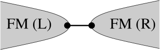
Figure 1: Schematic display of nanoscale magnetic tunnel junction

In this paper we propose theoretically another possible mechanism for the inverse TMR, based on the simple model study. The model system is schematically displayed in Fig. 1, where the spin polarized electrons of one FM electrode pass through a narrow channel into the second FM electrode. When the transmission probability is small between two FM electrodes, the TMR is normal or positive. On the other hand the sign of TMR can become opposite to the case of weak tunneling when the transmission probability is large close to a unity.

The rest of this paper is organized as follows. In Sec. II, the model Hamiltonian is introduced for the nanoscale magnetic tunnel junctions and the spin-polarized current is formulated using the Keldysh nonequilibrium Green’s function technique. The results of our work are presented in Sec. III and a conclusion is included in Sec. IV. In Appendix, we present the tight-binding Hamiltonian approach to the inverse TMR effect in the nanoscale magnetic tunnel junctions.

II Formalism

The considered model system is the magnetic tunnel junction with a very small junction area (linear dimension is of the order of a few Fermi wavelengths). When the junction area is very large compared to the Fermi wave length scale, the Slonczewski model slonczewski will be relevant. The ferromagnetic (FM) metals, which we conveniently call the left ($p=L$) and right ($p=R$) electrodes, are described by the two conduction bands of majority and minority spins. The relative direction of magnetizations in two electrodes is chosen to be arbitrary. It is convenient to write the spin-polarized conduction band in the diagonal basis or the spin quantization direction is chosen to be the direction of magnetization.

$$H_{p} = \sum_{k\sigma}\epsilon_{pk\sigma}c_{pk\sigma}^{{\dagger}}c_{pk\sigma}.$$ (2)

Here $c_{pk\sigma}^{{\dagger}}$ and $c_{pk\sigma}$ are the creation and annihilation operators, respectively, for electrons of wave number $k$ in the electrode $p=L,R$, with the spin direction $\sigma=\pm$. $\sigma=+(-)$ means the spin is aligned parallel (antiparallel) to the direction of magnetization. $\epsilon_{pk\sigma}$ is the energy dispersion relation for electrons in the ferromagnetic metals.

Since the magnetization directions in the left and right electrodes or the spin quantization axes are different, we must be careful when writing the coupling Hamiltonian between two FM electrodes. The flow of electrons from one FM lead to the other is modeled by the transfer Hamiltonian. transfer_ham1 ; transfer_ham2

$$H_{1} = \sum_{kk^{\prime}}\sum_{\alpha\beta}\left[t_{Lk\alpha,Rk^{\prime}\beta}c_{Lk\alpha}^{{\dagger}}c_{Rk^{\prime}\beta}+H.c.\right].$$ (3)

The spin quantization axis (the positive $z$ axis) in this transfer Hamiltonian is chosen to be the direction of the current flow from left to right. In Eq. (3), the spin indices $\alpha,\beta=\uparrow,\downarrow$. $\alpha=\uparrow(\downarrow)$ means the spin is directed parallel (antiparallel) to the positive $z$ direction. Note that we are completely free to choose any direction as the spin quantization direction for this transfer Hamiltonian. After fixing the positive $z$ axis, we can select the orthogonal $x$ and $y$ axes, perpendicular to the $z$ axis, at our disposal. Once the coordinate system is fixed, the direction of magnetization in each FM electrode can be specified by two angles $(\theta_{p},\phi_{p})$ in the spherical coordinates with $p=L,R$ (left, right electrode). Here $\theta_{p}$ measures the angle between the magnetization direction and our chosen $z$ axis, and $\phi_{p}$ is the azimuthal angle of the magnetization measured from the $x$ axis. $t_{Lk\alpha,Rk^{\prime}\beta}$ in Eq. (3) is the hopping integral from the spin band $\beta$ in the right electrode to the spin band $\alpha$ in the left. At this point we consider the most general form of the hopping integral which allows the spin flips. The first term in Eq. (3) represents the transfer of electrons from the right electrode ($R$) with the spin direction $\beta$ to the left ($L$) lead with the spin direction $\alpha$. This transfer Hamiltonian is relevant when the transfer of electrons from one lead to the other occurs dominantly through a very narrow channel (one transport channel).

It is straightforward to show that the electron annihilation operators in two different bases of Eqs. (2) and (3) are related to each other by the equation

$$\begin{pmatrix}c_{pk+}\cr c_{pk-}\end{pmatrix} = \begin{pmatrix}\cos\frac{\theta_{p}}{2}&e^{-i\phi_{p}}\sin\frac{\theta_{p}}{2}\cr-e^{i\phi_{p}}\sin\frac{\theta_{p}}{2}&\cos\frac{\theta_{p}}{2}\end{pmatrix}\begin{pmatrix}c_{pk\uparrow}\cr c_{pk\downarrow}\end{pmatrix}.$$ (4)

Let us introduce the electron spinors ($\Phi$ and $\Psi$) and the unitary transformation matrix ($U$).

$$\Phi_{pk} \equiv \begin{pmatrix}c_{pk+}\cr c_{pk-}\end{pmatrix},~{}~{}~{}\Psi_{pk}~{}\equiv~{}\begin{pmatrix}c_{pk\uparrow}\cr c_{pk\downarrow}\end{pmatrix},$$ (5a)

$$U_{p} \equiv \begin{pmatrix}\cos\frac{\theta_{p}}{2}&-e^{-i\phi_{p}}\sin\frac{\theta_{p}}{2}\cr e^{i\phi_{p}}\sin\frac{\theta_{p}}{2}&\cos\frac{\theta_{p}}{2}\end{pmatrix}.$$ (5b)

The electrode Hamiltonian, Eq (2), is diagonal in the $\Phi$ basis, but not diagonal in the $\Psi$ basis. The two bases are related by the equation, $\Psi_{pk}=U_{p}\Phi_{pk}$, which is none other than Eq. (4). Using the spinor operators, the model Hamiltonian can be written as

$$H_{p} = \sum_{k}\Phi_{pk}^{{\dagger}}\begin{pmatrix}\epsilon_{pk+}&0\cr 0&\epsilon_{pk-}\end{pmatrix}\Phi_{pk},$$ (6a)

$$H_{1} = \sum_{kk^{\prime}}\left[\Psi_{Lk}^{{\dagger}}V_{Lk,Rk^{\prime}}\Psi_{Rk^{\prime}}+H.c.\right],$$ (6b)

$$V_{Lk,Rk^{\prime}} = \begin{pmatrix}t_{Lk\uparrow,Rk^{\prime}\uparrow}&t_{Lk\uparrow,Rk^{\prime}\downarrow}\cr t_{Lk\downarrow,Rk^{\prime}\uparrow}&t_{Lk\downarrow,Rk^{\prime}\downarrow}\end{pmatrix}.$$ (6c)

Here we introduced the hopping matrix $V_{Lk,Rk^{\prime}}$.

We are now in a position to derive the expression of spin-polarized current for our model system. Using the nonequilibrium Green’s function method,neqgreen ; neqgreen1 the electric current flowing from left to right can be computed by thermally averaging the current operator neqgreen2 ; neqgreen3

$$\hat{I} = \frac{e}{i\hbar}\sum_{kk^{\prime}}\sum_{\alpha\beta}\left[t_{Lk\alpha,Rk^{\prime}\beta}c_{Lk\alpha}^{{\dagger}}c_{Rk^{\prime}\beta}-H.c.\right].$$ (7a)

It is now more convenient to write the current operator in the matrix form.

$$\hat{I} = \frac{e}{i\hbar}\sum_{kk^{\prime}}\left[\Psi_{Lk}^{{\dagger}}V_{Lk,Rk^{\prime}}\Psi_{Rk^{\prime}}-\Psi_{Rk^{\prime}}^{{\dagger}}V_{Rk^{\prime},Lk}\Psi_{Lk}\right].$$ (7b)

Let us now introduce the time-ordered mixed Green’s functionsneqgreen ; neqgreen1 which are defined by

$$i\hbar G_{LR}(kt,k^{\prime}t^{\prime}) = \langle T\Psi_{Lk}(t)\Psi_{Rk^{\prime}}^{{\dagger}}(t^{\prime})\rangle,$$ (8a)

$$i\hbar G_{RL}(kt,k^{\prime}t^{\prime}) = \langle T\Psi_{Rk}(t)\Psi_{Lk^{\prime}}^{{\dagger}}(t^{\prime})\rangle,$$ (8b)

where the symbol $\langle A\rangle$ means the thermal average of $A$ and $T$ inside the thermal average means the time-ordering in the Keldysh contour. In terms of the above mixed Green’s functions, the current can be written as

$$I = 2e\sum_{kk^{\prime}}\mbox{Im}\mbox{Tr}\left[V_{Lk,Rk^{\prime}}G_{RL}^{<}(k^{\prime}t,kt)\right]$$ (9)

$$= \frac{2e}{h}\int d\epsilon\sum_{kk^{\prime}}\mbox{Im}\mbox{Tr}\left[V_{Lk,Rk^{\prime}}G_{RL}^{<}(k^{\prime},k;\epsilon)\right].$$

The second line is obtained from the first line after the Fourier transform from time to energy variables.

Since we are mainly interested in the linear response conductance of the system, the physical properties are determined by the energy structure near the Fermi level at low temperature compared with the Fermi temperature. This is the case we are going to consider below. Since the transport properties are mainly determined by electrons near the Fermi level, the dependence of the hopping integral on the wave vector may be neglected and the hopping integral can be replaced by its value at the Fermi energy. From now on, the dependence of the hopping matrix $V_{LR}$ on the wave vector will be suppressed under this approximation scheme. In the tight-binding Hamiltonian approach, the hopping matrix $V_{LR}$ does not depend on the wave vector (see the Appendix for details.) Under this approximation, it is convenient to introduce the wave-vector-summed Green’s functions neqgreen3 to simplify the algebra.

$$G_{p}(t,t^{\prime}) = \sum_{k}G_{p}(k;t,t^{\prime}),~{}~{}~{}p=L,R,$$ (10a)

$$i\hbar G_{p}(k;t,t^{\prime}) \equiv \langle T\Psi_{pk}(t)\Psi_{pk}^{{\dagger}}(t^{\prime})\rangle,$$ (10b)

$$G_{RL}(t,t^{\prime}) = \sum_{kk^{\prime}}G_{RL}(kt;k^{\prime}t^{\prime}).$$ (10c)

Note that $G_{p}(k;t,t^{\prime})$ is the Green’s function of electrons in each lead $p=L,R$ when the coupling between two FM electrodes is absent, while $G_{RL}(kt;k^{\prime}t^{\prime})$ is defined in Eq. (8b). Using the Feynman diagrams, we can readily show that the mixed Green’s function is determined by the Dyson-like equation neqgreen3

$$G_{RL}(t,t^{\prime}) = G_{RL0}(t,t^{\prime})+\int_{C}dt_{1}G_{RL0}(t,t_{1})V_{LR}G_{RL}(t_{1},t^{\prime}),$$ (11)

where the auxiliary Green’s function $G_{LR0}$ is defined as $G_{RL0}(t,t^{\prime})=\int_{C}dt_{1}G_{R}(t,t_{1})V_{RL}G_{L}(t_{1},t^{\prime})$. Here $C$ in the integral sign is the Keldysh contour embracing the real time axis. The Green’s functions $G_{L/R}$ in the above equations can be interpreted as the Green’s function of an electron located at the local tip site of the left/right lead in the absence of the coupling between two FM leads (see the Appendix.) After analytically continuing langreth to the real time axis from the Keldysh contour, it is straightforward to find the lesser Green’s function $G_{RL}^{<}$

$$G_{RL}^{<}(\epsilon) = \left[1-G_{RL0}^{r}(\epsilon)V_{LR}\right]^{-1}G_{RL0}^{<}(\epsilon)\left[1-V_{LR}G_{RL0}^{a}(\epsilon)\right]^{-1},$$ (12)

where the axillary Green’s functions are

$$G_{RL0}^{r,a}(\epsilon) = G_{R}^{r,a}(\epsilon)V_{RL}G_{L}^{r,a}(\epsilon),$$ (13a)

$$G_{RL0}^{<}(\epsilon) = G_{R}^{<}(\epsilon)V_{RL}G_{L}^{a}(\epsilon)+G_{R}^{r}(\epsilon)V_{RL}G_{L}^{<}(\epsilon).$$ (13b)

The $G^{<,r,a}$ denote the lesser, retarded, and advanced Green’s functions, respectively.

To find the expression of the spin-polarized current, we need the explicit forms of the lesser, retarded, and advanced Green’s functions for electrons in the FM electrode. We have to note that the Green’s functions of the FM electrodes in the above equations are not diagonal, because we worked in the spin basis of the transfer Hamiltonian.

$$i\hbar G_{p}(k;t,t^{\prime}) = \langle T\Psi_{pk}(t)\Psi_{pk}^{{\dagger}}(t^{\prime})\rangle~{}=~{}U_{p}\langle T\Phi_{pk}(t)\Phi_{pk}^{{\dagger}}(t^{\prime})\rangle U_{p}^{{\dagger}},$$ (14a)

$$i\hbar g_{p}(k;t,t^{\prime}) = \langle T\Phi_{pk}(t)\Phi_{pk}^{{\dagger}}(t^{\prime})\rangle~{}=~{}\begin{pmatrix}\langle Tc_{pk+}(t)c_{pk+}^{{\dagger}}(t^{\prime})\rangle&0\cr 0&\langle Tc_{pk-}(t)c_{pk-}^{{\dagger}}(t^{\prime})\rangle\end{pmatrix}.$$ (14b)

Here $g_{p}$ is the Green’s functions of the FM electrodes in the spin diagonal basis and related to $G_{p}$ by the unitary transformation, $G_{p}=U_{p}g_{p}U_{p}^{{\dagger}}$. Using the above relations, the desired Green’s functions can be found for the model Hamiltonian of Eq. (2)

$$G_{p}^{r,a}(\epsilon) = U_{p}\sum_{k}\begin{pmatrix}[\epsilon-\epsilon_{pk+}\pm i\delta]^{-1}&0\cr 0&[\epsilon-\epsilon_{pk-}\pm i\delta]^{-1}\end{pmatrix}U_{p}^{{\dagger}},$$ (15a)

$$G_{p}^{<}(\epsilon) = 2\pi f_{p}(\epsilon)U_{p}\sum_{k}\begin{pmatrix}\delta(\epsilon-\epsilon_{pk+})&0\cr 0&\delta(\epsilon-\epsilon_{pk-})\end{pmatrix}U_{p}^{{\dagger}}.$$ (15b)

Here an infinitesimally small positive number $\delta$ is included for the definition of the retarded ($+$ sign) and advanced ($-$ sign) Green’s functions, $G_{p}^{r,a}$. $f_{p}(\epsilon)=f(\epsilon-\mu_{p})$ is the Fermi-Dirac thermal distribution function in the lead $p=L,R$ and $\mu_{p}$ is the chemical potential shift of each lead caused by the source-drain bias voltage. Let us define $R_{p\pm}$ and $N_{p\pm}$ as

$$R_{p\pm}(\epsilon) = {\cal P}\sum_{k}\frac{1}{\epsilon-\epsilon_{pk\pm}},$$ (16a)

$$N_{p\pm}(\epsilon) = \sum_{k}\delta(\epsilon-\epsilon_{pk\pm}),$$ (16b)

where ${\cal P}$ means the principal part of the integral. $N_{p\pm}(\epsilon)$ is none other than the density of states (DOS) for the majority/minority spin in the FM lead $p=L,R$. The retarded, advanced, and lesser Green’s functions [Eqs. (15a) and (15b)] can be written as

$$G_{p}^{r,a}(\epsilon) = U_{p}[R_{p}\mp i\pi N_{p}]U_{p}^{{\dagger}},$$ (17a)

$$G_{p}^{<}(\epsilon) = 2\pi f_{p}(\epsilon)U_{p}N_{p}U_{p}^{{\dagger}},$$ (17b)

where $R_{p}=\left(\begin{smallmatrix}R_{p+}&0\cr 0&R_{p-}\end{smallmatrix}\right)$ and $N_{p}=\left(\begin{smallmatrix}N_{p+}&0\cr 0&N_{p-}\end{smallmatrix}\right)$. When the Fermi level lies inside the band, $R_{p\pm}(\epsilon=E_{F})$ is expected to be small due to the mutual cancellation of electron (above the Fermi level) and hole (below the Fermi level) contributions. In this case or in a wide conduction band limit,wideband we can set $R_{p\pm}(\epsilon=E_{F})\approx 0$. The retarded and advanced Green’s functions are given in simple forms in this case.

$$G_{p}^{r,a}(\epsilon) = \mp i\pi U_{p}N_{p}U_{p}^{{\dagger}}.$$ (18)

For half metals with only one spin band occupied at the Fermi level, the value of $R$ for unoccupied spin band may not be neglected such that the retarded and advanced Green’s functions may have real component.

When the Fermi level lies well inside the band for both spin directions or in a wide band limit,wideband we can approximately set $R_{p\pm}\approx 0$. In this case, inserting the Eqs. (17b) and (18) into Eqs. (13), the expressions of $G_{RL0}^{r,a}$ and $G_{RL0}^{<}$ can be simplified as

$$G_{RL0}^{r,a}(\epsilon) = -\pi^{2}\hat{N}_{R}V_{RL}\hat{N}_{L},$$ (19a)

$$G_{RL0}^{<}(\epsilon) = 2i\pi^{2}\left[f_{R}(\epsilon)-f_{L}(\epsilon)\right]\hat{N}_{R}V_{RL}\hat{N}_{L},$$ (19b)

where $\hat{N}_{p}=U_{p}N_{p}U_{p}^{{\dagger}}$. Inserting these two Eqs. (19) into Eq. (12), we find for the lesser Green’s function $G_{RL}^{<}$

$$G_{RL}^{<} = 2i\pi^{2}\left[f_{R}(\epsilon)-f_{L}(\epsilon)\right]\left[1+\pi^{2}\hat{N}_{R}V_{RL}\hat{N}_{L}V_{LR}\right]^{-1}$$ (20)

$$\times\hat{N}_{R}V_{RL}\hat{N}_{L}\left[1+\pi^{2}V_{LR}\hat{N}_{R}V_{RL}\hat{N}_{L}\right]^{-1}.$$

Combining this lesser Green’s function and Eq. (9), the expression of the spin-polarized current can be written as

$$I = \frac{2e}{h}\int d\epsilon\mbox{Im}\mbox{Tr}\left[V_{LR}G_{RL}^{<}(\epsilon)\right]$$ (21)

$$= \frac{2e}{h}\int d\epsilon\left[f_{R}(\epsilon)-f_{L}(\epsilon)\right]T(\epsilon),$$

where

$$T(\epsilon) = 2\mbox{Re}\mbox{Tr}[1+\Gamma]^{-1}\Gamma[1+\Gamma]^{-1},$$ (22a)

$$\Gamma = \pi^{2}\hat{N}_{R}V_{RL}\hat{N}_{L}V_{LR}.$$ (22b)

In obtaining the above form of $T(\epsilon)$, the trace property of the matrix product was invoked. Here $T(\epsilon)$ is the transmission probability through a narrow channel for spin-polarized electrons, when the magnetization directions of two FM electrodes are arbitrary. The information about the orientation of two magnetizations is included in the DOS matrices, $\hat{N}_{L}$ and $\hat{N}_{R}$. The matrix $\Gamma$ measures the effective transfer rate of spin-polarized electrons from one FM electrode to the other FM electrode, and contains the dependence on the relative orientation of two magnetizations. The above form of the transmission probability is valid for the wide band case or when the Fermi level lies well inside the bands for both spin directions. The linear response conductance $G$ is then given by the expression, $G=\frac{2e^{2}}{h}\cdot T(\epsilon=0)$. Below we are going to confine our interest to the linear response regime and to the case of a wide band limit.

We can give some physical meaning to the density matrix $\hat{N}_{p}=U_{p}N_{p}U_{p}^{{\dagger}}$. After some algebra, $\hat{N}_{p}$ can be expressed as

$$\hat{N}_{p} = N_{p0}[1+P_{p}\hat{n}_{p}\cdot\vec{\sigma}],$$ (23a)

$$N_{p0} = =\frac{1}{2}[N_{p+}+N_{p-}],$$ (23b)

$$P_{p} = \frac{N_{p+}-N_{p-}}{N_{p+}+N_{p-}}.$$ (23c)

Here $\vec{\sigma}$ is the Pauli matrices, $N_{p0}$ is the average DOS of the majority and minority spin bands. $P_{p}$ measures the spin polarization at a given energy $\epsilon$ of the FM electrode $p=L,R$ and agrees with the definition of the spin polarization in the Julliere model. julliere $\hat{n}_{p}$ is the unit vector defined by the two angles, $\theta_{p}$ and $\phi_{p}$ in the spherical coordinate system and is aligned parallel to the magnetization direction of the $p=L,R$ FM electrode.

III Results and discussion

In this section we study the TMR behavior for the wide band case with the transfer Hamiltonian: $t_{L\alpha,R\beta}=t_{LR}\delta_{\alpha\beta}$. Electrons do not flip their spin while passing through the narrow channel. In this case the expression of $\Gamma$ in the transmission probability, Eq. (22a), is simplified as

$$\Gamma = \pi^{2}|t_{LR}|^{2}\hat{N}_{R}\hat{N}_{L}$$ (24)

$$= \gamma(1+P_{R}\hat{n}_{R}\cdot\vec{\sigma})(1+P_{L}\hat{n}_{L}\cdot\vec{\sigma}).$$

Here $\gamma\equiv\pi^{2}N_{L0}N_{R0}|t_{LR}|^{2}$ measures the average transfer rate of electrons for two spin directions. The expression of the transmission probability $T$ is

$$T(\epsilon) = 4\gamma\times\frac{1+\vec{P}_{L}\cdot\vec{P}_{R}+\gamma(1-P_{L}^{2})(1-P_{R}^{2})(2+\gamma+\gamma\vec{P}_{L}\cdot\vec{P}_{R})}{[1+2\gamma(1+\vec{P}_{L}\cdot\vec{P}_{R})+\gamma^{2}(1-P_{L}^{2})(1-P_{R}^{2})]^{2}}.$$ (25)

Note that $\vec{P}_{L}=\hat{n}_{L}P_{L}$ and $\vec{P}_{R}=\hat{n}_{R}P_{R}$. This is the most general result for the magnetic tunnel junctions with a narrow junction area. Note that the conductance, $2e^{2}/h\times T(0)$, depends only on the relative angle of two magnetization directions. In the weak tunneling limit or $\gamma\ll 1$, the transmission probability can be approximated as $T=4\gamma(1+\vec{P}_{L}\cdot\vec{P}_{R})=4\gamma(1+P_{L}P_{R}\cos\theta)$. The conductance is then given by the expression, $G=G_{0}(1+P_{L}P_{R}\cos\theta)$ with $G_{0}=8\gamma e^{2}/h$. This is the familiar expression of the conductance which is in agreement with the Julliere model.julliere The TMR ratio is then $TMR=2P_{L}P_{R}/(1-P_{L}P_{R})$. In the weak tunneling limit, the TMR is determined solely by the polarization of the ferromagnetic metals. In the strong tunneling limit the angle dependence of the conductance is still an even function of $\theta$, but is more complicated as shown in Eq. (25).

When two ferromagnetic electrodes are the same ($N_{L+}=N_{R+}=N_{+}$ and $N_{L-}=N_{R-}=N_{-}$) with the possible difference in the magnetization direction, we have $P_{L}=P_{R}=P$. The expression of $T$, Eq. (25), is further simplified

$$T(\cos\theta) = 4\times\frac{\gamma(1+P^{2}\cos\theta)+\gamma^{2}(1-P^{2})^{2}(2+\gamma[1+P^{2}\cos\theta])}{\left[1+2\gamma(1+P^{2}\cos\theta)+\gamma^{2}(1-P^{2})^{2}\right]^{2}}.$$ (26)

Especially for the parallel ($\cos\theta=1$) and antiparallel ($\cos\theta=-1$) configurations, the transmission probabilities, respectively, given by the expressions

$$T_{P} = \frac{2\gamma_{+}}{(1+\gamma_{+})^{2}}+\frac{2\gamma_{-}}{(1+\gamma_{-})^{2}},$$ (27a)

$$T_{AP} = \frac{4\sqrt{\gamma_{+}\gamma_{-}}}{(1+\sqrt{\gamma_{+}\gamma_{-}})^{2}}.$$ (27b)

Here $\gamma_{\pm}$ is defined by the equation $\gamma_{\pm}\equiv\pi^{2}N_{\pm}^{2}|t_{LR}|^{2}$ ($0<\gamma_{\pm}\leq 1$), and is related to the transmission probability $T_{\pm}$ by the relation

$$T_{\pm} = \frac{4\gamma_{\pm}}{(1+\gamma_{\pm})^{2}}.$$ (28)

$T_{+}$ is the transmission probability for electrons from the majority band in the left electrode to the majority band in the right electrode, while $T_{-}$ from minority to minority. Note that the average transfer rate $\gamma$ and the polarization $P$ are related to the transfer rates of majority and minority spins by the equations

$$\gamma = \frac{1}{4}[\sqrt{\gamma_{+}}+\sqrt{\gamma_{-}}]^{2},$$ (29a)

$$P = \frac{\sqrt{\gamma_{+}}-\sqrt{\gamma_{-}}}{\sqrt{\gamma_{+}}+\sqrt{\gamma_{-}}}.$$ (29b)

The transmission probabilities, $T_{P}$ and $T_{AP}$, can be expressed in terms of $T_{\pm}$ as $T_{P}=\frac{1}{2}(T_{+}+T_{-})$ and $T_{AP}=4\sqrt{T_{+}T_{-}}(1+\sqrt{1-T_{+}})(1+\sqrt{1-T_{-}})[\sqrt{T_{+}T_{-}}+(1+\sqrt{1-T_{+}})(1+\sqrt{1-T_{-}})]^{-2}$.

In the weak tunneling limit $T_{\pm}\ll 1$ or $\gamma_{\pm}\ll 1$, the Eq. (26) can be approximated as $T(\cos\theta)=4\gamma(1+P^{2}\cos\theta)$. Especially for the parallel and antiparallel configurations, we have $T_{P}=2(\gamma_{+}+\gamma_{-})$ and $T_{AP}=4\sqrt{\gamma_{+}\gamma_{-}}$. Since $\gamma_{+}+\gamma_{-}\geq 2\sqrt{\gamma_{+}\gamma_{-}}$, we have the conductance inequality $G_{P}\geq G_{AP}$. This inequality relation is true generally when the transmission probability is weak. That is, the current flows more in the parallel configuration than in the antiparallel configuration.

Figure 2: Inverse TMR. (a) Dependence of TMR on the transmission probabilities of electrons for majority ($T_{+}$) and minority spin ($T_{-}$). The dashed line is the boundary between the positive and negative TMR. (b) Sign of TMR in parameter space of $(T_{+},T_{-})$. TMR vanishes along the solid and dashed lines. Two lines meet at $T_{+}=T_{-}=2/3$. The TMR becomes negative when the tunneling probabilities for electrons of both spin directions is close to a unity. The curve $T_{+}=T_{-}$ (solid line) corresponds to the nonmagnetic electrodes.

In the strong tunneling limit, the above inequality in conductance can be reversed and more current can flow in the antiparallel alignment than in the parallel alignment. To see when the current flows more in the AP than in the P, we study $T_{P}$ and $T_{AP}$ [Eqs. (27a) and (27b)] in the plane of $(\gamma_{+},\gamma_{-})$ or $(T_{+},T_{-})$. The curves on which $T_{P}=T_{AP}$ are given by the equations

$$0 = \gamma_{+}-\gamma_{-},$$ (30a)

$$0 = (\gamma_{+}\gamma_{-}-1)^{2}-2\sqrt{\gamma_{+}\gamma_{-}}(1+\gamma_{+})(1+\gamma_{-}).$$ (30b)

Along these two curves the conductance in the P and AP configurations is equal. The curve $\gamma_{+}=\gamma_{-}$ corresponds to the case that $T_{P}=T_{AP}$ and the magnetic polarization at the Fermi energy is zero or $P=0$. The second curve, Eq. (30b), is the boundary between two regions: $T_{P}>T_{AP}$ (close to the origin) and $T_{P}<T_{AP}$ (strong tunneling regime), and corresponds to the case that $P\neq 0$, but $T_{P}=T_{AP}$. Two curves meet each other at $(\gamma_{+},\gamma_{-})=(2-\sqrt{3},2-\sqrt{3})$, which corresponds to the point $(T_{+},T_{-})=(2/3,2/3)$ in the plane of transmission probabilities. The behavior of TMR is summarized in Fig. 2(a) and (b). The value of TMR is plotted as a function of $(T_{+},T_{-})$ in the panel (a) and the boundary between normal and inverse TMR is marked by the dashed line. The panel (b) provides the TMR diagram in the $(T_{+},T_{-})$ plane. Especially in the strong tunneling limit, the inverse TMR can be realized in the nanoscale magnetic tunnel junctions.

Figure 3: Dependence of conductance on the relative angle between two magnetization directions with varying transmission probability $T_{+}$ for the majority spin. In panel (a) $P=33\%$ is chosen to simulate the Ni electrodes,review while $P=55\%$ in panel (b) for CoFe electrodes. The solid line ($T_{+}<<1$) corresponds to the Julliere result or the very weak tunneling limit.

Fig. 3 displays the conductance ratio, $G(\theta)/G_{P}$, as a function of the relative angle between two directions of magnetization [$G_{P}=G(\theta=0)]$. While the polarization is fixed, the transmission probabilities are varied. In the weak tunneling limit the solid curve traces the cosine function. With increasing transmission probabilities, the curves deviate from the Julliere result and furthermore the conductance minimum can change into a maximum leading to the inverse TMR.

IV Summary and conclusion

To summarize, we studied the spin-polarized transport through a narrow channel using the transfer Hamiltonian approach and the nonequilibrium Green’s function method. Our analysis applies to the case when the Fermi level lies well inside both majority and minority spin bands or to the wide band limit. In the weak tunneling limit we reproduce the Julliere results and the TMR is positive. On the other hand, in the strong tunneling limit the inverse TMR opposite to the weak tunneling case is found. We presented another theoretical scenario for the inverse TMR effect. Our model study may be relevant to the magnetic junctions with a quantum point contact between two ferromagnetic metals or to the thick planar MTJs with a pinhole which accommodate only one transport channel.

Appendix A Tight-binding model for the ferromagnetic electrodes

To illustrate the relevance of our approach to real systems, we consider the description of the ferromagnetic (FM) electrodes in terms of the tight-binding Hamiltonian. Two FM electrodes are coupled by the hopping term between two atomic sites. Though our formalism can be generally applied to any types of lattice, we confine our study to the lattices for which the analytic solution of the Green’s functions can be readily found. The examples include the Bethe lattice out of which the simplest one is the semi-infinite one-dimensional tight-binding atomic chain (see Fig. 4.)

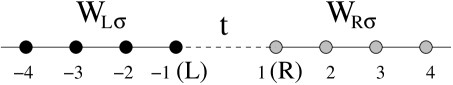
Figure 4: Tight-binding model for the FM electrodes. The FM electrodes are described by the semi-infinite chain. The site of $i=-1(i=1)$ is the terminal site of the left (right) electrode, and is denoted as $i=L(i=R)$ for the notational convenience.

The left and right electrodes are described by the tight-binding Hamiltonian

$$H_{L} = \sum_{i\leq-1}\sum_{\sigma=\pm}\epsilon_{L\sigma}c_{i\sigma}^{{\dagger}}c_{i\sigma}-\sum_{i\leq-2}\sum_{\sigma=\pm}\left[W_{L\sigma}c_{i+1\sigma}^{{\dagger}}c_{i\sigma}+H.c.\right],$$ (31a)

$$H_{R} = \sum_{i\geq 1}\sum_{\sigma=\pm}\epsilon_{R\sigma}c_{i\sigma}^{{\dagger}}c_{i\sigma}-\sum_{i\geq 1}\sum_{\sigma=\pm}\left[W_{R\sigma}c_{i+1\sigma}^{{\dagger}}c_{i\sigma}+H.c.\right].$$ (31b)

The left (right) FM electrode is terminated at the site of $i=-1$ or $i=L$ ($i=1$ or $i=R$), respectively. The $i=L$ site will be called the left terminal site and the $i=R$ site the right terminal site. The electron creation ($c_{i\sigma}^{{\dagger}}$) and annihilation ($c_{i\sigma}$) operators are defined in the spin diagonal basis. $\sigma=+(-)$ means the spin is aligned parallel (antiparallel) to the magnetization, respectively. However the spin quantization directions of two leads are different due to different magnetization directions. The on-site energies, $\epsilon_{L\sigma}$ and $\epsilon_{R\sigma}$, include the exchange splitting between two spin directions as well as a possible voltage difference between two FM leads. In order to take into account the different bandwidth of spin-up and spin-down bands, the hopping integrals, spinband $W_{L\sigma}$ and $W_{R\sigma}$, include the spin index $\sigma=\pm$. Magnetic polarization is determined by the values of on-site energies and hopping integrals.

Adopting the same convention for the direction of spin quantization (chosen to be the direction of the current flow from left to right) as in the main text, the hopping term which is responsible for the flow of electrons between two leads can be written as

$$H_{1} = \sum_{\alpha\beta}\left[t_{L\alpha,R\beta}c_{L\alpha}^{{\dagger}}c_{R\beta}+H.c.\right].$$ (32)

Here $\alpha,\beta=\uparrow,\downarrow$ and the $\uparrow(\downarrow)$ direction is parallel (antiparallel) to the spin quantization direction. Since the spin quantization directions in Eqs. (31) and Eq. (32) are different, the electron operators in two spin bases are related to each other by the unitary transformation. For details, see the main text.

$$\Phi_{p} \equiv \begin{pmatrix}c_{p+}\cr c_{p-}\end{pmatrix},~{}~{}~{}\Psi_{p}~{}\equiv~{}\begin{pmatrix}c_{p\uparrow}\cr c_{p\downarrow}\end{pmatrix},$$ (33a)

$$U_{p} \equiv \begin{pmatrix}\cos\frac{\theta_{p}}{2}&-e^{-i\phi_{p}}\sin\frac{\theta_{p}}{2}\cr e^{i\phi_{p}}\sin\frac{\theta_{p}}{2}&\cos\frac{\theta_{p}}{2}\end{pmatrix}.$$ (33b)

The two bases are related by the equation, $\Psi_{p}=U_{p}\Phi_{p}$ for $p=L,R$. Obviously the two bases at other sites are related to each other by the same unitary transformation. Using the nonequilibrium Green’s function method, the spin-polarized current can be expressed as

$$I = \frac{2e}{h}\int d\epsilon~{}\mbox{Im}\mbox{Tr}V_{LR}G_{RL}^{<}(\epsilon),$$ (34)

where the hopping matrix $V_{LR}$ and the Green’s function are defined as

$$V_{LR} = \begin{pmatrix}t_{L\uparrow,R\uparrow}&t_{L\uparrow,R\downarrow}\cr t_{L\downarrow,R\uparrow}&t_{L\downarrow,R\downarrow}\end{pmatrix},$$ (35)

$$i\hbar G_{RL}(t,t^{\prime}) = \langle T\Psi_{R}(t)\Psi_{L}^{{\dagger}}(t^{\prime})\rangle.$$ (36)

Note that the hopping matrix has no dependence on the wave vector in the tight-binding Hamiltonian approach. Here $G_{RL}(t,t^{\prime})$ is the time-ordered Green’s function and $G_{RL}^{<}$ is the lesser part of $G_{RL}$. After Fourier transform over time variable, the lesser Green’s function $G_{RL}^{<}$ can be found in a closed form (see the main text and also [neqgreen2, ].)

$$G_{RL}^{<}(\epsilon) = \left[1-G_{RL0}^{r}(\epsilon)V_{LR}\right]^{-1}G_{RL0}^{<}(\epsilon)$$ (37)

$$\times\left[1-V_{LR}G_{RL0}^{a}(\epsilon)\right]^{-1},$$

$$G_{RL0}^{r,a}(\epsilon) = G_{R}^{r,a}(\epsilon)V_{RL}G_{L}^{r,a}(\epsilon),$$ (38)

$$G_{RL0}^{<}(\epsilon) = G_{R}^{<}(\epsilon)V_{RL}G_{L}^{a}(\epsilon)+G_{R}^{r}(\epsilon)V_{RL}G_{L}^{<}(\epsilon).$$ (39)

Here $G_{L}$ and $G_{R}$ are the Green’s functions at the left and right terminal sites, respectively, when the coupling between two FM electrodes is absent.

$$i\hbar G_{p}(t,t^{\prime}) = \langle T\Psi_{p}(t)\Psi_{p}^{{\dagger}}(t^{\prime})\rangle~{}=~{}U_{p}\langle T\Phi_{p}(t)\Phi_{p}^{{\dagger}}(t^{\prime})\rangle U_{p}^{{\dagger}},~{}~{}~{}p=L,R.$$ (40)

The superscripts $r,a$ and $<$ mean the retarded, advanced, and lesser part of the Green’s function. To compute the spin-polarized current, we have only to find the Green’s functions at the terminal site ($L$ or $R$) when the coupling between two FM electrodes is absent. It is convenient to define the terminal Green’s function in the spin diagonal basis

$$i\hbar g_{p}(t,t^{\prime}) = \langle T\Phi_{p}(t)\Phi_{p}^{{\dagger}}(t^{\prime})\rangle~{}=~{}\begin{pmatrix}\langle Tc_{p+}(t)c_{p+}^{{\dagger}}(t^{\prime})\rangle&0\cr 0&\langle Tc_{p-}(t)c_{p-}^{{\dagger}}(t^{\prime})\rangle\end{pmatrix}.$$ (41)

This Green’s function $g_{p}=\left(\begin{smallmatrix}g_{p+}&0\cr 0&g_{p-}\end{smallmatrix}\right)$ is diagonal and is related to $G_{p}$ by the unitary transformation, $G_{p}=U_{p}g_{p}U_{p}^{{\dagger}}$.

At this point we had better take a concrete example for the terminal Green’s functions, $g_{L}$ and $g_{R}$ (in the spin diagonal basis). As an example we consider the semi-infinite chain model for the FM electrodes. It is relatively simple to find the self-energy of the terminal Green’s function, when we take into account the repeating structure of the chain. The self-energy can be expressed in terms of the Green’s function itself ($p=L,R$).

$$\Sigma_{p}(t,t^{\prime}) = \begin{pmatrix}|W_{p+}|^{2}g_{p+}(t,t^{\prime})&0\cr 0&|W_{p-}|^{2}g_{p-}(t,t^{\prime})\end{pmatrix}.$$ (42)

From the Dyson equation, we can find the desired Green’s functions in a straightforward manner. The retarded and advanced Green’s functions are

$$g_{p\sigma}^{r,a}(\epsilon) = \frac{2}{\epsilon-\epsilon_{p\sigma}\pm i\sqrt{4|W_{p\sigma}|^{2}-(\epsilon-\epsilon_{p\sigma})^{2}}}.$$ (43)

The retarded part ($r$) corresponds to the $+$ sign, while the advanced part ($a$) to the $-$ sign. Quite in general, the retarded and advanced Green’s functions at the terminal site can be written in a form $g_{p\sigma}^{r}(\epsilon)=R_{p\sigma}(\epsilon)-i\pi N_{p\sigma}(\epsilon)$ and $g_{p\sigma}^{a}=[g_{p\sigma}^{r}]^{*}$, respectively, such that we can write the matrix Green’s function as

$$g_{p}^{r,a}(\epsilon) = \begin{pmatrix}R_{p+}(\epsilon)&0\cr 0&R_{p-}(\epsilon)\end{pmatrix}\mp i\pi\begin{pmatrix}N_{p+}(\epsilon)&0\cr 0&N_{p-}(\epsilon)\end{pmatrix}~{}=~{}R_{p}(\epsilon)\mp i\pi N_{p}(\epsilon).$$ (44)

Here $N_{p\sigma}$ is the local density of states (DOS) or the local spectral function at the terminal site in the spin state $\sigma=\pm$. The lesser Green’s function at the terminal site is simply related to the DOS matrix $N_{p}=\left(\begin{smallmatrix}N_{p+}&0\cr 0&N_{p-}\end{smallmatrix}\right)$ by the expression, $g_{p}^{<}=2\pi f_{p}(\epsilon)N_{p}$.

Once the terminal Green’s functions are known in the diagonal basis, the algebra becomes straightforward to reduce the expression of the spin-polarized current, Eq. (34). Then the desired Green’s functions at the terminal sites are ($p=L,R$)

$$G_{p}^{r,a}(\epsilon) = U_{p}\begin{pmatrix}g_{p+}^{r,a}(\epsilon)&0\cr 0&g_{p-}^{r,a}(\epsilon)\end{pmatrix}U_{p}^{{\dagger}},$$ (45)

$$G_{p}^{<}(\epsilon) = 2\pi f_{p}(\epsilon)U_{p}N_{p}U_{p}^{{\dagger}}.$$ (46)

To simplify the notations we rewrite

$$G_{p}^{r,a}(\epsilon) = \hat{R}_{p}\mp i\pi\hat{N}_{p},$$ (47)

$$G_{p}^{<}(\epsilon) = 2\pi f_{p}(\epsilon)\hat{N}_{p},$$ (48)

where $\hat{N}_{p}=U_{p}N_{p}U_{p}^{{\dagger}}$ and $\hat{R}_{p}=U_{p}R_{p}U_{p}^{{\dagger}}$. The expression of $G_{RL0}^{<}$ can be rearranged as

$$G_{RL0}^{<} = 2i\pi^{2}[f_{R}-f_{L}]\hat{N}_{R}T_{RL}\hat{N}_{L}$$ (49)

$$+2\pi\left[f_{R}\hat{N}_{R}T_{RL}\hat{R}_{L}+f_{L}\hat{R}_{R}T_{RL}\hat{N}_{L}\right].$$

From now on we consider the case of no spin-flip in tunneling of electrons between two FM electrodes or $T_{RL}=t_{RL}{\bf 1}$. We also confine our interest to the case that two FM electrodes are the same material. Then we can derive the simpler relation for the spin-polarized current.

$$G_{RL0}^{<} = 2it_{RL}\pi^{2}[f_{R}-f_{L}]\hat{N}_{R}\hat{N}_{L}$$ (50)

$$+2\pi t_{RL}\left[f_{R}\hat{N}_{R}\hat{R}_{L}+f_{L}\hat{R}_{R}\hat{N}_{L}\right],$$

$$\mbox{Tr}\{T_{RL}G_{RL}^{<}\} = t_{LR}\mbox{Tr}\left\{[1-t_{LR}G_{RL0}^{r}]^{-1}G_{RL0}^{<}\right.$$ (51)

$$\times\left.[1-t_{LR}G_{RL0}^{a})]^{-1}\right\}.$$

From these two relations, we find the simple expression for $\mbox{Im}\mbox{Tr}T_{LR}G_{RL}^{<}$ in the parallel and antiparallel alignments of magnetizations such that the expression of the spin-polarized current is

$$I = \frac{2e}{h}\int d\epsilon~{}[f_{R}(\epsilon)-f_{L}(\epsilon)]~{}T(\epsilon),$$ (52)

$$T(\epsilon) = 2\pi^{2}|t_{LR}|^{2}~{}\mbox{Tr}\left\{[1-t_{LR}G_{RL0}^{r}]^{-1}\hat{N}_{R}\hat{N}_{L}\right.$$ (53)

$$\left.[1-t_{LR}G_{RL0}^{a}]^{-1}\right\}.$$

Since we are considering two FM electrodes of the same material, we have for the parallel alignment of magnetizations

$$\hat{N}_{L} = \hat{N}_{R}~{}=~{}\begin{pmatrix}N_{+}&0\cr 0&N_{-}\end{pmatrix},$$ (54)

$$G_{RL0}^{r,a} = t_{RL}\begin{pmatrix}(R_{+}\mp i\pi N_{+})^{2}&0\cr 0&(R_{-}\mp i\pi N_{-})^{2}\end{pmatrix}.$$ (55)

The transmission probability for this case is

$$T_{P}(\epsilon) = \sum_{\sigma=\pm}\frac{2\pi^{2}|t_{LR}|^{2}N_{\sigma}^{2}}{\left|1-[t_{LR}g_{\sigma}]^{2}\right|^{2}},$$ (56)

where $g_{\sigma}=R_{\sigma}+i\pi N_{\sigma}$. For the antiparallel alignment of magnetizations, we have

$$\hat{N}_{L} = \begin{pmatrix}N_{+}&0\cr 0&N_{-}\end{pmatrix},~{}~{}~{}\hat{N}_{R}~{}=~{}\begin{pmatrix}N_{-}&0\cr 0&N_{+}\end{pmatrix},$$ (57)

$$G_{RL0}^{r,a} = t_{RL}(R_{+}\mp i\pi N_{+})(R_{-}\mp i\pi N_{-})~{}{\bf 1},$$ (58)

such that the transmission probability is given by the expression

$$T_{AP}(\epsilon) = \frac{4\pi^{2}|t_{LR}|^{2}N_{+}N_{-}}{\left|1-|t_{LR}|^{2}g_{+}g_{-}\right|^{2}}.$$ (59)

We are now in a position to discuss any possible inverse tunneling magnetoresistance effect for the narrow channel magnetic tunnel junctions.

In a weak tunneling limit or when $|t_{LR}g_{\sigma}^{r}|\ll 1$, the transmission probabilities for the parallel and antiparallel alignments of magnetizations can be approximated as

$$T_{P} = 2\pi^{2}|t_{LR}|^{2}\left[N_{+}^{2}+N_{-}^{2}\right],$$ (60)

$$T_{AP} = 4\pi^{2}|t_{LR}|^{2}N_{+}N_{-}.$$ (61)

Obviously $T_{P}>T_{AP}$ such that more current flows in P than in AP, and the positive TMR ratio is obtained with the familiar Julliere expression.

In a strong tunneling limit, let us see if there is a possibility of $T_{P}<T_{AP}$. To be concrete let us consider the semi-infinite chain model. Note that the Eq. (43) can be written as

$$g_{p\sigma}^{r}(\epsilon) = \frac{1}{|W_{p\sigma}|}\left[\frac{\epsilon-\epsilon_{p\sigma}}{2|W_{p\sigma}|}-i\sqrt{1-\frac{(\epsilon-\epsilon_{p\sigma})^{2}}{4|W_{p\sigma}|^{2}}}\right]$$ (62)

and $g_{p\sigma}^{a}=[g_{p\sigma}^{r}]^{*}$. Since we are interested in the linear response transport, we have only to consider the terminal Green’s functions at the Fermi level or $\epsilon=0$. In a wide band limit or when $|\epsilon_{p\sigma}|\ll|W_{p\sigma}|$, the terminal Green’s functions are reduced to $g_{p\sigma}^{r}\approx-i/|W_{p\sigma}|$ and $g_{p\sigma}^{a}\approx i/|W_{p\sigma}|$ such that our discussion corresponds exactly to our study in the main text. When $R_{\pm}=0$, the transmission probabilities for the tight-binding model are exactly the same as those in the main text. It is expected that the inverse TMR is possible when $|R|\ll N$.

References

• (1) E. Y. Tsymbal, O. N. Mryasov, and P. R. LeClair, J. Phys.: Condens. Matter 15, 109 (2003).
• (2) I. Zutic, J. Fabian, and S. D. Sarma, Rev. Mod. Phys. 76, 323 (2004).
• (3) J. S. Moodera, L. R. Kinder, T. M. Wong, and R. Meservey, Phys. Rev. Lett. 74, 3273 (1995).
• (4) T. Miyazaki and N. J. Tezuka, J. Magn. Magn. Mater. 139, L231 (1995).
• (5) M. Julliere, Phys. Lett. 54A, 225 (1975).
• (6) J. M. De Teresa, A. BarthΓ©lΓ©my, A. Fert, J. P. Contour, R. Lyonnet, F. Montaigne, P. Seneor, and A. VaurΓ¨s, Phys. Rev. Lett. 82, 4288 (1999).
• (7) J. M. De Teresa, A. BarthΓ©lΓ©my, A. Fert, J. P. Contour, F. Montaigne, and P. Seneor, Science 286, 507 (1999).
• (8) M. Sharma, S. X. Wang, and J. H. Nickel, Phys. Rev. Lett. 82, 616 (1999).
• (9) E. Y. Tsymbal, A. Sokolov, I. F. Sabirianov, and B. Doudin, Phys. Rev. Lett. 90, 186602 (2003).
• (10) A. N. Pasupathy, R. C. Bialczak, J. Martinek, J. E. Grose, L. A. K. Donev, P. L. McEuen, and D. C. Ralph, Science 306, 86 (2004).
• (11) E. Y. Tsymbal and D. G. Pettifor, J. Phys.: Condens. Matter 9, L411 (1997).
• (12) K. Wang, S. Zhang, P. M. Levy, L. Szunyogh and P. Weinberger, J. Magn. Mag. Mater. 189, L131 (1998).
• (13) W. H. Butler, X.-G. Zhang, T. C. Schulthess, and J. M. MacLaren, Phys. Rev. B 63, 054416 (2001).
• (14) P. Zhang, Q.-K. Xue, Y. Wang, and X. C. Xie, Phys. Rev. Lett. 89, 286803 (2002); J. Martinek, Y. Utsumi, H. Imamura, J. BarnaΕ›, S. Maekawa, J. KΓΆnig, and G. SchΓΆn, ibid 91, 127203 (2003); M.-S. Choi, D. SΓ‘nchez, and R. LΓ³pez, ibid 92, 056601 (2004).
• (15) J. C. Slonczewski, Phys. Rev. B 39, 6995 (1989).
• (16) J. Bardeen, Phys. Rev. Lett. 6, 57 (1961).
• (17) T. E. Feuchtwang, Phys. Rev. B 10, 4121 (1974); ibid 10, 4135 (1974).
• (18) L. P. Kadanoff and G. Baym, Quantum Statistical Mechanics (Benjamin, New York, 1962).
• (19) L.V. Keldysh, Zh. Γ‰ksp. Teor. Fiz. 47, 1515 (1964). [Sov. Phys. JETP 20, 1018 (1965)].
• (20) T.-S. Kim and S. Hershfield, Phys. Rev. B 63, 245326 (2001).
• (21) T.-S. Kim and S. Hershfield, Phys. Rev. Lett. 88, 136601 (2002); Phys. Rev. B 67, 165313 (2003).
• (22) D.C. Langreth, 1976, in Linear and Nonlinear Electron Transport in Solids, Vol.17 of NATO Advanced Study Institute, Series B: Physicsi, edited by J.T. Devreese and V.E. van Doren (Plenum, New York, 1976), p. 3.
• (23) The meaning of a wide band limit is clarified in the Appendix. See, for example, S. Hershfield, J. H. Davies, and J. W. Wilkins, Phys. Rev. Lett. 67, 3720 (1991).
• (24) See, for example, M. Zwolak and M. Di Ventra, Appl. Phys. Lett. 81, 925 (2002).