Interferometry in dense nonlinear media and interaction-induced loss of contrast in microfabricated atom interferometers

Abstract

In this paper we update the existing schemes for computation of atom-interferometric signal in single-atom interferometers to interferometry with dense Bose-condensed atomic samples. Using the theory developed we explain the fringe contrast degradation observed, for longer duration of interferometric cycle, in the Michelson interferometer on a chip recently realized at JILA (Ying-Ju Wang, Dana Z. Anderson, Victor M. Bright, Eric A. Cornell, Quentin Diot, Tetsuo Kishimoto, Mara Prentiss, R. A. Saravanan, Stephen R. Segal, Saijun Wu, Phys. Rev. Lett. 94, 090405 (2005)). We further suggest several recipes for suppression of the interaction-related contrast degradation.

Introduction.– Atom interferometers mlynek ; pritchard ; kasevich ; berman_review offer an unprecedented precision in inertial measurements. Supplemented with a highly coherent input source provided by Bose-condensed atoms bill ; hagley ; kasevich_disks ; ertmer_experiment ; immanuel_lattice ; dave_double_well , atom interferometers may potentially supersede the conventional laser-based devices. In a recent experiment dana a miniature Michelson-type interferometer was realized on an atom chip hinds ; danlop ; jorg ; zimmermann ; reichel ; mara , thus further approaching practical implementations of the device. Generally, miniaturization of atomic devices leads to an increased role of interatomic interactions, due to higher densities and density gradients. Indeed, a strong suppression of contrast was observed in dana for longer durations of the interferometric cycle. The goal of our paper is to explain this effect and suggest recipes for suppressing the interaction-related fringe degradation.

The role of interatomic interactions in interferometric processes has been studied by several authors martin ; marvin ; haldane ; zozulya_instability , with the main emphasis on the potential loss of first-order coherence. In our paper we focus on a different effect: distortion of the interferometric path due to the mean-field pressure.

Interferometric scheme.– In this paper we consider the Michelson interferometric scheme (see Fig. 1(a)). Atoms are supposed to be confined transversally by a monomode atom guide, with no transverse excitations allowed. The initial state of atoms is a perfectly coherent state

$$\psi(z,\,t=0-)=\chi(z)\quad,$$ (1)

normalized for convenience to the total number of atoms $N$: $\int_{-\infty}^{+\infty}dz\,|\chi(z)|^{2}=N$. We further assume that at every stage of the process the wave function can be approximately decomposed into a sum of three spatial harmonics,

$$\psi=\frac{1}{\sqrt{2}}\sum_{n=-1,\,0,\,+1}\Phi_{n}(z,\,t)\,e^{inQz}\quad,$$ (2)

where $\Phi_{n}(z,\,t)$ are slow functions of coordinate. (Note that even though higher harmonics can be generated during the interferometric process, we show below that they are (a) small under typical conditions, and (b) if necessary can be taken into account a posteriori.) Splitting, reflection, and recombining pulses perform the following instant transformations of the vector $(\Phi_{-1},\,\Phi_{0},\,\Phi_{+1})$:

$$\hat{A}_{\text{split.}}=\hat{A}_{\text{rec.}}=\frac{1}{2}\left(\begin{array}[]{ccc}1&\sqrt{2}&-1\\ \sqrt{2}&0&\sqrt{2}\\ -1&\sqrt{2}&1\end{array}\right)$$ (6)

$$\hat{A}_{\text{refl.}}=\left(\begin{array}[]{ccc}0&0&1\\ 0&0&0\\ 1&0&0\end{array}\right).$$ (10)

Such ideal interferometric elements were proposed in beamsplitter and successfully experimentally realized in dana . The splitting, reflection, and recombination pulses are applied in succession, separated by an equal time interval $T$. Immediately after the recombination pulse the population of atoms in the central peak is detected; this constitutes the interferometric signal.

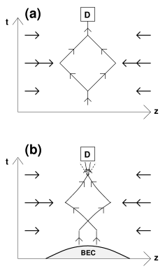
Figure 1: Interferometric loop of the Michelson interferometer with single atoms (a) and with Bose condensates (b).

Between the splitting and recombination pulses the wave function can be approximately decomposed as

$$\psi(z,\,t)\approx$$

$$\quad\frac{1}{\sqrt{2}}\left\{e^{i\phi_{+}(z,\,t)}e^{i(m\bar{v}_{+}(t)z-\bar{\epsilon}_{+}(t)t)/\hbar}\chi(z-\bar{z}_{+}(t))\right.$$

$$\quad\left.+e^{i\phi_{-}(z,\,t)}e^{i(m\bar{v}_{-}(t)z-\bar{\epsilon}_{-}(t)t)/\hbar}\chi(z-\bar{z}_{-}(t))\right\},$$ (11)

where the phases $\phi_{\pm}$ will be shown to be approximately real. Here

$$\bar{z}_{\pm}(t)=\left\{\begin{array}[]{lll}\pm V_{Q}t&\mbox{for}&0<t<T\\ \pm V_{Q}T\mp V_{Q}(t-T)&\mbox{for}&T<t<2T\end{array}\right.$$ (14)

are the classical trajectories, originating at $z=0$, corresponding to the right (+) and left (-) arms of the interferometer;

$$\bar{v}_{\pm}(t)=\dot{\bar{z}}_{\pm}(t)=\left\{\begin{array}[]{lll}\pm V_{Q}&\mbox{for}&0<t<T\\ \mp V_{Q}&\mbox{for}&T<t<2T\end{array}\right.$$ (17)

are the corresponding classical velocities; finally, $\bar{\epsilon}_{+}(t)=\bar{\epsilon}_{-}(t)=E_{Q}\equiv mV_{Q}^{2}/2$ are the corresponding kinetic energies. The velocity $V_{Q}$ is given by $V_{Q}\equiv\hbar Q/m$, where $m$ is the atomic mass.

The resulting differential phase shift

$$\Delta\phi(z)\equiv\phi_{+}(z,\,2T)-\phi_{-}(z,\,2T)$$ (18)

consists of two parts: $\Delta\phi(z)=\Delta\phi_{\text{signal}}+\Delta\phi_{\text{distortion}}(z)$. The first, spatially independent part is the useful signal, related to the effect the interferometer measures. The second part is the result of the distortion caused by unaccounted-for external fields and, in our case, mean-field interactions. The distortion phase shift leads to two effects. The first is a correction to the signal phase shift. This effect can in principle be accounted for, if the nature of the distortion is known. The second effect is a degradation of contrast in the interferometric signal. This degradation can not be eliminated easily if $\Delta\phi_{\text{distortion}}(z)$ changes substantially over the length of the atomic cloud. If both effects are taken into account, then the interferometric signal

$$S(\Delta\phi_{\text{signal}})\equiv N^{-1}\times$$

$$\quad\int_{-\infty}^{+\infty}dz\,\cos^{2}((\Delta\phi_{\text{signal}}+\Delta\phi_{\text{distortion}}(z))/2)|\chi(z)|^{2}$$

can be shown to be

$$S(\Delta\phi_{\text{signal}})=\frac{1}{2}+\frac{M}{2}\cos(\Delta\phi_{\text{signal}}-\delta)\quad,$$

where the fringe contrast $M$ and fringe shift $\delta$ are given by

$$M=\sqrt{A^{2}+B^{2}}$$ (19)

$$\delta=\arg(A,\,B)\quad,$$ (20)

and

$$A=N^{-1}\int_{-\infty}^{+\infty}dz\,\cos(\Delta\phi_{\text{distortion}}(z))|\chi(z)|^{2}$$

$$B=N^{-1}\int_{-\infty}^{+\infty}dz\,\sin(\Delta\phi_{\text{distortion}}(z))|\chi(z)|^{2}\quad.$$

The goal of this paper is to calculate the fringe contrast degradation caused by mean-field interactions, compare the results with the experimentally observed values, and suggest methods for eliminating this degradation.

Analysis of the mean-field effects.– We describe the evolution of the atomic cloud using the nonlinear Schrödinger equation

$$i\hbar\frac{\partial}{\partial t}\psi+\frac{\hbar^{2}}{2m}\frac{\partial^{2}}{\partial z^{2}}\psi=U(z,\,t)\psi+g_{\rm 1D}|\psi|^{2}\psi\quad,$$ (21)

where $U(z,\,t)$ is an external field comprising the object of the measurement and any other auxiliary fields present; $g_{\rm 1D}=-\hbar^{2}/\mu\,a_{\rm 1D}$ is the one-dimensional coupling constant; $a_{\rm 1D}=(-a^{2}_{\perp}/2a)\,[1-{\mathcal{C}}(a/a_{\bot})]$ is the one-dimensional scattering length; $\mu=m/2$ is the reduced mass; $a_{\perp}=\sqrt{\hbar/\mu\,\omega_{\perp}}$ is the size of the transverse ground state of the guide; ${\mathcal{C}}=1.4603\dots$ (see Olshanii ); lastly, $a$ is the three-dimensional $s$-wave scattering length. We further decompose the wave function into a quasi-Fourier series

$$\psi=\frac{1}{\sqrt{2}}\sum_{n=\pm 1,\,\pm 3,\ldots}\psi_{n}\quad,$$ (22)

where each term obeys

$$\left(i\hbar\frac{\partial}{\partial t}+\frac{\hbar^{2}}{2m}\frac{\partial^{2}}{\partial z^{2}}\right)\psi_{n}=$$ (23)

$$\quad U(z,\,t)\psi_{n}+\frac{g_{\rm 1D}}{2}\sum_{n_{2},\,n_{3}}\psi^{\star}_{n_{2}+n_{3}-n}\psi_{n_{2}}\psi_{n_{3}}\quad.$$

The initial condition for the system (23) is given by the result of applying the beamsplitter (10) to the initial condition (1). We get

$$\psi_{\pm 1}(z,\,t=0+)=\chi(z)e^{\pm Qz}$$

$$\psi_{n\neq\pm 1}(z,\,t=0+)=0\quad.$$

Let us assume that the $\psi_{\pm 1}$ components of the wave function remain dominant, as they are initially, and then verify this assumption for self-consistency. Here and throughout the paper we will suppose that the beamsplitter recoil energy $E_{Q}$ is much greater than the mean-field energy $g_{\rm 1D}|\chi|^{2}$:

$$\varepsilon_{{\rm nl}}\sim\frac{g_{\rm 1D}|\chi|^{2}}{E_{Q}}\ll 1\quad.$$ (24)

Under these assumptions the strongest higher harmonics generated are

$$\psi_{\pm 3}=-\frac{1}{16}\frac{g_{\rm 1D}\psi^{\star}_{\mp 1}\psi_{\pm 1}}{E_{Q}}\psi_{\pm 1}\quad,$$ (25)

and it is indeed small provided the parameter (24) is small. Another assumption used to derive (25) was that the beamsplitter recoil energy $E_{Q}$ dominates another energy scale associated with the deviation of the momentum distribution of the dominant harmonics $\psi_{\pm 1}$ from that of strict $\delta$-peaks around $p=\pm\hbar Q$. As we will see from the following, in a realistic experiment this energy scale satisfies an even stricter requirement of being dominated by the “time-of-flight” energy $\hbar/T$.

In general, according to our findings the dynamics of higher harmonics is simply reduced to an adiabatic following of the dominant $\psi_{\pm 1}$ ones. This observation greatly simplifies further analysis. In short, one may safely exclude the couplings to higher harmonics from the equations of evolution for $\psi_{\pm 1}$, obtain results, and add the correction (25) a posteriori.

The equations for the dominant harmonics $\psi_{\pm 1}$ now become

$$\left(i\hbar\frac{\partial}{\partial t}+\frac{\hbar^{2}}{2m}\frac{\partial^{2}}{\partial z^{2}}\right)\psi_{\pm 1}=U_{\pm}(z,\,t)\psi_{\pm 1}\quad,$$ (26)

where the effective potentials for the right (+) and left (-) arms of the interferometer read

$$U_{\pm}(z,\,t)=U(z,\,t)+\frac{g_{\rm 1D}}{2}|\psi_{\pm 1}|^{2}+g_{\rm 1D}|\psi_{\mp 1}|^{2}\quad.$$ (27)

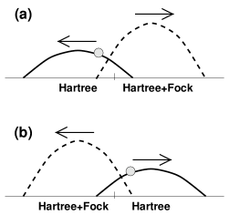
Figure 2: An artistic view of the mean-field effects in a Michelson interferometer. Notice that the mean-field potential is different for the right arm (a) and the left arm (b).

The first part of the mean-field potential is the contribution of the part of the cloud to which the given interferometer arm belongs. The second, twice-as-strong part is the influence of the opposite arm. The factor of two difference between the two contributions (illustrated in Fig. 2) can be traced to the difference between the Hartree-type interaction among atoms in the condensate, and the Hartree-Fock-type interaction between atoms in the condensate and those out of the condensate.

In what follows we study the effect of the mean-field interaction (27) on the differential phase shift (18) and fringe contrast (19).

Differential phase shift.– From now on we will be using the representation (11) for the wave function, where the phase factors $\phi_{\pm}(z,\,t)$ (generally complex) are still unknown. The equation (26) under the representation (11) leads to the following equations for the phase factors

$$\frac{\partial}{\partial\tau_{\pm}}\phi_{\pm}=-U_{\pm}(z,\,t)/\hbar+D_{\pm}(z,\,t)\quad.$$ (28)

Here

$$\frac{\partial}{\partial\tau_{\pm}}\equiv\frac{\partial}{\partial t}+\bar{v}_{\pm}(t)\frac{\partial}{\partial z}\quad;$$ (29)

the classical velocity $\bar{v}_{\pm}$ is given in (17); the potentials (27) are

$$U_{\pm}(z,\,t)=U(z,\,t)$$ (30)

$$\quad+\frac{g}{2}|\chi(z-\bar{z}_{\pm}(t))|^{2}+g|\chi(z-\bar{z}_{\mp}(t))|^{2}\quad;$$

the classical coordinate $\bar{z}_{\mp}(t)$ is represented by (14). Finally, the correction term $D$ is

$$D_{\pm}=D_{J,\,\pm}+D_{{\rm dyn.},\,\pm}+D_{{\rm dyn.-init.},\,\pm}+D_{{\rm init.},\,\pm}\quad,$$ (31)

where

$$D_{J,\,\pm}=i\frac{\hbar^{2}}{2m}\frac{\partial^{2}}{\partial z^{2}}\phi_{\pm}\,,$$ (32)

$$D_{{\rm dyn.},\,\pm}=-\frac{\hbar^{2}}{2m}\left(\frac{\partial}{\partial z}\phi_{\pm}\right)^{2}\,,$$ (33)

$$D_{{\rm dyn.-init.},\,\pm}\,,$$ (34)

$$\quad=i\frac{\hbar}{m}\left(\frac{\partial}{\partial z}\phi_{\pm}\right)\left(\frac{\partial}{\partial z}\ln(\chi(z-\bar{z}_{\pm}(t)))\right)\,,\;\text{and}$$

$$D_{{\rm init.},\,\pm}=\frac{\hbar^{2}}{2m}\frac{\frac{\partial^{2}}{\partial z^{2}}\chi(z-\bar{z}_{\pm}(t))}{\chi(z-\bar{z}_{\pm}(t))}\quad.$$ (35)

Now we decompose the phase shift

$$\phi_{\pm}=\bar{\phi}_{\pm}+\delta\phi_{\pm}$$ (36)

into a sum of the principal part obeying

$$\frac{\partial}{\partial\tau_{\pm}}\bar{\phi}_{\pm}=-U(z,\,t)_{\pm}/\hbar\quad,$$ (37)

and the correction originating from the $D$ term in (28). We assume that the correction $\delta\phi_{\pm}$ is small,

$$\delta\phi_{\pm}\ll 1\quad,$$ (38)

which we will justify later.

Finally the differential phase shift reads

$$\Delta\phi(z)=-\hbar^{-1}\int_{0}^{2T}dt^{\prime}\times$$ (39)

$$\quad\quad\left\{U_{+}(z-\bar{z}_{+}(2T)+\bar{z}_{+}(t^{\prime}),\,t^{\prime})\right.$$

$$\quad\quad\quad\left.-U_{-}(z-\bar{z}_{-}(2T)+\bar{z}_{-}(t^{\prime}),\,t^{\prime})\right\}$$

In what follows we will assume that the initial atomic wave function has the Thomas-Fermi profile

$$\chi(z)=\frac{m\omega_{\rm BEC}^{2}}{2}(R^{2}-z^{2})\theta(R-|z|)$$ (40)

Having in mind certain applications we will also add an external harmonic oscillator potential

$$U(z,\,t)=\frac{m\omega_{0}^{2}}{2}z^{2}$$ (41)

of an arbitrary frequency $\omega_{0}$. We will further classify both as distortion effects and set the useful signal to zero. To the order of approximations we made, the caused by distortion fringe shift and fringe contrast degradation analyzed below are independent of the useful signal, and thus the latter can indeed be omitted. The distortion differential phase shift now becomes equal to the total one: $\Delta\phi_{\text{distortion}}(z)=\Delta\phi(z)$.

Interaction-induced loss of contrast: small interferometers.– First consider the case of small interferometers, where the interferometric arms are substantially overlapped during the whole interferometric cycle, $V_{Q}T\ll R$. In this case we can easily compute the combined mean-field and harmonic-oscillator contribution to the differential phase shift $\Delta\phi$ (see (39)), as well as the resulting fringe contrast $M$ (see 19). They read

$$\Delta\phi_{\text{distortion}}(z)=2Kz\quad$$ (42)

and

$$M=|f(2\tilde{K}R)|\quad.$$ (43)

Here

$$\tilde{K}=m\tilde{\omega}^{2}T^{2}V_{Q}/\hbar$$ (44)

has the meaning of the half of the differential momentum acquired by atoms in the mean field and in the harmonic oscillator field (see Fig. 1(b)),

$$\tilde{\omega}^{2}=2\omega_{\rm BEC}^{2}-\omega_{0}^{2}\quad,$$ (45)

and

$$f(\xi)=3(\sin(\xi)-\xi\cos(\xi))/\xi^{3}\quad.$$ (46)

Here and below $\omega_{\rm BEC}$ is the frequency of the harmonic trap for which the state (40) would be the ground state, and $R$ is the Thomas-Fermi radius. Note that for the configuration considered the fringes are suppressed, but either not shifted at all or shifted by $\pi$ (see (20)). Notice also that for a particular case of $\omega_{0}=\sqrt{2}\omega_{\rm BEC}$ the differential phase shift vanishes and thus the fringe contrast is strictly 100%. We will discuss the implications of this phenomenon below.

The expression (43) for the fringe contrast in small interferometers is the first principal result of this paper.

Remedies for the contrast degradation: small interferometers.– As one can see from (42), the distortion of the differential phase shift in small interferometers disappears completely if the frequency of the external harmonic trap is chosen to be $\sqrt{2}$ higher than the frequency of the mean-field potential:

$$\omega_{0}=\sqrt{2}\,\omega_{\rm BEC}\quad\Rightarrow\quad\Delta\phi_{\text{distortion}}=0\quad.$$ (47)

This can be realized in two ways:

(a) The first scheme is applicable if the longitudinal frequency $\omega$ can be controlled independently of the transverse frequency $\omega_{\perp}$. In this case, one should start by preparing the condensate in the ground state of the longitudinal trap. Then, just before the splitting pulse, one should increase the longitudinal frequency by a factor of $\sqrt{2}$ in a short ramp (Fig. 3(a)).

(b) The second scheme assumes that both longitudinal and transverse frequencies are controlled by the same source, and thus the ratio between them is always the same. Then the change in the longitudinal frequency will affect the nonlinear coupling constant $g$ (to which the square of the condensate frequency $\omega_{\rm BEC}^{2}$ is linearly proportional) due to the simultaneous change in the transverse frequency. Note that $g$ is linearly proportional to $\omega_{\perp}$. In this case one satisfies the condition (47) by increasing, prior to the splitting pulse, both the longitudinal and the transverse frequencies by a factor of 2 (Fig. 3(b)).

Note that both schemes are completely insensitive to possible fluctuations in the number of particles in the condensate.

Interaction-induced loss of contrast: large interferometers.– Consider now the the case of large interferometers where for some period of time during the cycle the arms are totally spatially separated: $V_{Q}T\geq R$. The differential phase shift in this case reads

$$\Delta\phi_{\text{distortion}}(z)=2K_{0}z-z^{3}/l^{3}\quad,$$ (48)

where

$$K_{0}=-m\omega_{0}^{2}T^{2}V_{Q}/\hbar$$ (49)

$$l=(m\omega_{\rm BEC}^{2}/3\hbar V_{Q})^{\frac{1}{3}}\quad.$$ (50)

Notice that unlike in the small interferometer case, for no choice of parameters the differential phase shift can be completely eliminated, and that the contribution from the harmonic potential grows with the time duration of the cycle while the one from the mean-field is stationary. This makes us to believe that for large interferometers the most promising implementation will be the free-space one with no longitudinal confinement present.

In the case of $\omega_{0}=0$ the fringe contrast assumes the following compact expression:

$$M={\cal F}(\eta)\quad,$$ (51)

(see Fig. 4) where

$$\eta = (2m\omega_{\rm BEC}^{2}R^{3}/3\hbar V_{Q})^{\frac{1}{3}}$$ (52)

$$= (g_{\rm 1D}N/\hbar V_{Q})^{\frac{1}{3}}\quad,$$

is the parameter governing the fringe contrast,

$${\cal F}(\eta)=\frac{3}{2}{{}_{1}F_{2}}(1/6;\,1/2,\,7/6;\,-\eta^{6}/16)$$

$$\qquad-\sin(\eta^{3}/2)/\eta^{3}\quad,$$ (53)

and ${}_{n}F_{m}(a_{1},\,\ldots,\,a_{n};\,b_{1},\,\ldots,\,b_{m};\,\xi)$ is the generalized hypergeometric function.

Notice that the parameter $\eta$ depends on neither the shape of the atomic cloud nor on the interferometric cycle duration. For a given set of atomic and waveguide parameters the large contrast requirement $\eta\ll 1$ defines a universal limit for the number of atoms:

$$N\ll\hbar V_{Q}/g_{\rm 1D}\quad,$$ (54)

The expression (51) is the second principal result of our paper.

Figure 3: Two schemes for the preparation of the initial wave packet, designed to eliminate the interatomic-interaction-induced degradation of the fringe contrast in small interferometers. (a) Situation when the longitudinal confinement can be controlled independently from the transverse one. (b) Situation when the longitudinal and transverse confinements are linearly linked one to another.

Figure 4: Fringe contrast ratio vs. the universal parameter $\eta$ for large interferometers.

Limits of the validity of our computational scheme.– In order for our conclusions be valid the correction (38) originating from the neglected terms in the kinetic energy must be small. We have performed a thorough investigation aimed at understanding the physical meaning of the neglected corrections and estimating their value. The results are as follows.

The correction $\delta\phi_{\pm}$ can be decomposed into a sum of four terms

$$\delta\phi_{\pm}=\delta\phi_{J,\,\pm}+\delta\phi_{{\rm dyn.},\,\pm}+$$

$$\qquad\delta\phi_{{\rm dyn.-init.},\,\pm}+\delta\phi_{{\rm init.},\,\pm}$$ (55)

with the following interpretation:

$$e^{\delta\phi_{J,\,\pm}}\approx|J_{U_{\pm}}|^{-\frac{1}{2}}$$ (56)

$$e^{\delta\phi_{{\rm dyn.},\,\pm}+\delta\phi_{{\rm dyn.-init.},\,\pm}+\delta\phi_{{\rm init.},\,\pm}}$$ (57)

$$\quad\approx\langle\chi(z-\bar{z}_{\pm}(t))|e^{-i\int_{0}^{t}dt\,(p_{U_{\pm}}+\hat{p})/2m\hbar}|\chi(z-\bar{z}_{\pm}(t))\rangle.$$

The first correction is related to the expansion factor (Jacobian) of the bunch of trajectories of classical particles moving in the field $U_{\pm}$. The second, third, and forth corrections originate from the neglected kinetic energy, both the initial kinetic energy (coming from the momentum distribution of $\chi$) and that acquired in the field $U_{\pm}$. The above corrections (together with the nonlinear correction (24)) lead to the following requirements for the validity of the approximations used:

$$\varepsilon_{J}=(\tilde{\omega}T)^{2}\ll 1$$ (58)

$$\varepsilon_{{\rm dyn.}}=m\tilde{\omega}^{4}\tilde{z}^{2}T^{3}/\hbar\ll 1$$ (59)

$$\varepsilon_{{\rm init.}}=\hbar T/mR^{2}\ll 1$$ (60)

$$\varepsilon_{{\rm nl}}=(\tilde{\omega}R/V_{Q})^{2}\ll 1\quad,$$ (61)

where $\tilde{z}$ is the typical atomic coordinate, given by $\tilde{z}\sim R$ ($\tilde{z}\sim V_{Q}T$) for small (large) interferometers. For a typical set of parameters of the JILA experiment with $\tilde{\omega}=2\pi\times 3.2\mbox{Hz}$ and $T=10^{-3}\,\mbox{s}$ (corresponding to the small interferometer case), the values of these parameters are indeed small, validating our approximation: $\varepsilon_{J}=\varepsilon_{{\rm dyn.-init.}}=4.1\times 10^{-4}$, $\varepsilon_{{\rm dyn.}}=4.7\times 10^{-4}$, $\varepsilon_{{\rm init.}}=3.6\times 10^{-4}$, and $\varepsilon_{{\rm nl}}=3.6\times 10^{-3}$.

Comparison with the JILA experiment.– The parameters of the JILA’s experiment on Michelson interferometer on a magnetic chip dana lie in the range intermediate between the small and large interferometer regimes and requires no assumption on the distance between the arms $V_{Q}$ vis a vis the cloud size $R$. The equation for the fringe contrast in this case must be integrated numerically. In dana a time- and space-localized pulse of magnetic field was used as the phase signal. A stationary harmonic potential of frequency $\omega_{0}=2\pi\times 5\,\mbox{Hz}$ was present in each realization. The contrast was traced as a function of the duration of the interferometric cycle $2T$, as depicted in Fig. 5. Other parameters read $\omega_{\perp}=2\pi\times 100\,\mbox{Hz}$, $Q=4\pi/\lambda$, where $\lambda=780\,\mbox{nm}$ is the wavelength of light used to produce the interferometric elements, $R=45\,\mu\text{m}$, and $a=100.4\,a_{\text{B}}$. In the experiment the number of atoms varied from one value of the cycle duration to another; these numbers are shown in Fig. 5(a). The value of $\omega_{\rm BEC}$ was extracted from $\omega_{\rm BEC}^{2}=(4/9)g_{\rm 1D}N/mR^{3}$. The results of the comparison are shown at the Fig. 5(a).

One can see from the Fig. 5 that for the parameters chosen the role of interatomic interactions in contrast degradation is relatively small and the main source of the effect is the stationary harmonic trap. This is entirely unexpected since the strength of the interactions was very close to the strength of the trap, typically $\omega_{\rm BEC}^{2}=.25\div.4\omega_{0}^{2}$, and moreover in the small interferometer regime the strength interactions become multiplied by a factor of 2 of Fock origin (see (45). One can show further that the relatively weak role of interactions in the JILA experiment is not related to any small parameter, but is solely an interplay of numerical prefactors. To illustrate this point we show at the Fig. 5(b) a theoretical prediction for $N=4.5\times 10^{4}$ atoms exhibiting a dominant role of the interatomic interactions.

Figure 5: Fringe contrast ratio vs. duration of the interferometric cycle corresponding to the parameters of the JILA experiment with Michelson interferometer on a chip, with magnetic gradient as the phase element. (a) Curves correspond to $N=3.\times 10^{3}$ atoms, the as same 4 ms point in the experiment. The theoretical predictions for the actual experimental numbers of atoms at every run are also shown. (b) The same as (a), but for $N=4.5\times 10^{4}$ atoms, where a reduction of the fringe contrast to 50% is expected.

Summary and outlook.–

(1) We have developed a simple computational scheme that allows to include the effect of interatomic interactions in calculation of fringe shift and fringe degradation in waveguide based atom interferometers.

(2) In two cases we have found simple analytic expression for fringe contrast. These cases are: small interferometers where the spatial separation between the arms is much smaller than the atomic cloud size, $V_{Q}T\ll R$; and large interferometers where at at least one instance the arms are fully separated, $V_{Q}T\geq R$.

(3) In the case of small interferometers the analytic expression for the contrast degradation allowed us to suggest a simple recipe canceling the destructive effect of interactions completely.

(4) In the case of large interferometers the effect of interactions can not, to our knowledge, be canceled entirely. Furthermore, the interatomic interactions set an universal limit on the number of atoms involved in the interferometric process: $N\ll\hbar V_{Q}/g_{\rm 1D}$. Notice that this bound depends on the characteristics of the atom and the waveguide only (where the “beam-splitter velocity” $V_{Q}$ is supposed to be linked to the atomic transition frequency), while neither the timing of cycle nor the size of the atomic cloud enter.

(5) Using the method developed we have analyzed the results of the recent JILA experiment on Michelson interferometer on atom chip. In spite of comparable strength of interatomic interactions and stationary longitudinal trap present in the experiment, our results indicate a relatively weak role of interactions in fringe contrast degradation. This finding is can not be traced to any small parameter, but is a mere interplay of numerical prefactors. A moderate ten-fold increase (to $N=4.5\times 10^{4}$) in the number of atoms will reduce, for large interferometer case, the fringe visibility to 50%, even without an additional longitudinal trap present, reflecting the universal limit outlined above.

(6) Michelson interferometer is a closed-loop white-light scheme by design; it is supposed to produce clear fringes even for input sources with a short coherence length. As one can see from the Fig. 2(b), the mean-field pressure leads to two distinct effects. The first effect is the change in the relative momentum of the interferometer arms; this is what we addressed in the present work. The second effect is the distortion of the interferometric path, as a result of which the path becomes open, and thus the interferometer becomes sensitive to the longitudinal coherence. For zero-temperature condensates this does not lead to any loss of contrast. At finite temperature the degradation due to the broken interferometer loop becomes relevant, and we are going to study this effect in the nearest future.

- (1) Atom Interferometry, edited by P. R. Berman (Academic, New York, 1997).
- (2) O. Carnal and J. Mlynek, Phys. Rev. Lett. 66, 2689 (1991).
- (3) D. W. Keith, C. R. Ekstrom, Q. A. Turchette, and D. E. Pritchard, Phys. Rev. Lett. 66, 2693 (1991).
- (4) M. Kasevich and S. Chu, Phys. Rev. Lett. 67, 181 (1991).
- (5) J. E. Simsarian, J. Denschlag, M. Edwards, C. W. Clark, L. Deng, E. W. Hagley, K. Helmerson, S. L. Rolston, and W. D. Phillips, Phys. Rev. Lett. 85, 2040 (2000).
- (6) Y. Torii, Y. Suzuki, M. Kozuma, T. Sugiura, T. Kuga, L. Deng, and E. W. Hagley, Phys. Rev. A61, 041602 (2000).
- (7) B. P. Anderson, M. A. Kasevich, Science 282 1686 (1998).
- (8) D. Hellweg, L. Cacciapuoti, M. Kottke, T. Schulte, K. Sengstock, W. Ertmer, J. J. Arlt, Phys. Rev. Lett. 91, 010406 (2003).
- (9) Artur Widera, Olaf Mandel, Markus Greiner, Susanne Kreim, Theodor W. H nsch, and Immanuel Bloch, Phys. Rev. Lett. 92, 160406 (2004).
- (10) Y. Shin, M. Saba, T. A. Pasquini, W. Ketterle, D. E. Pritchard, A. E. Leanhardt, Phys. Rev. Lett. 92, 050405 (2004).
- (11) Ying-Ju Wang, Dana Z. Anderson, Victor M. Bright, Eric A. Cornell, Quentin Diot, Tetsuo Kishimoto, Mara Prentiss, R. A. Saravanan, Stephen R. Segal, Saijun Wu, Phys. Rev. Lett. 94, 090405 (2005).
- (12) P. K. Rekdal, S. Scheel, P. L. Knight, E. A. Hinds, Phys. Rev. A 70, 013811 (2004).
- (13) C. J. Vale, B. Upcroft, M. J. Davis, N. R. Heckenberg, H. Rubinsztein-Dunlop, J.Phys. B 37 2959 (2004).
- (14) S. Schneider, A. Kasper, Ch. vom Hagen, M. Bartenstein, B. Engeser, T. Schumm, I. Bar-Joseph, R. Folman, L. Feenstra, and J. Schmiedmayer, Phys. Rev. A 67, 023612 (2003).
- (15) H. Ott, J. Fortagh, G. Schlotterbeck, A. Grossmann, and C. Zimmermann, Phys. Rev. Lett. 87, 230401 (2001).
- (16) W. H nsel, P. Hommelhoff, T. W. H nsch, and J. Reichel, Nature (London) 413, 498 (2001).
- (17) M. Vengalattore, W. Rooijakkers, and M. Prentiss, Phys. Rev. A 66, 053403 (2002).
- (18) A. Rohrl, M. Naraschewski, A. Schenzle, H. Wallis, Phys. Rev. Lett. 78, 4143 (1997).
- (19) M. D. Girardeau, K. K. Das, E. M. Wright, Phys. Rev. A66, 023604 (2002).
- (20) S. Chen and R. Egger, Phys. Rev. A68, 063605 (2003).
- (21) J. A. Stickney and A. A. Zozulya, Phys. Rev. A 66, 053601 (2002).
- (22) Saijun Wu, Yingju Wang, Quentin Diot, Mara Prentiss, e-print physics/0408011.
- (23) M. Olshanii, Phys. Rev. Lett. 81, 938 (1998).