Bose-Fermi Mixtures Near an Interspecies Feshbach Resonance:
Testing a Non Equilibrium Approach

Abstract

We test a non equilibrium approach to study the behavior of a Bose-Fermi mixture of alkali atoms in the presence of a Feshbach resonance between bosons and fermions. To this end we derive the Hartree-Fock-Bogoliubov (HFB) equations of motion for, the interacting system. This approach has proven very successful in the study of resonant systems composed of Bose particles and Fermi particles. However, when applied to a Bose-Fermi mixture, the HFB theory fails to identify even the correct binding energy of molecules in the appropriate limit. Through a more rigorous analysis we are able to ascribe this difference to the peculiar role that bosonic depletion plays in the Bose-Fermi pair correlation, which is the mechanism through which molecules are formed. We therefore conclude that molecular formation in Bose-Fermi mixtures is driven by three point and higher order correlations in the gas, unlike any other resonant system studied in the context of ultra-cold atomic physics.

I Introduction

Feshbach resonances have been recently discovered in ultracold mixtures of bosonic fermionic alkali atoms jin ; ketterle . Together with the achievement of degenerate states of such systems inguscio ; ketterle2 ; jin2 , this experimental feat has opened investigative opportunities for the study of new ultracold regimes. From the theoretical point of view, on the other hand, studies of Bose-Fermi mixtures to date have been mostly limited to non resonant physics, focusing mainly on mean field effects in trapped systems roth ; roth2 ; modugno ; hu ; liu ; adh ; buc , phases in optical lattices albus ; lewen ; roth3 ; sanp , or equilibrium studies of homogeneous gases, focusing mainly on phonon induced superfluidity or beyond-mean-field effects stoof1 ; heise ; efre ; vive ; matera ; gardiner .

This paper introduces a time dependent theory of the Bose-Fermi mixture that accounts for the resonant interaction. In systems where the resonant interaction is between two bosons holland_mol ; stoof2 ; oxford or between two fermions holland_ren ; stoof3 ; victor ; griffin ; sasha1 ; oxford1 , the theory of “resonant superfluidity” has already been articulated. This theory is, so far, a big success. In the Bose case, it quantitatively describes the coherent conversion of bosonic atoms into bosonic molecules and back. Indeed, Ramsey interferometry on this system, coupled with this theoretical analysis, has produced the most accurate interaction potentials yet between ultracold rubidium atoms claussen . In the Fermi case, the theory has produced important qualitative insights into the crossover regime between weakly-interacting Cooper pairs on the one hand, and Bose-condensed molecules on the other holland_ren ; stoof3 ; victor ; griffin ; sasha1 ; sasha2 ; oxford1 ; oxford2 .

It seems worthwhile, therefore, to adapt the same level of theory to the resonant Bose-Fermi mixture. In this paper we formulate the problem by writing down the relevant equations of motion at the level of Hartree-Fock-Bogoliubov (HFB) approximation. The equation of motion are suitably number- and energy-conserving, as are their counterparts in boson of fermion systems. However, in sharp contrast to these systems, the HFB theory applied to the Bose-Fermi resonance does not provide quantitatively reasonable results. Specifically we show, by direct numerical solution that the theory cannot reproduce the binding energy of a Bose-Fermi molecule, even in the limit of low density.

The source of this difficulty lies in the approximate treatment of three-body correlations in the theory. The molecules, after all, are composed of two atoms, so the atom-atom-molecule correlation function is of central importance in determining properties of the resulting molecules. In the HFB theory, this three-body correlation function is approximated in terms of two-body correlation functions, which is adequate for Bose-Bose and Fermi-Fermi resonances, but not for the Bose-Fermi mixture. Ultimately, the critical missing piece will turn out to involve the non condensed bosonic atoms.

This paper is organized as follows: We begin our discussion in section II by introducing the Hamiltonian of the system, and justifying such choice. We then proceed to outline the Bogoliubov-Born-Green-Kirkwood-Yvon (BBGKY) formalism used to derived the HFB equations of motion, and show the form they take in free space. In section III we present our results, by first analyzing the equations by physical and analytical insight, and then presenting numerical results in support of our conclusions.

Section LABEL:sec4 approaches the problem from an alternative, perturbative point of view, relevant to low fermionic densities. From this analysis it is clear that molecular binding energies will not be recovered without adequately accounting for the non condensed bosons, thus pointing to their need for a higher-order theory.

II Theoretical Formalism

II.1 The Hamiltonian

We are interested primarily in the effects of resonant behavior on the otherwise reasonably understood properties of the system. To this end we use a model which, in the last few years, has become one of the standards in the literature, and which was used to study the effect of resonant scattering in systems composed of bosons holland_mol ; stoof2 ; oxford , and fermions holland_ren ; stoof3 ; victor ; griffin ; sasha1 ; sasha2 . Because there is already a significant literature explaining the details involved in the choice of the appropriate model Hamiltonian, we only outline the extent of the approximation involved in such a choice.

An accurate approach to the problem would have to incorporate several scattering channels, since the resonance in question is a consequence of the intertwined behavior of the complex internal structures of the atoms. In a field theoretical sense, that would imply having to consider vector fields for the bosons and fermions with as many components as there are spin states involved in the interaction, and a non local interaction tensor of adequate size, to account for all coupling between such components. Fortunately, if we assume that the resonances in the system are sufficiently far from each other, such that it is possible to define a “background,” or away from resonance behavior, we can focus on only one resonance at a time, which in turn makes it possible for an effective two channel model to describe the resonance. Furthermore, since the closed channel threshold is energetically unaccessible at the temperatures of interest, we can “integrate out” the closed channel components of the fermion and boson field, in favor of a fermion fields which we identify as representative of the motion of one boson and one fermion, and which we dub the “molecular field.” In the appropriate limit the molecular field identifies bound states between fermions and bosons. We emphasize that the molecular field is a theoretical artifice that alleviates the need to treat relative motion of two atoms on the natural scale of the interaction (tens of Bohr radii). However, this model is appropriate for the study of the systems at hand, typically composed of $10^{12}$ ${}^{40}K$ atoms per cubic centimeter, whereby the characteristic length scales associated with the many body system are of the order of the inverse Fermi wavenumber, (thousands of Bohr radii), and the average interparticle spacing (tens of thousands Bohr radii), which is given by $({3\over 4\pi\rho})^{1/3}$, where $\rho$ is the atomic density. Lastly, since the coupling terms in the Hamiltonian represent an effective interaction, we can choose its functional form, and we do so by choosing to deal with contact interactions, which simplify the calculations immensely.

The resulting Hamiltonian has the following form:

$$H=H_{0}+H_{I},$$ (1)

where

$$H_{0} = \sum_{p}\epsilon_{p}^{F}\ \hat{a}_{p}^{\dagger}\hat{a}_{p}+\sum_{p}\epsilon_{p}^{B}\ \hat{b}_{p}^{\dagger}\hat{b}_{p}+\sum_{p}\left(\epsilon_{p}^{M}+\nu\right)\ \hat{c}_{p}^{\dagger}\hat{c}_{p}$$

$$+ {\gamma\over 2V}\sum_{p,p^{\prime},q}\hat{b}_{p-q}^{\dagger}\hat{b}_{p^{\prime}+q}^{\dagger}\hat{b}_{p}\hat{b}_{p^{\prime}}$$

$$H_{I} = {V_{bg}\over V}\sum_{p,p^{\prime},q}\hat{a}_{p-q}^{\dagger}\hat{b}_{p^{\prime}+q}^{\dagger}\hat{a}_{p}\hat{b}_{p^{\prime}}$$

$$+ {g\over\sqrt{V}}\sum_{q,p}(\hat{c}_{q}^{\dagger}\hat{a}_{-p+q/2}\hat{b}_{p+q/2}+h.c.).$$

Here $\hat{a}_{p},\hat{b}_{p}$, are the annihilator operators for, respectively, fermions and bosons, $\hat{c}_{p}$ is the annihilator operator for the molecular field holland_ren ; sasha1 ; sasha2 ; $\gamma=4\pi a_{b}/m_{b}$ is the interaction term for bosons, where $a_{b}$ is the boson-boson scattering length; and $V_{bg},\nu$, and $g$ are parameters related to the Bose Fermi interaction, yet to be determined. Also we define single particle energies $\epsilon^{\alpha}=p^{2}/2m_{\alpha}$, where $m_{\alpha}$ indicates the mass of bosons, fermions, or pairs, and $V$ as the volume of a quantization box with periodic boundary conditions.

II.2 Two Body Scattering Parameters

The first step is to find the values for $V_{bg},\nu,g$, in terms of measurable parameters. We will, for this purpose, calculate the 2-body T-matrix resulting from the Hamiltonian in eq. LABEL:act-bfm. Integrating the molecular field out of the real time path integral, negele leads to the following Bose-Fermi interaction Hamiltonian

$$H_{I}^{2body}={1\over V}\left(V_{bg}+{g^{2}\over E-\nu}\right)\sum_{p}\hat{a}_{p}^{\dagger}\hat{b}_{-p}^{\dagger}\hat{a}_{p}\hat{b}_{-p}.$$ (3)

This expression is represented in center of mass coordinates, and $E$ is the collision energy of the system. From the above equation we read trivially the zero energy T-matrix in the saddle point approximation

$$T=(V_{bg}-{g^{2}\over\nu}),$$ (4)

which corresponds to the Born approximation, and we proceed to match it to the conventional parameterization holland_ren ; stoof2

$$T(B)={2\pi\over m_{bf}}a_{bg}\left(1-{\Delta_{B}\over(B-B_{0})}\right),$$ (5)

where $a_{bg}$ is the value of the scattering length far from resonance, $\Delta_{B}$ is the width, in magnetic field, of the resonance, $m_{bf}$ is the reduced mass, and $B_{0}$ is the field at which the resonance is centered.

The identification of parameters between eqns, (4) and (5) proceeds as follows: far from resonance, $|B-B_{0}|>>\Delta_{B}$, the interaction is defined by a background scattering length, via $V_{bg}={2\pi a_{bg}\over m_{bf}}$. To relate magnetic field dependent quantity $B-B_{0}$ to its energy dependent analog $\nu$, requires defining a parameter $\delta_{B}=\partial\nu/\partial B$, which may be thought of as a kind of magnetic moment for the molecules. It is worth noting that $\nu$ does not represent the position of the resonance nor the binding energy of the molecules, and that, in general $\delta_{B}$ is a field-dependent quantity, since the molecular binding energy approaches threshold quadratically. For current purposes we identify $\delta_{B}$ by its behavior far from resonance, where it is approximately constant. Careful calculations of scattering properties using the model in eq. (LABEL:act-bfm), however, leads to the correct Breit-Wigner behavior of the 2-body T-matrix, as we show in section IV

Finally we get the following identifications:

$$V_{bg}={2\pi a_{bg}\over m_{bf}}$$

$$g=\sqrt{V_{bg}\delta_{B}\Delta_{B}}$$

$$\nu=\delta_{B}(B-B_{0}).$$

For our calculations we use the 511G resonance in the ⁴⁰K-⁸⁷Rb system, the parameters we use in the calculations to follow are $a_{bg}=-202a_{0}$, $\delta_{B}=5.1\times 10^{-5}$ K/G, and $\Delta_{B}=1$G.

II.3 The Formalism

We now move on to the many body analysis, and derive the Heisenberg equations of motion for the many body system. The way this is done, is to find equation of motion for correlation functions, $f_{s}(x_{1},....x_{s})$, which represent the probability of finding $s$ particles at positions $x_{1},...,x_{s}$. As it turns out, the equation of motion for the correlation function $f_{1}$ will depend on the function $f_{2}$, which in turn will depend on $f_{3}$, and so on all the way to $f_{N}$, where $N$ is the total number of particles in the system. This is known as a Bogoliubov-Born-Green-Kirkwood-Yvon (BBGKY) hierarchy huang . In practice we will be concerned with momentum space correlation functions, but the idea is the same.

Given the large number of particles in the system, it is impossible to calculate equation of motions for all correlation functions, and we need to invoke an approximation. In practice, correlation functions are often calculated only up to two-body correlations, $s=2$. This is justified under the assumption that interactions are suitably “weak.” Higher-order correlations are included in an approximate way by considering, not the actual atomic constituents, but rather combinations called quasiparticles. The quasiparticles are defined to be noninteracting, so that their higher-order correlation functions can be written in terms of second order correlation functions negele .

Using this qualitative idea we proceed to develop a more formal understanding. In statistical field theory, given an operator $\mathcal{O}$, and Hamiltonian $H$, we define the thermal average of $\mathcal{O}$ with respect to $H$ as $<\mathcal{O}>_{H}=1/ZTr\left\{\mathcal{O}e^{-\beta H}\right\}$, where $\beta=(k_{B}T)^{-1}$ is the inverse temperature, and $Z=Tr\left\{e^{-\beta H}\right\}$ is the partition function. In this framework, the 1-particle correlation function is defined as the thermal average of the number operator, with respect to the Hamiltonian of the system.

In the quasi-particle representation, we define the annihilation operator for quasi-particles as $\alpha$, reminding ourselves that it is a complicated function of $a,a^{\dagger},b,b^{\dagger},c,c^{\dagger}$. In momentum space, the 1-particle correlation function in this representation, will then be $<\alpha_{p1}\alpha_{p2}>_{H_{qp}}$, where $H_{qp}$ is the (noninteracting) quasi-particle Hamiltonian.

Now we introduce the real approximation, namely that the quasi-particles can be written as linear combinations of all possible products of two operators (except for averages involving one fermionic and one bosonic operator, which are easily shown to vanish). The procedure is then to find the Heisenberg equations of motion for these pairs of operators, and then averaging over the quasi-particle Hamiltonian

$$i\hbar{\partial\over\partial t}<\mathcal{O}>_{H_{qp}}=<[\mathcal{O},H]>_{H_{qp}},$$ (7)

which being Gaussian allows us to invoke Wick’s theorem to decompose all higher order correlations in 1-particle correlations, thus truncating the BBGKY hierarchy.

II.4 The Equations of Motion

Before generating Heisenberg equations, we need to take a little care in the treatment of the Bose field, to properly treat the condensed part. To this end we perform the usual separation of mean-field and fluctuations of the Bose field, substituting $b_{0}$ ( the zero-momentum component of the Bose gas) with a c-number $\phi=<b_{0}>_{H_{qp}}$ , and identifying it with the condensate amplitude, while $<b_{p\neq 0}>_{H_{qp}}=0$ are the fluctuations. We insert these definitions in the Hamiltonian in eq. (LABEL:act-bfm), then proceed to calculate commutators.

Since we wish to limit our analysis to a homogeneous gas, we note that the correlation functions $f_{1}(x,x^{\prime})$ can be written in terms of a relative coordinate $y=x-x^{\prime}$. Thus in momentum space $f_{1}(p)$ is the probability to find a particle with momentum p in the gas, or in other words it is the momentum distribution of the system.

Having taken all appropriate commutators, and applied Wick’s theorem, (for more details on the procedure see burnett , or Appendix A for the derivation of a sample equation.), we obtain the following self consistent set of equations of motion for the system:

$$i\hbar{\partial\over\partial t}\phi = V_{bg}\rho_{F}\phi+\gamma\ (2\phi\tilde{\rho}_{B}+\Delta_{B}\phi^{*})+g\rho_{MF}^{*}+\gamma|\phi|^{2}\phi$$ (8.a)

$$\hbar{\partial\over\partial t}\tilde{\eta}(p) = 2\gamma\ \Im m\left[\kappa_{B}(p)(\phi^{*^{2}}+\Delta_{B}^{*})\right]$$ (8.b)

$$i\hbar{\partial\over\partial t}\kappa_{B}(p) = \left[\epsilon_{P}^{B}+2V_{bg}\rho_{F}+4\gamma(|\phi|^{2}+\tilde{\rho_{B}})\right]\kappa_{B}(p)+\gamma(2\tilde{\eta_{B}}(p)+1)(\phi^{2}+\Delta_{B})$$ (8.c)

$$\hbar{\partial\over\partial t}\eta_{F}(p) = -2g\ \Im m(\phi\eta_{MF}(p))$$ (8.d)

$$i\hbar{\partial\over\partial t}\kappa_{F}(p) = \left[\epsilon_{p}^{F}+2V_{bg}(\tilde{\rho_{B}}+|\phi|^{2})\right]\kappa_{F}(p)$$ (8.e)

$$\hbar{\partial\over\partial t}\eta_{M}(p) = 2g\ \Im m(\phi\eta_{MF}(p))$$ (8.f)

$$i\hbar{\partial\over\partial t}\kappa_{M}(p) = \left[\epsilon_{P}^{M}+\nu\right]\kappa_{M}(p)$$ (8.g)

$$i\hbar{\partial\over\partial t}\eta_{MF}(p) = \left[\epsilon_{p}^{F}-\epsilon_{p}^{M}-\nu+V_{bg}(\tilde{\rho_{B}}+|\phi|^{2})\right]\eta_{MF}(p)-g\phi^{*}\left(\eta_{F}(p)-\eta_{M}(p)\right)$$ (8.h)

$$i\hbar{\partial\over\partial t}\kappa_{MF}(p) = \left[\epsilon_{p}^{F}+\epsilon_{p}^{M}+\nu+V_{bg}(\tilde{\rho_{B}}+|\phi|^{2})\right]\kappa_{MF}(p)-g\left[\phi\kappa_{F}(p)+\phi^{*}\kappa_{M}(p)\right],$$ (8.i)

where $\tilde{\eta_{B}}(p)=<b_{p\neq 0}^{\dagger}b_{p\neq 0}>_{H_{qp}}$ is the momentum distribution of non-condensed bosons, and $\tilde{\rho}_{B}=\int{dp\over 2\pi^{2}}p^{2}\tilde{\eta_{B}}(p)$ is the density of non-condensed bosons; $\kappa_{B}(p)=<b_{p\neq 0}b_{p\neq 0}>_{H_{qp}}$ is the anomalous distribution of bosonic fluctuations, and $\Delta_{B}=\int{dp\over 2\pi^{2}}p^{2}\kappa_{B}(p)$ the anomalous density. Similarly $\eta_{F,M}(p)$ are the fermionic and molecular distributions, $\rho_{M,F}$ the densities, and $\kappa_{F,M}(p)$, and $\Delta_{F,M}$ the anomalous molecular and fermionic distributions and densities. Finally $\eta_{MF}(p)=<c_{p}^{\dagger}a_{p}>_{H_{qp}}$ and $\kappa_{MF}(p)=<c_{p}a_{p}>_{H_{qp}}$ are the normal and anomalous distribution for molecule-fermion correlation, with the associated densities $\rho_{MF}$ and $\Delta_{MF}$.

III Analysis and Results

Equations (8.a-8.i) describe the complete self-consistent set of HFB equations for the resonant BF mixture. Inspection of these equations, however, allows us to simplify the set quite dramatically, without sacrificing almost any of the physics thereby contained. First, we notice that the evolution of the anomalous fermionic densities $\kappa_{MF}(p)$, $\kappa_{F}(p)$, and $\kappa_{M}(p)$ is entirely decoupled from the evolution of all other quantities, and can therefore be considered separately. This implies that, since we are mainly interested in the evolution of the normal densities, we can eliminate without approximation all the anomalous ones.

The next thing we notice is that the evolution of the normal and anomalous bosonic averages is completely independent of the resonant interaction, and is controlled only by the background interactions between bosons and with fermions. For typical background interaction strengths, and cold enough temperatures, it is well established that quantum depletion is minor, and the system is well described at the Gross-Pitaevskii level of approximation.

We can therefore write the following reduced set of equations:

$$i\hbar{\partial\over\partial t}\phi = (V_{bg}\rho_{F}+\gamma|\phi|^{2})\phi+g\rho_{MF}^{*}$$ (9.a)

$$\hbar{\partial\over\partial t}\eta_{F}(p) = -2g\ \Im m(\phi\eta_{MF}(p))$$ (9.b)

$$\hbar{\partial\over\partial t}\eta_{M}(p) = 2g\ \Im m(\phi\eta_{MF}(p))$$ (9.c)

$$i\hbar{\partial\over\partial t}\eta_{MF}(p) = \left[\epsilon_{p}^{F}-\epsilon_{p}^{M}-\nu+V_{bg}|\phi|^{2}\right]\eta_{MF}(p)-g\phi^{*}\left(\eta_{F}(p)-\eta_{M}(p)\right).$$ (9.d)

Together with the prospect of simulating time dependent experiments, such a set of equations allow us to calculate many characteristics of the system, which we could use to understand further physics or, more importantly at this stage, to test the theory against our knowledge of the system in various limits.

A relevant quantity we can calculate to this end is the binding energy of the molecules. This can be done by an instantaneous jump of the detuning from large and positive values, where we know the equilibrium distributions very well, to some other arbitrary value. The system thus perturbed oscillates at a specific characteristic frequency, which identifies as the (unique) pole of the HFB many body T-matrix of the system. For negative detunings, as shown below, this pole corresponds to the binding energy of the molecules, dressed by the interactions in the system.

Figure 1 shows a representative example of time evolution of the condensate population (number conservation guarantees that all three populations oscillate with the same frequency) under the conditions described above. In this particular example, at time t=0 the detuning is suddenly shifted to $-5.110^{-6}K$, corresponding to a magnetic field detuning of approximatively $.1G$. The response of the population shows an envelope function, indicated by the gray shaped area, that arises from nonlinearities in the equations of motion. The inset shows that under this envelope is a well defined sinusoidal oscillation.

The nearly monochromatic character of the response is made clear by Fourier transforming the time dependent population. The Fourier Transform shown in the second panel of Fig 1 is strongly peaked at $5.4\times 10^{-6}K$. Similarly, the position of the peak in the frequency spectrum, for different final detunings, should map the molecular binding energy as a function of magnetic field.

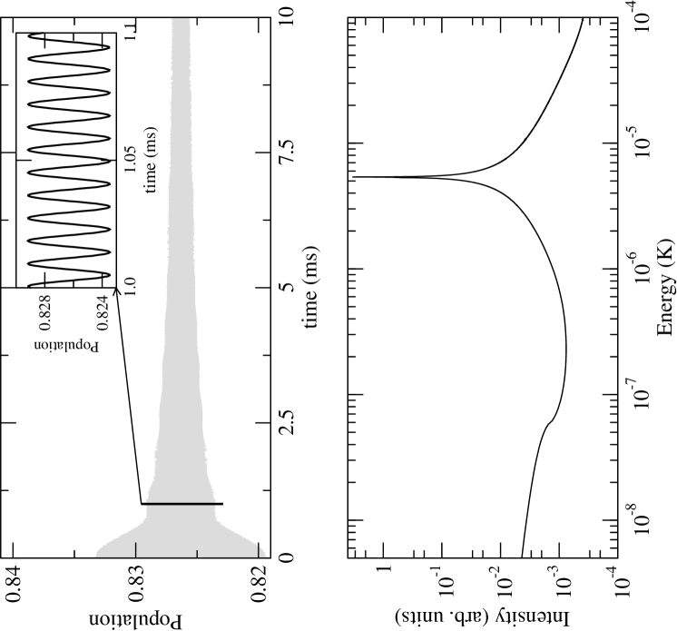
Figure 1: The top panel represents the time evolution of the population of condensed atoms after detuning is suddenly shifted from infinitely positive to -5.1 K ($-.1G$ magnetic detuning). The bottom panel shows the absolute value of Fourier transform of said time evolution. the main peak in this graph represents the computed value of the binding energy, which we see is about $5.410^{-6}K$. The system under consideration is composed of fermionic densities of $10^{12}cm^{-3}$, for a constant density ratio of five bosons per fermion.

Figure 2 shows the results obtained by this method. This plot represents the binding energy of the molecules, dressed by the interactions in the system. This dressing is expected to be weaker for smaller densities of atoms and molecules. In this limit, we should thus recover the two body molecular binding energy, which can be calculated quite accurately from two body close coupling calculations (solid line in fig 2). Instead we see that the pole behavior approaches the bare detuning (dashed line in fig 2), indicating that the renormalization of the binding energy obtained at the presented level of approximation is inadequate to correctly include the two-body physics. This behavior is in sharp contrast to the Bose-Bose resonant interaction, where the correct binding energy is preserved at the HFB level holland_mol . This is also true for the Fermi-Fermi case holland_priv .

This discrepancy is due to the fact that the creation of molecules requires the formation of correlations between bosons and fermions, which, as shown in the following, cannot exist if the density matrix is assumed to be Gaussian. Specifically what is required is a more careful consideration of the noncondensed bosons

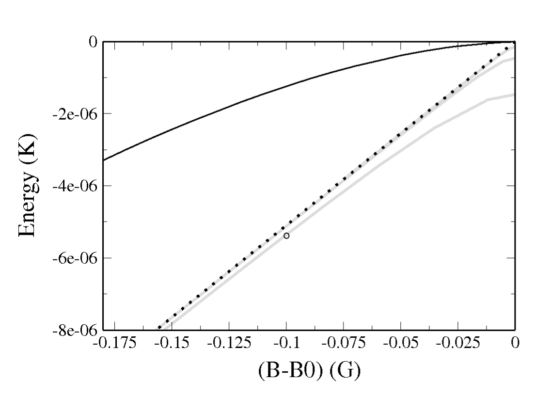
Figure 2: Plot representing the poles of the scattering t-matrix for the 511G ${}^{87}Rb$ - ${}^{40}K$ Feshbach resonance. The dotted line represents the “bare” molecular detuning as a function of field, as defined in the text. The solid black line is the correct binding energy of the molecular state, obtained by means of full close coupling calculations, while the gray solid lines are the eigenenergies obtained from equations 9.a-9.d, for different atomic densities. From top to bottom on the right the grey lines refer to fermionic densities of $10^{10}cm^{-3}$,$10^{11}cm^{-3}$, and $10^{12}cm^{-3}$, for a constant density ratio of five bosons per fermion. We note that for lower and lower densities the calculated binding energy incorrectly approaches the bare detuning instead of the correct two-body binding energy.

IV The Importance of Bosonic Depletion

The reason for the failure of the HFB theory is not immediately clear from the theory itself. To bring out the inadequacy of this theory in the dilute limit, we now recast the problem in an alternative perturbative form that can reproduce the correct behavior in the two body limit. This path integral approach will also lay bare the role of noncondensed bosons.

What we will see in the upcoming analysis may be qualitatively understood in the following simple terms. A molecule in the gas can decay into a pair of “virtual” (i.e. non energy conserving) atoms, which can then meet again and reform the molecule. The incidence of these events modifies the behavior of the molecule, and an appropriate treatment of these virtual excitations is therefore necessary to correctly include the two body properties of the molecules in the many body theory. In particular, the molecules can decay forming a virtual non condensed boson, and the contribution of this set of events to the physics of the molecules turns out to be very important. An appropriate theory would therefore consider the coupling of the molecules to non condensed bosons explicitly, which implies that one has to include in the equations of motion three point averages, such as $<c^{\dagger}_{q}a_{-p+q/2}b_{(p+q/2)}>$. Since the HFB theory disregards three point averages, it only contains molecule-atom-atom couplings of the form $<c^{\dagger}_{q}a_{q}>\phi_{0}$, where molecules can only decay forming a condensed boson.

It is straightforward to see that the HFB theory treats 3-body correlation functions differently depending on the quantum statistics of the constituents. For a Bose-Bose mixture, the correlation function is approximated (schematically) by

$$\langle bbm\rangle\approx\langle m\rangle\langle b(-q)b(q)\rangle+2\langle b\rangle\langle bm\rangle.$$ (10)

The first term of the right of this expression allows explicitly for virtual bosonic pairs of arbitrary momentum, provided that the molecular field $\langle m\rangle$ accounts for most of the molecules, which is assumed to be the case. Similarly, in a mixture of distinct fermions, the correlation function reads

$$\langle f_{1}f_{2}m\rangle\approx\langle m\rangle\langle f_{1}(q)f_{2}(-q)\rangle,$$ (11)

and the same argument applies, since the molecules are bosons.

For the Bose-Fermi mixture, on the other hand, the correlation function would be approximated by

$$\langle bfm\rangle\approx\langle b\rangle\langle fm\rangle+\langle f\rangle\langle bm\rangle+\langle m\rangle\langle bf\rangle.$$ (12)

The required virtual atom-atom pairs would arise from the third term on the right-hand-side of this expression. However, these molecules are fermions, which have no mean field, $\langle m\rangle=0$. The only surviving term is then the first one, which accounts only for condensed bosons, and somehow correlates the fermionic atoms to the fermionic molecules. This is only an indirect way to get the bosons and fermions correlated.

IV.0.1 Two-Body Scattering

The perturbative analysis begins by recasting the Hamiltonian in eq. (LABEL:act-bfm) in terms of a 2-body action, in center of mass coordinates :

$$S[\psi,\psi^{\dagger},\phi,\phi^{\dagger},\xi,\xi^{\dagger}]=S_{B}[\phi,\phi^{\dagger}]+S_{F}[\psi,\psi^{\dagger}]+S_{M}[\xi,\xi^{\dagger}]+S_{C}[\psi,\psi^{\dagger},\phi,\phi^{\dagger},\xi,\xi^{\dagger}],$$ (13)

where the field $\phi$ represents the bosons, $\psi$ the fermions, and $\xi$ the fermionic molecules, and where

$$S_{B}[\phi,\phi^{\dagger}] =\int{d\omega\over 2\pi}\sum_{\bf p}(-\hbar\omega+\epsilon_{p}^{B})\ \phi^{\dagger}_{\omega,{\bf p}}\phi_{\omega,{\bf p}}+{1\over 2V}\gamma\int{d\omega\over 2\pi}\sum_{{\bf p},{\bf p^{\prime}}{\bf q}}\phi_{\omega,{\bf p}-{\bf q}}^{\dagger}\phi_{\omega,{\bf p^{\prime}}+{\bf q}}^{\dagger}\phi_{\omega,{\bf p^{\prime}}}\phi_{\omega,{\bf p}}$$ (14)

$$S_{F}[\psi,\psi^{\dagger}] =\int{d\omega\over 2\pi}\sum_{\bf p}(-\hbar\omega+\epsilon_{p}^{F})\ \psi^{\dagger}_{\omega,{\bf p}}\psi_{\omega,{\bf p}}$$

$$S_{M}[\xi,\xi^{\dagger}] =\int{d\omega\over 2\pi}\sum_{\bf p}(-\hbar\omega+\epsilon_{p}^{M}+\nu)\ \xi^{\dagger}_{\omega,{\bf p}}\xi_{\omega,{\bf p}}$$

$$S_{C}[\psi,\psi^{\dagger},\phi,\phi^{\dagger},\xi,\xi^{\dagger}] =\ {V_{bg}\over V}\int{d\omega\over 2\pi}\sum_{{\bf p},{\bf p^{\prime}}{\bf q}}\psi_{\omega,{\bf p}-{\bf q}}^{\dagger}\phi_{\omega,{\bf p^{\prime}}+{\bf q}}^{\dagger}\psi_{\omega,{\bf p^{\prime}}}\phi_{\omega,{\bf p}}\ +g\int{d\omega\over 2\pi}\sum_{{\bf p}{\bf q}}(\xi^{\dagger}_{\omega,{\bf p}}\psi_{\omega,{\bf q}-{\bf p}}\phi_{\omega,{\bf p}}+c.c),$$

where $\hbar\omega$ is the frequency associated with the motion of the various fields.

As before we will then proceed to integrate out the molecular degree of freedom negele to get :

$$S^{\prime}_{C}[\psi,\psi^{\dagger},\phi,\phi^{\dagger}] =\int{d\omega\over 2\pi}{d\omega^{\prime}\over 2\pi}\sum_{\bf pp^{\prime}}\left(V_{bg}+{g^{2}\over E-\nu}\right)\phi^{\dagger}_{\omega,\bf p}\psi^{\dagger}_{E-\omega,-\bf p}\phi_{\omega^{\prime},\bf p^{\prime}}\psi_{E-\omega^{\prime},-\bf p^{\prime}}$$ (15)

where E is the collision energy between the fermions and the bosons. We then undergo the inverse transformation to obtain:

$$S^{\prime\prime}_{M}[\xi,\xi^{\dagger}] =-\int{d\omega\over 2\pi}\sum_{\bf p}\left(V_{bg}+{g^{2}\over w-{p^{2}\over 2(m_{b}+m_{f})}-\nu}\right)^{-1}\xi^{\prime\dagger}_{\omega,\bf p}\xi^{\prime}_{\omega,\bf p}$$

$$S^{\prime\prime}_{C}[\psi,\psi^{\dagger},\phi,\phi^{\dagger},\xi,\xi^{\dagger}] =\int{d\omega\over 2\pi}\sum_{\bf p}(\xi^{\prime\dagger}_{E,\bf 0}\psi_{E-\omega,-{\bf p}}\phi_{\omega,{\bf p}}+c.c).$$

Here $\xi^{\prime}$ represents the new effective (i.e. primed) molecules. The first line of fig. 3 shows the diagrams describing the resonant collisions between bosons and fermions. Here the continuous lines refer to fermions, the squiggles to bosons, and the broken lines to effective molecules. Since we are looking for poles of the S-matrix, we can disregard the trivial fermion and boson propagators, and proceed, as outlined in fig. 3, to calculate the renormalized propagator for $\xi^{\prime}$, denoted as ${\bf M}$, represented there as a heavy broken line. This object coincides with the T-matrix of the system, and shares its poles. Using the definition of the retarded molecular self energy $\Sigma^{M}$ given in fig. 3, and calling the molecular propagator $M_{0}$ (again for $\xi^{\prime}$), we get the following Dyson series:

$$T={\bf M}=M_{0}-M_{0}\Sigma^{M}M_{0}-M_{0}\Sigma^{M}M_{0}\Sigma^{M}M_{0}+\dots$$

$$= M_{0}-M_{0}\Sigma^{M}{\bf M},$$ (17)

where $T$ is the T-matrix for the collision, and which has formal solution

$$T={\bf M}={1\over M_{0}^{-1}+\Sigma^{M}}.$$ (18)

Figure 3: Feynman diagrams representing the resonant collision of a fermion and a boson. Straight lines represent fermions, squiggles bosons, and dashed lines represent the effective composite fermions

These quantities take the explicit form

$$M_{0}(E) =\left(V_{bg}+{g^{2}\over E-\nu}\right)$$ (19)

$$\Sigma^{M}(E) =i\int\ {d\omega\over 2\pi}{d{\bf p}\over(2\pi)^{3}}{1\over(\hbar\omega-{p^{2}\over 2m_{b}}+i0^{+})(E-\hbar\omega-{p^{2}\over 2m_{f}}+i0^{+})}$$

$$\approx-i{m_{bf}^{3/2}\over\sqrt{2}\pi}\sqrt{E}-{m_{bf}\Lambda\over\pi^{2}},$$

where $m_{bf}$ is the boson-fermion reduced mass, and $\Lambda$ is an ultraviolet momentum cutoff needed to hide the unphysical nature of the contact interactions; we will dwell more on that shortly. Finally inserting eq. 19 into eq. 18, we obtain the following expression for the T-matrix:

$$T(E)=\left[{1\over V_{bg}+{g^{2}\over E-\nu}}+i{m_{bf}^{3/2}\over\sqrt{2}\pi}\sqrt{E}+{m_{bf}\Lambda\over\pi^{2}}\right]^{-1}$$ (20)

To show that this expression correctly represents the two body T-matrix for two channel resonant scattering, we will compare it to the results we know from standard theoretical treatments, landau , which teach us that:

$$T(E)={\pi i\over m_{bf}\sqrt{2m_{bf}E}}\left(S(E)-1\right),$$ (21)

where $S(E)$ is the S matrix given by

$$S(E)=e^{-2i\sqrt{2m_{bf}E}\ a_{bf}}\left(1-{2i\Gamma\sqrt{E},\over E-\epsilon_{0}+i\Gamma\sqrt{E}}\right).$$ (22)

Here $\Gamma\sqrt{E}$ is the width of the resonance, $\epsilon_{0}$ is a shift associated with the detuning with respect to threshold of the resonance, and $a_{bf}$ is the s-wave scattering length for the boson-fermion collision; all of these quantities can be extracted from experimental observables, through accurate two-body scattering calculations.

From the parametrization of the zero energy T-matrix in eq.(5), and the $E\rightarrow 0$ limit of (21), we easily derive $\Gamma=\sqrt{2m_{BF}}a_{BF}\delta_{\mu}\Delta B$. With these definitions we can relate equations (21) and (20), to find a regularization scheme for the theory, by substituting the non observable parameters $g$, $\nu$, and $V_{bg}$ by the $\Lambda$ dependent (renormalized) quantities $\bar{g}$, $\bar{\nu}$, and $\bar{V_{bg}}$, such that the observable T-matrix will not be itself $\Lambda$ dependent

Following holland_ren we compare equations (20) and (21), in the limit $E\rightarrow 0$, where we have (once we include the definitions of the bare quantities)

$$V_{bg}-{(g)^{2}\over\nu^{0}}=\left[{1\over\bar{V_{bg}}-{\bar{g}^{2}\over\bar{\nu}}}+{m_{bf}\Lambda\over\pi^{2}}\right]^{-1}.$$ (23)

Since we have one equation and three unknowns, we will have to insert some physics in the system, analyzing it one limit at a time. The first limit is far from resonance, where $\nu\rightarrow\infty$

$$\bar{V_{bg}}=V_{bg}\left(1\over 1-{m_{bf}\Lambda V_{bg}\over\pi^{2}}\right)$$ (24)

We are now left with the task of defining the resonant quantities, and we have no more leeway to make physically motivated simplifications. The equations which remain are ambiguous, which leaves us with a set of possibilities for the choice of $\bar{g}$ and $\bar{\nu}$. One way is to proceed as follows: insert eq. (24) into (23), and solve for $\bar{\nu}$, to get

$$\bar{\nu}=\bar{g}^{2}(1-{m_{bf}\Lambda V_{bg}\over\pi^{2}})({m_{bf}\Lambda\over\pi^{2}}+{\nu\over g}).$$ (25)

From inspecting the above equation we can choose a definition of $\bar{g}$, which will also imply one for $\bar{\nu}$, and we get (reporting also eq.(24) for completeness)

$$\bar{V_{bg}}=V_{bg}\left(1\over 1-{m_{bf}\Lambda V_{bg}\over\pi^{2}}\right)$$

$$\bar{g}=g\left(1\over 1-{m_{bf}\Lambda V_{bg}\over\pi^{2}}\right)$$

$$\bar{\nu}=\nu+\bar{g}g{m_{bf}\Lambda V_{bg}\over\pi^{2}}$$ (26)

Using these definitions of $\bar{V_{bg}}$, $\bar{g}$ and $\bar{\nu}$, together with the policy of imposing $\Lambda$ as the upper limit of momentum integrals, will guarantee that observables will not depend on the choice of $\Lambda$, as long as it is chosen to be bigger than momentum scales relevant to experiment.

IV.0.2 Many-Body Generalization

Generalizing the above treatment from two to many particles, we must now account for the fact that, in a many-body system the molecular self energy is modified by the environment. Unlike in the scattering problem, the procedure outlined in the previous section is only an approximation to the full many body problem, but as some evidence seems to suggest, a pretty good one pieri ; montecarlo .

To perform this generalization, one needs to calculate the many body self energy using the many body free green functions $D^{0}_{MB}(\omega,p)$ and $G^{0}_{MB}$, respectively for bosons and fermions, defined as negele

$$D^{0}_{MB}(\omega,p)=|\phi|^{2}+{1\over\hbar\omega-\epsilon_{p}^{B}+\mu_{B}+i0^{+}}$$ (27)

$$G^{0}_{MB}(\omega,p)={1\over\hbar\omega-\epsilon_{p}^{F}+\mu_{B}+i0^{+}sign(\epsilon_{b}^{F}-\mu_{B})},$$ (28)

where $\mu_{B(F)}$ is the bosonic (fermionic) chemical potential. The molecular self energy becomes

$$\Sigma^{M}B(\Omega,{\bf p})=-ig^{2}\int{d\omega\over 2\pi}{d^{3}q\over(2\pi)^{3}}D_{0}({\bf q},\omega)G_{0}({\bf p-q},\Omega-\omega)=$$

$$\ \ \ \Sigma^{MB}_{0}(\Omega,p)+\Sigma^{MB}_{\delta}(\Omega,p)=-ig^{2}|\phi|^{2}G_{0}(\Omega,{\bf p})$$

$$\ \ \ +g^{2}\int_{p-kf}^{\Lambda}{d^{3}q\over(2\pi)^{3}}{1\over\Omega-\epsilon^{B}_{\bf q}-\epsilon^{F}_{\bf p-q}+\mu_{F}+\mu_{B}};$$ (29)

the two terms in this expression represent contributions from condensed ($\Sigma^{MB}_{0}(\Omega,p)$) and noncondensed ($\Sigma^{MB}_{\delta}(\Omega,p)$)bosons, respectively.

The (approximate) many body self energy in eq. 29 can be easily shown to reduce to its correct two body counterpart defined in eq. (19), when the densities and chemical potentials are set to zero. However, if the contribution due to the non-condensed bosons $\Sigma^{MB}_{\delta}$ is omitted, then $\Sigma^{MB}$ clearly vanishes in the two-body limit, $\phi\rightarrow 0$. There would then be no renormalization of the molecular propagator, and the pole of the T-matrix would coincide with the bare detuning, as shown in fig. 2.

We remind the reader that neglecting the non-condensed component of the bosonic field was a perfectly well justified approximation of eqs.(8.a)-(8.i), which implies that those equations are already inadequate to reproduce the two body binding energies in the low density limit. Indeed the part of resonant term in the Hamiltonian containing the bosonic fluctuations vanishes according to Wicks theorem, since it is an average of a three operator correlation with respect to a density matrix which is Gaussian, in the HFB approximation. To correct this problem one should extend the HFB approximation and explicitly include three, and possibly higher, particle cumulants, finding some other way to truncate the BBGKY hierarchy. The subtleties involved in such a calculation, however, are many, and non trivial, and will be the subject of further work.

V Conclusions

We have performed a study the non-equilibrium behavior in Bose-Fermi mixtures subject to an interspecies Feshbach resonance, Using the HFB approximation. We have found that this approximation is not adequate to describe the system, which is quite remarkable since it has become one of the standard approaches to resonant cold atom physics due to its successes in Bose gases and two component Fermi gases.

The reason of this failure is found in the way in which the theory treats non-condensed bosons. This problem could be corrected by the explicit inclusion of three (and possibly higher) point cumulants, which will allow for a mechanism through which bosons and fermions could correlate to form molecules. This task, however is beyond the scope of the current investigation.

Appendix A

In this appendix we will present a sample derivation of one of the equations of motion, namely that for $<\delta^{\dagger}\delta>$.

Starting with the Hamiltonian in coordinate space

$$H= \int dx\ \psi^{\dagger}(x)T^{F}(x)\psi(x)+$$

$$\int dx\ \phi^{\dagger}(x)T^{B}(x)\phi(x)+$$

$$\int dx\ \xi^{\dagger}(x)T^{M}(x)\xi(x)+$$

$${1\over 2}\ \gamma\int dx\ |\phi(x)|^{4}+$$

$$V_{bg}\int dx\ |\phi(x)|^{2}|\psi(x)|^{2}+$$

$$g\int dx\ (\xi^{\dagger}(x)\phi(x)\phi(x)+c.c)$$

, where $T^{\alpha}(x)$ is the kinetic energy of molecules, bosons or fermions.

We then write the bosonic field in terms of its average and fluctuations around it $\phi(x)=\phi_{0}(x)+\delta(x)$, where $\phi_{0}$ is a complex number. Inserting this expression in the Hamiltonian, we get the following

$$H =E_{0}+\int dx\ \psi^{\dagger}(x)(T^{F}(x)+V_{bg}|\phi_{0}(x)|^{2})\psi(x)+$$

$$\int dx\ \delta^{\dagger}(x)T^{B}(x)\delta(x)+\int dx\ \xi^{\dagger}(x)T^{M}(x)\xi(x)+$$

$${\gamma}\int dx\ (4|\phi_{0}(x)|^{2}|\delta(x)|^{2}+{\phi_{0}^{*}(x)}^{2}\delta(x)\delta(x)+$$

$$\ \ \ \ \ \ \ \ \ \phi_{0}(x)^{2}\delta^{\dagger}(x)\delta^{\dagger}(x))+$$

$$\int dx\ \left(\phi_{0}^{*}(x)\delta(x)+\phi_{0}(x)\delta^{\dagger}(x)\right)\times$$

$$\ \ \ \ \ \ \ \ \ \left({\gamma\over 2}|\phi_{0}(x)|^{2}+V_{bg}|\psi(x)|^{2}\right)+$$

$${\gamma}\int dx\ \left(\phi_{0}^{*}(x)\delta^{\dagger}(x)\delta(x)\delta(x)+c.c\right)+$$

$${\gamma\over 2}\int dx\ \delta^{\dagger}(x)\delta^{\dagger}(x)\delta(x)\delta(x)+$$

$$V_{bg}\int dx\ |\delta(x)|^{2}|\psi(x)|^{2}+$$

$$g\int dx\ \left[\xi(x)^{\dagger}\left(\phi_{0}(x)+\delta(x)\right)\phi(x)+c.c\right],$$

where $E_{0}$ is a constant which depends on $\phi_{0}$, and its relevant for its motion, but does not contribute to that of $\delta^{\dagger}\delta$.

The next step is to calculate the commutator $[\delta^{\dagger}(z)\delta(z^{\prime}),H]$, and to take its average, thereby obtaining

$$<[\delta^{\dagger}(z)\delta(z^{\prime}),H]>= \left(T^{B}(z^{\prime})-T^{B}(z)\right)<\delta^{\dagger}(z)\delta(z^{\prime})>+$$ (32)

$$\gamma\left[2|\phi_{0}(z^{\prime})|^{2}<\delta^{\dagger}(z)\delta(z^{\prime})>+\phi_{0}^{2}(z)<\delta^{\dagger}(z)\delta^{\dagger}(z^{\prime})>-\right.$$

$$\left.2|\phi_{0}(z)|^{2}<\delta^{\dagger}(z)\delta(z^{\prime})>-{\phi_{0}^{*}}^{2}(z^{\prime})<\delta(z)\delta(z^{\prime})>\right]+$$

$$\phi_{0}(z^{\prime})\left({\gamma}<\delta^{\dagger}(z^{\prime})>|\phi_{0}(z^{\prime})|^{2}+V_{bg}\int dx\ <\delta^{\dagger}(z^{\prime})\psi^{\dagger}(x)\psi(x)>\right)-$$

$$\phi_{0}^{*}(z)\left({\gamma}<\delta(z)>|\phi_{0}(z)|^{2}+V_{bg}\int dx\ <\delta(z)\psi^{\dagger}(z)\psi(z)>\right)+$$

$${\gamma}\int dx\ \left[\phi_{0}^{*}(x)(<\delta^{\dagger}(z)\delta(z^{\prime})\delta^{\dagger}(x)\delta(x)\delta(x)>-<\delta^{\dagger}(x)\delta(x)\delta(x)\delta^{\dagger}(z)\delta(z^{\prime})>)+\right.$$

$$\left.\phi_{0}(x)(<\delta^{\dagger}(z)\delta(z^{\prime})\delta^{\dagger}(x)\delta^{\dagger}(x)\delta(x)>-<\delta^{\dagger}(x)\delta^{\dagger}(x)\delta(x)\delta^{\dagger}(z)\delta(z^{\prime})>)\right]+$$

$$\gamma\left(<\delta^{\dagger}(z)\delta^{\dagger}(z^{\prime})\delta(z^{\prime})\delta(z^{\prime})>-<\delta^{\dagger}(z)\delta^{\dagger}(z)\delta(z)\delta(z^{\prime})>\right)+$$

$$V_{bg}\left(<\delta^{\dagger}(z)\delta(z^{\prime})\psi^{\dagger}(z^{\prime})\psi^{(}z^{\prime})>-<\delta^{\dagger}(z)\delta(z^{\prime})\psi^{\dagger}(z)\psi^{(}z)>\right)+$$

$$g\left(<\xi(z^{\prime})\psi^{\dagger}(z^{\prime})\delta^{\dagger}(z)>-<\xi^{\dagger}(z)\psi(z)\delta(z^{\prime})>\right).$$

The next step is to apply Wick’s theorem to correlation functions of three or more operators. This implies that all correlation functions of odd order will vanish.We then get

$$<[\delta^{\dagger}(z)\delta(z^{\prime}),H]>= \left(T^{B}(z^{\prime})-T^{B}(z)\right)<\delta^{\dagger}(z)\delta(z^{\prime})>+$$

$$\gamma\left[2|\phi_{0}(z^{\prime})|^{2}<\delta^{\dagger}(z)\delta(z^{\prime})>+\right.$$

$$\left.\phi_{0}^{2}(z)<\delta^{\dagger}(z)\delta^{\dagger}(z^{\prime})>-2|\phi_{0}(z)|^{2}<\delta^{\dagger}(z)\delta(z^{\prime})>-{\phi_{0}^{*}}^{2}(z^{\prime})<\delta(z)\delta(z^{\prime})>\right]+$$

$$\gamma\left(<\delta^{\dagger}(z)\delta^{\dagger}(z^{\prime})><\delta(z)\delta(z^{\prime})>+2<\delta^{\dagger}(z^{\prime})\delta(z^{\prime})><\delta^{\dagger}(z)\delta(z^{\prime})>-\right.$$

$$\left.2<\delta(z)\delta^{\dagger}(z)><\delta^{\dagger}(z)\delta(z^{\prime})>-<\delta^{\dagger}(z)\delta^{\dagger}(z)><\delta(z)\delta(z^{\prime})>\right)$$

$$V_{bg}\left(<\delta^{\dagger}(z)\delta(z^{\prime})><\phi^{\dagger}(z^{\prime})\phi^{(}z^{\prime})>-<\delta^{\dagger}(z)\delta(z^{\prime})><\phi^{\dagger}(z)\phi^{(}z)>\right)+$$

In free space, $\phi_{0}$ becomes a constant, and all two point correlations, which are functions of z,z’, become functions of z-z’, so that in momentum space they become functions of a single momentum. We thus obtain eq. (8.b).

References

- (1) S.Inouye,J.Goldwin,M.L.Olsen,C.Ticknor,J.L.Bohn, and D.S.Jin, Phys.Rev.Lett. 93, 183201 (2004).
- (2) C. A. Stan, M. W. Zwierlein, C. H. Schunck, S. M. F. Raupach, and W. Ketterle Phys. Rev. Lett. 93, 143001 (2004).
- (3) G. Roati,F. Riboli,G. Modugno,M. Inguscio, Phys Rev Lett. 89 , 150403 (2002).
- (4) Hadzibabic Z, Stan CA, Dieckmann K, Gupta S, Zwierlein MW, Gorlitz A, Ketterle W, Phys. Rev. Lett. 88 160401 (2002)
- (5) J. Goldwin, S. Inouye, M. L. Olsen, B. Newman, B. D. DePaola, and D. S. Jin, Phys. Rev. A 70, 021601(R) (2004).
- (6) R. Roth and H. Feldmeier, Phys. Rev. A 65, 021603(R) (2002).
- (7) R. Roth Phys. Rev. A 66 013614 (2002).
- (8) M. Modugno, F. Ferlaino, F. Riboli, G. Roati, G. Modugno, and M. Inguscio Phys. Rev. A 68, 043626 (2003).
- (9) N. R. Claussen, S. J. J. M. F. Kokkelmans, S. T. Thompson, E. A. Donley, E. Hodby and C. E. Wieman Phys. Rev. A 67, 060701(R) (2003)
- (10) Hui Hu and Xia-Ji Liu Phys. Rev. A 68, 023608 (2003).
- (11) Xia-Ji Liu, Michele Modugno, and Hui Hu Phys. Rev. A 68, 053605 (2003).
- (12) S. K. Adhikari, Phys. Rev. A 70, 43617 (2004).
- (13) H. P. Buchler and G. Blatter Phys. Rev. A 69, 063603 (2004).
- (14) Alexander Albus, Fabrizio Illuminati, and Jens Eisert Phys. Rev. A 68, 023606 (2003).
- (15) M. Lewenstein, L. Santos, M. A. Baranov, and H. Fehrmann, Phys. Rev. Lett. 92, 050401 (2004).
- (16) R. Roth, K. Burnett. Phys. Rev. A 69 021601(R) (2004).
- (17) A. Sanpera, A. Kantian, L. Sanchez-Palencia, J. Zakrzewski, and M. Lewenstein, Phys. Rev. Lett. 93, 040401 (2004).
- (18) M. J. Bijlsma, B. A. Heringa, and H. T. C. Stoof, Phys. Rev. A 61, 053601 (2000).
- (19) H. Heiselberg, C. J. Pethick, H. Smith, and L. Viverit, Phys. Rev. Lett. 85, 2418 (2000).
- (20) D. V. Efremov and L. Viverit, Phys. Rev. B 65, 134519 (2002).
- (21) L.Viverit, Phys. Rev. A 66 23605 (2002).
- (22) F. Matera, Phys. Rev. A 68 43624 (2003).
- (23) A. P. Albus, S. A. Gardiner, F. Illuminati, and M. Wilkens, Phys. Rev. A 65, 053607 (2002).
- (24) S. J. J. M. F. Kokkelmans and M. J. Holland, Phys. Rev. Lett. 89, 180401 (2002).
- (25) R.A. Duine, H.T.C. Stoof, Phys. Rep. 396, 115 (2004).
- (26) Thorsten Köhler, Thomas Gasenzer, and Keith Burnett, Phys. Rev. A 67, 013601 (2003).
- (27) S. J. J. M. F. Kokkelmans, J. N. Milstein, M. L. Chiofalo, R. Walser, and M. J. Holland , Phys. Rev. A 65, 053617 (2002)
- (28) G.M. Falco, H.T.C. Stoof, Phys. Rev. Lett. 92,130401 (2004)
- (29) A. V. Andreev, V. Gurarie, and L. Radzihovsky, Phys. Rev. Lett. 93, 130402 (2004).
- (30) Y. Ohashi and A. Griffin Phys. Rev. A 67, 033603 (2003).
- (31) A. V. Avdeenkov, J. Phys. B 37, 237 (2004).
- (32) A. V. Avdeenkov, J. L. Bohn, Phys. Rev. A 71 023609 (2005)
- (33) Marzena H. Szymanska, Krzysztof Goral, Thorsten Koehler, Keith Burnett, Phys. Rev. A 72, 013610 (2005)
- (34) Marzena H. Szymanska, B. D. Simons and Keith Burnett, Phys. Rev. Lett. 94, 170402 (2005)
- (35) Kerson Huang, Statistical Mechanics (Wiley, New York, 1963).
- (36) N. P. Proukakis and K. Burnett, J. Res. Natl. Inst. Stand. Technol. 101, 457 (1996).
- (37) M. J. Holland, private communication.
- (38) L. D. Landau and E. M. Lifshitz “Course of Theoretical Physics Volume 3: Quantum Mechanics (Non-relativistic Theory)” (Butterworth-Heinemann, Oxford, 1958)
- (39) A. Perali, P. Pieri, and G. C. Strinati, Phys. Rev. Lett. 93, 100404 (2004).
- (40) P. Pieri, L. Pisani, G.C. Strinati, cond-mat/0410578
- (41) John W. Negele and Henri Orland, “Quantum Many-Particle Sytems” (Addison-Wesley, New York, 1988).