Localized activity profiles and storage capacity of rate-based autoassociative networks

Abstract

We study analytically the effect of metrically structured connectivity on the behavior of autoassociative networks. We focus on three simple rate-based model neurons: threshold-linear, binary or smoothly saturating units. For a connectivity which is short range enough the threshold-linear network shows localized retrieval states. The saturating and binary models also exhibit spatially modulated retrieval states if the highest activity level that they can achieve is above the maximum activity of the units in the stored patterns. In the zero quenched noise limit, we derive an analytical formula for the critical value of the connectivity width below which one observes spatially non-uniform retrieval states. Localization reduces storage capacity, but only by a factor of $2\sim 3$. The approach that we present here is generic in the sense that there are no specific assumptions on the single unit input-output function nor on the exact connectivity structure.

Recurrent neuronal networks, when endowed with associative synaptic plasticity, are able to learn patterns of activity and retrieve them later when provided with partial cues – a property called autoassociative retrieval. This is believed to be an important ability of neocortical, as well as of hippocampal networks Rol98 . In the hippocampus, where several experiments are currently aimed at demonstrating attractor dynamics Wil+05 , it is the CA3 subfield which is thought to operate as a recurrent autoassociative memory, and its recurrent connections could be modeled, to a crude approximation, as extending uniformly across the network. In the neocortex, instead, the metrical organization of the connectivity cannot be neglected: neurons close to each other in the cortex are much more likely to be connected, while this probability becomes very low with distance Bra91 . Even in simplified theoretical models, there are technical problems that complicate the analysis of associative networks with non-uniform connectivity: the distance dependence in the connectivity forces one to introduce ”field” order parameters in the modelRou04 ; moreover, asymmetric connectivity makes unapplicable those methods of equilibrium statistical mechanics which were originally used for solving the classical models of associative retrieval Ami89 .

Recently there have been several studies on how structure in the connectivity affects performance of recurrent networksTor04 ; Mor04 ; Ana05 ; Rou04 ; Kor05 . Most of these studies approach the problem by means of simulations and by focusing on one particular model neuron and connectivity structure. In one of these studies Rou04 we described an analytical treatment of the problem in the case of an associative network with threshold-linear (TL) units. Due to difficulties in solving the steady-state equations, we developed an approximate method for calculating the storage capacity of such a network, which was in reasonable agreement with simulations. In this paper, instead, we derive the equations that govern the steady-state properties of a generic rate-based associative network and introduce a numerical method that can be used for solving these equations with arbitrary accuracy. We calculate accurately the results that we earlier obtained approximately for the TL network and extend the same analysis to a network of binary units as well as to a model which includes firing rate saturation. As a result of short range connectivity, in the TL network retrieval states may appear as localized bumps of activity, while these localized solutions are absent in a network with $0-1$ binary units. The possibility of spatial modulation for retrieval states depends on the maximum rate of the units relative to their rates in the memory patterns, and on how this saturation rate is approached.

Consider a network of $N=2L\rightarrow\infty$ units, in which the firing rate of the unit located at position r is represented by a variable $v(\textbf{r})\geq 0$. We assume that each unit receives $C\rightarrow\infty$ inputs from the other units in the network. The ’Hebbian’ learning rule we consider prescribes that the synaptic weight between units r and $\textbf{r}^{\prime}$ be given as:

$$J(\textbf{r},\textbf{r}^{\prime})=\frac{1}{Ca^{2}}\sum_{\mu=1}^{p}\wp(\textbf{r};\textbf{r}^{\prime})\left(\eta^{\mu}(\textbf{r})-a\right)\left(\eta^{\mu}(\textbf{r}^{\prime})-a\right),$$ (1)

where $\eta^{\mu}(\textbf{r})$ represents the activity of unit located at r in memory pattern ${\mu}$ and $\wp(\textbf{r};\textbf{r}^{\prime})$ is a function depending just on $|r_{i}-r^{\prime}_{i}|\forall i$ which gives the probability that two neurons one at r and the other at $\textbf{r}^{\prime}$ are connected to each other ($r_{i}$ is a component of r).

Each $\eta^{\mu}(\textbf{r})$ is taken to be a ‘quenched variable’ drawn independently from a distribution $p(\eta)$, with the constraints $\eta\geq 0$, $\langle\eta\rangle=\langle\eta^{2}\rangle=a$, where $\langle\rangle$ stands for the average over the distribution $p(\eta)$ Rol98 . Here we concentrate on the binary coding scheme $p(\eta)=a\delta(\eta-1)+(1-a)\delta(\eta)$, but the calculation can be easily extended to any probability distribution. We further assume that the input (local field) to the unit located at r is given by:

$$h(\textbf{r})=\int d\textbf{r}^{\prime}J(\textbf{r};\textbf{r}^{\prime})v(\textbf{r}^{\prime})+b\left(\{x_{k}\}\right),$$ (2)

where the first term enables the memories encoded in the weights to determine the dynamics. In the second term, $x_{k}=X_{k}[v(\textbf{r})]$ are variables which depend on the global properties of the network activity. An example is the mean activity of the network $x\equiv\frac{1}{N}\int d\textbf{r}v(\textbf{r})$ which, through the second term, might be used to regulate itself, so that at any moment in time it approaches sparsity $a$. Following Rou04 , we start our analysis by defining as an order parameter the local overlap:

$$m^{\mu}(\textbf{r})=\frac{1}{C}\int d\textbf{r}^{\prime}\wp(\textbf{r}^{\prime};\textbf{r})(\eta^{\mu}(\textbf{r}^{\prime})/a-1)v(\textbf{r}^{\prime}).$$ (3)

The pattern $\nu$ is said to be retrieved if $\int d\textbf{r}m^{\nu}(\textbf{r})=O(N)$. We denote as $m(\textbf{r})\equiv m^{\nu}(\textbf{r})$ the local overlap with the pattern $\nu$ to be retrieved by a partial cue.

The activity of each unit is determined by its input-output transfer function $v(\textbf{r})=F(h(\textbf{r}))$. In general, using a self-consistent signal-to-noise analysis Shi92 ; Rou04 , the fixed-point equations for such a network reduce to:

$$\psi(\textbf{r}_{2};\textbf{r}_{1}) = \int d\textbf{r}K(\textbf{r}_{2};\textbf{r})\wp(\textbf{r}^{\prime};\textbf{r}_{1})$$

$$+\int d\textbf{r}d\textbf{r}^{\prime}K(\textbf{r}_{2};\textbf{r})K(\textbf{r};\textbf{r}^{\prime})\wp(\textbf{r};\textbf{r}_{1})+\dots$$

$$K(\textbf{r}_{2};\textbf{r}) = \frac{T_{0}}{C}\wp(\textbf{r}_{2};\textbf{r})\langle\int DzG^{\prime}[\textbf{r}]\rangle\equiv\wp(\textbf{r}_{2};\textbf{r})\Phi(\textbf{r})$$

$$\Gamma(\textbf{r}) = \alpha T_{0}\psi(\textbf{r};\textbf{r})$$

$$\rho^{2}(\textbf{r}_{2}) = \frac{\alpha T_{0}^{2}}{C}\int d\textbf{r}_{1}A(\textbf{r}_{2};\textbf{r}_{1})I_{3}(\textbf{r}_{1})$$

$$m(\textbf{r}_{2}) = \frac{1}{C}\int d\textbf{r}_{1}\wp(\textbf{r}_{2};\textbf{r}_{1})I_{2}(\textbf{r}_{1})$$

$$x_{k} = X_{k}[\int DzG[\textbf{r};\Gamma]]$$ (4)

where $\alpha=p/C$ is the storage load and:

$$I_{2}(\textbf{r}) = \langle(\eta({\textbf{r}})/a-1)\int DzG[\textbf{r};\Gamma]\rangle$$

$$I_{3}(\textbf{r}) = \langle\int DzG[\textbf{r};\Gamma]^{2}\rangle$$

$$A(\textbf{r}_{2};\textbf{r}_{1}) = \wp(\textbf{r}_{2};\textbf{r}_{1})+2\wp(\textbf{r}_{2};\textbf{r}_{1})\psi(\textbf{r}_{2};\textbf{r}_{1})$$ (5)

$$+\psi(\textbf{r}_{2};\textbf{r}_{1})^{2}$$

and $Dz\equiv dz\frac{e^{-z^{2}/2}}{\sqrt{2\pi}}$; while $v(\textbf{r})=G[\textbf{r};\Gamma]\equiv\hat{G}[\hat{h}(\textbf{r});\Gamma]$ is the self-consistent solution of $v(\textbf{r})=F(\hat{h}(\textbf{r})+\Gamma(\textbf{r})v(\textbf{r}))$, and, finally, $\hat{h}(\textbf{r})\equiv h(\textbf{r})-\Gamma(\textbf{r})v(\textbf{r})$ is the part of the local field at r which does not directly depend on $v(\textbf{r})$.

If spatially modulated overlaps can be roughly described by the very first Fourier modes, then writing the above equations in Fourier space would help. For $\alpha\neq 0$ we focus, for simplicity, on a network which lies on a $1D$ ring; the analysis could be extended, though, to arbitrary dimension.

We write the connectivity matrix, $m$ and $\rho^{2}$ in their Fourier modes and find the following fixed-point equations (from now on $c(x)\equiv cos(\frac{\pi x}{L})$, $s(x)\equiv sin(\frac{\pi x}{L})$ and $\Delta$ is a dummy function label that can be $c$, representing a cosine, or $s$, representing a sine):

$$\wp(r_{2},r_{1}) = \sum_{k}\tilde{\wp}_{k}c(k(r_{2}-r_{1}))$$

$$\tilde{m}_{k} = \frac{\tilde{\wp}_{k}}{C}\int drc(kr)I_{2}(r)$$

$$\tilde{\rho^{2}}_{k} = \frac{\alpha T_{0}^{2}}{(1+\delta_{k0})LC}(Y^{k}_{1}+Y^{k}_{2}+Y^{k}_{3})$$

$$\psi(r_{2};r_{1}) = \sum_{kj\Delta}\psi^{\Delta}_{kj}\Delta(kr_{2})\Delta(jr_{1})$$ (6)

where we have:

$$\psi^{\Delta}_{kl} = \tilde{\wp}_{k}\tilde{\wp}_{l}\sum_{n}\Phi^{\Delta,n}_{kl}$$

$$\Phi^{\Delta,n+1}_{kl} = \sum_{i}\tilde{\wp}_{i}\Phi^{\Delta,n}_{ki}\Phi^{\Delta,1}_{il}$$

$$\Phi^{\Delta,1}_{ij} = \int dr\Phi(r)\Delta(ir)\Delta(jr)$$ (7)

and:

$$Y^{k}_{1} = (1+\delta_{k0})L\tilde{\wp}_{k}\int drc(kr)I_{3}(r)$$

$$Y^{k}_{2} = 2\sum_{\Delta}\int drQ^{\Delta}_{k}(r)I_{3}(r)$$

$$Y^{k}_{3} = \sum_{\Delta}\int drW^{\Delta}_{k}(r)I_{3}(r)$$

$$Q^{\Delta}_{k}(r) = \sum_{ijl}\tilde{\wp}_{i}\psi^{\Delta}_{jl}\Delta(ir)\Delta(lr)\Pi^{\Delta}_{ijk}$$

$$W^{\Delta}_{k}(r) = \sum_{ii^{\prime}jl}\psi^{\Delta}_{ii^{\prime}}\psi^{\Delta}_{jl}\Delta(i^{\prime}r)\Delta(lr)\Pi^{\Delta}_{ijk}$$

$$\Pi^{\Delta}_{ijk} = \int dr\Delta(ir)\Delta(jr)c(kr).$$ (8)

Assume that the $b$ term in Eq.2 depends only on the mean activity, and it keeps it constant and equal to $a$. The above equations for $\tilde{m}_{r},\tilde{\rho}_{r},\tilde{\psi}^{c}_{r},...$ can now be solved iteratively. The number of terms that one includes in the sum in Eq.7 (defining $\psi^{\Delta}_{rs}$), together with the number of modes that one considers to approximate the connectivity structure, determine the accuracy of the calculation.

Let us now concentrate on two specific input-output functions. For the TL and the binary ($B$) transfer functions we have:

$$G[r,\Gamma]_{TL} = \frac{g}{1-g\Gamma}(\hat{h}(r)-Th)\Theta(\hat{h}(r)-Th)$$

$$G[r,\Gamma]_{B} = \Theta(\hat{h}(r)).$$ (9)

To proceed further we also assume a Gaussian connectivity: $\wp(r_{2}-r_{1})=(C/\sqrt{2\pi\sigma^{2}})\exp[-(r_{2}-r_{1})^{2}/2\pi\sigma^{2}]$. In Fig.1 we plot the amplitude of the first Fourier mode $\tilde{m}_{1}$ – an indication of the deviation from the uniform solution – as a function of $\sigma$ for TL units (black $\alpha=0$, blue $\alpha=0.1$; in this figure and others always $a=0.2$ and $C/N=0.05$) and for B units (cyan and green curves, see below). With TL units, for small enough $\sigma/L$ the solution is essentially a localized bump. One can also see that decreasing quenched noise changes the transition to non-uniform retrieval from a smooth to an abrupt one.

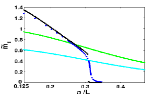
Figure 1: $\tilde{m}_{1}$ versus $\sigma$ for $g=0.5$, TL units and $\alpha=0$ (black) and $\alpha=0.1$ (blue). The cyan curve is for $0-1.5$ binary units and green for $0-2$ B units, both at $\alpha=0$.

$0-1$ binary networks fail to exhibit non-uniform retrieval (Fig.1; Ana05 and Kor05 ). The reason is simply related to setting the sparsity, and it can be understood intuitively as follows. There are two conditions to be satisfied for the retrieval state to exist: $m_{0}=\frac{1}{N}\int dr(\eta^{\mu}(r)/a-1)v(r)=O(1)$ and $x=\frac{1}{N}\int drv(r)=a$. The second means that, for spatially modulated retrieval states, in some parts of the network units with activity 1 in the corresponding stored pattern should have activity below 1, and in other parts above 1. The latter requirement poses no problem to the TL network, whose units can reach high levels of activity. For a network with binary units, or with units that saturate, the crucial issue is whether the up state, or the saturation level, is sufficiently above 1 (the arbitrarily set activity level of active units in the stored patterns; obviously the argument can be generalized to non-binary stored patterns). Thus binary units with activity levels, say, $0$ and $1.5$ (relative to the up state in the stored pattern) should be able to show spatially modulated activity profiles, although, rather than localized bumps, they appear as square-shaped spatially restricted activity. This results in the cyan and green curves for $\tilde{m}_{1}$ in Fig.1.

To further assess the effect of the saturation level on the formation of localized retrieval states we consider the following input-output function:

$$F(x)=\varepsilon\tanh(gx/\varepsilon)\Theta(x).$$

One should notice that $g$ is the slope at threshold and that for a sufficiently high $\varepsilon$ this is effectively just a TL function. For simplicity we focus on the $\alpha\to 0$ limit, as we do not expect the quenched noise to make any qualitative change in the behavior of the system, except for the smoothness of the transition. Fig.2 shows how $\tilde{m}_{1}$ changes with $\sigma$ for fixed $g=0.5$ and different values of saturation, as measured by $\varepsilon$. When the saturation is set at $\varepsilon=1$, for the intuitive reason above the first Fourier mode does not differ from zero. By increasing $\varepsilon$, however, one approaches the TL regime. In Fig.3 we plot $\tilde{m}_{1}$ versus $\sigma$ for different values of $g$ and both TL and saturating input-output functions. Notice the quasi-linear behavior for values of $\sigma$ below the transition.

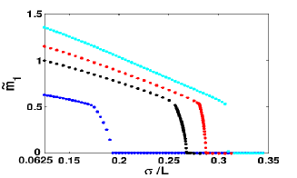
Figure 2: $\tilde{m}_{1}$ versus $\sigma$ for $g=0.5$ for different values of the saturation level: $\varepsilon=2$ (blue), $\varepsilon=3$ (black) and $\varepsilon=4$ (red). Cyan: TL units ($\varepsilon\to\infty$).

When $\alpha=0$, analyzing the formation of non-uniform solutions becomes simple even for a $d$-dimensional network. In this case, the fixed-point equations read:

$$\frac{\tilde{m}_{{i_{1}},\dots{i_{d}}}}{\tilde{\wp}_{{i_{1}},\dots{i_{d}}}} = \frac{1}{C}\int d\textbf{r}\prod^{d}_{n=1}c(i_{n}r_{n})<(\frac{\eta^{\mu}(\textbf{r})}{a}-1)F(h(\textbf{r},\eta^{\mu}))>$$

$$x = \frac{1}{N}\int d\textbf{r}<F(h(\textbf{r},\eta^{\mu}))>$$

$$h(\textbf{r},\eta^{\mu}) = (\frac{\eta^{\mu}(\textbf{r})}{a}-1)m(\textbf{r})-Th.$$ (10)

One can see that $m_{{i_{1}},{i_{2}},\dots{i_{d}}}=(1-a)\delta_{i_{1}0}\delta_{i_{2}0}\dots\delta_{i_{d}0}$ and $Th=(1-a)(1/a-1)-F^{-1}(1)$ solve the above equations, provided $F^{-1}(1)<(1-a)/a$ note1 . However, for the following connectivity probability distribution:

$$\wp(\textbf{r},\textbf{r}^{\prime})=\frac{c}{(2\pi\sigma^{2})^{\frac{d}{2}}}\prod^{d}_{i=1}exp(\frac{-(r_{i}-r^{\prime}_{i})^{2}}{2\pi\sigma^{2}})$$

this solution is stable only for $\sigma>\sigma_{c}$, where:

$$\sigma_{c}=\frac{L}{\pi}\sqrt{\frac{2}{d}\ln(a(1/a-1)^{2}F^{\prime}(F^{-1}(1)))}$$ (11)

and $L$ is the half length of each dimension. For $\sigma<\sigma_{c}$ the uniform solution becomes unstable in the direction of the first Fourier mode $\tilde{m}_{1\dots 1}$. In a network of TL units the equation for $\tilde{m}_{1\dots 1}$ – provided $\tilde{m}_{1\dots 1}<a/[g(1-a)]$ – reads $\tilde{m}_{1\dots 1}=g(\tilde{\wp}_{1\dots 1}/C)a(1/a-1)^{2}\tilde{m}_{1\dots 1}$, which at $\sigma_{c}$ is satisfied for any $\tilde{m}_{1\dots 1}$. This means that the system is marginally stable at this point in the direction of $\tilde{m}_{1\dots 1}$, resulting in a jump to $\tilde{m}_{1\dots 1}=a/[g(1-a)]$ for $\sigma<\sigma_{c}$, as shown in the graphs. It is worth noting that such trivial equation for $\tilde{m}_{1\dots 1}$ comes directly from the linear nature of the TL function above threshold. Adding quenched noise to a network of TL units or using any other function, e.g. the 2 introduced above, would change this trivial equation to a non-linear form, with the disappearance of the jump, as evident in figures Fig.1, 2, and 3.

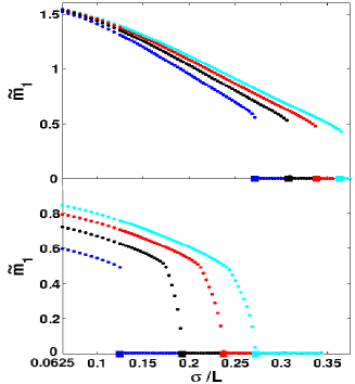
Figure 3: $\tilde{m}_{1}$ versus $\sigma$ for different values of the gain: $g=0.45$ blue, $g=0.5$ black, $g=0.55$ red and $g=0.6$ cyan. (upper panel) TL and (lower panel) saturating units with $\varepsilon=2$. With saturating units decreasing $g$ (thus linearizing the input-output function close to threshold) sharpens the transition. The filled squares represent $\sigma_{c}$ as predicted by Eq.11.

We further investigate the effect of localized retrieval on the storage capacity of the network. In Fig.4 we plot $\tilde{m}_{0}$ as a function of $\alpha$ for $\sigma=500$ and $800$. Even though the storage capacity ($\alpha_{c}={\rm Inf}_{\alpha}\{\alpha|\tilde{m}_{0}(\alpha)=0\}$) decreases, the decrease is not too severe, even for very localized solutions. Thus, the maximum number of retrievable patterns remains proportional to $C$.

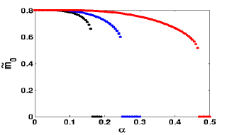
Figure 4: $\tilde{m}_{0}$ versus $\alpha$ for different values of $\sigma$ in a TL network with $g=0.5$. Black for $\sigma=500$, blue for $\sigma=800$ and red for structure-less network. Note the corresponding values: $\tilde{m}_{1}=1.22$ for $\sigma=500$, $\tilde{m}_{1}=0.8$ for $\sigma=800$ and $\tilde{m}_{1}=0$ for the structure-less network, all when $\alpha=0.05$.

The results presented here show that in general, a network with realistic single unit input-output transfer function becomes capable of localized retrieval simply by manipulating single unit saturation and linear gain. Increasing the gain, and/or the saturation level, makes retrieval states more localized. These parameters can be effectively controlled via inhibitory mechanisms. The effect of the quenched noise is minor on the qualitative behavior of the system, making the analytic formula Eq.11 a reasonable approximation for a wide range of parameters. The fact that for a given value of $\sigma$, changing the saturation level or the slope at threshold ($g$) can put the network out of the spatially modulated retrieval regime may explain the result of Ana05 .

Localized retrieval, while quantitatively decreasing local storage capacity, may considerably increase the computational power of a network with structured connectivity. This can be appreciated by noting that in a large network, more than one memory pattern of activity may be retrieved at the same time, each in a different location, without much interference. A combination of locally retrieved memories can be thought of as a global, composite memory pattern. The number of such composite patterns would be combinatorially large, thus hugely increasing the overall storage capacity of the network.

Moreover, while sparsity measures e.g. in IT cortex tend to yield high values (such as $a\simeq 0.7$ Rol98 ; Tre99 ) – seemingly in contradiction with the notion that associative networks require sparse coding in order to operate with a viable storage capacity – our result suggests another perspective. The reported values of $a$ may have been measured, effectively, conditional to the recorded units being active in a localized retrieval state, thus ‘overestimated’ by neglecting the large silent part of the network.

Each neuron in the neocortex receives of the order of $10^{4}$ synapses, and this number regulates a similar number of locally retrievable patterns. The fact that the number of memories stored in the neocortex seems much higher may stem from the combinatorial character of global memory patterns, allowed by the localization discussed here.

References

(1)
E. T. Rolls and A. Treves, Neural networks and brain function
(Oxford University Press: Oxford)(1998)
(2)
T. J. Will et al, Science, 308, 5723 (2005)
(3)
V. Braitenberg and A. Schuz, Anatomy of the Cortex (Springer:
Berlin) (1991)
(4)
Y. Roudi and A. Treves, JSTAT 1, P07010, (2004)
(5)
D. J. Amit, Modeling brain function (Cambridge University Press: Cambridge) (1989)
(6)
J. J. Torres et al, Neurocomputing 58, 229 (2004)
(7)
L. G. Morelli et al, Eur. Phys. J. B 38, 495 (2004)
(8)
A. Anishchenko et al, q-bio.NC/0502003
(9)
K. Koroutchev and E. Korutcheva, cond-mat/0503626
(10)
A. Treves et al, Neural Computation 11, 601 (1999)
(11)
M. Shiino and T. Fukai, J. Phys. A: Math. Gen. 25, L375 (1992)
(12)
This condition would impose some constraints on the parameters
that characterize the single unit input-output function. For
instance in the TL case it means , which in a
cortical network may be satisfied via inhibitory mechanisms.