Ring Exchange and Phase Separation in the two-dimensional Boson Hubbard model

Abstract

We present Quantum Monte Carlo simulations of the soft-core bosonic Hubbard model with a ring exchange term $K$. For values of $K$ which exceed roughly half the on-site repulsion $U$, the density is a non-monotonic function of the chemical potential, indicating that the system has a tendency to phase separate. This behavior is confirmed by an examination of the density-density structure factor at small momenta and real space images of the boson configurations. Adding a near-neighbor repulsion can compete with phase separation, but still does not give rise to a stable normal Bose liquid.

Introduction

The most commonly studied Hamiltonians of quantum spins and bosons include kinetic energy in the form of two site exchange. However, it was realized early on that, for lighter atoms, larger numbers of particles can permute their positions, leading to ring exchange terms.Thouless65 Interest in such models subsequently developed for a number of reasons, most recently as a result of the possibility of the existence of a normal bose liquid. Such a phase which might reconcile apparently contradictory observations in cuprate superconductors in the pseudogap regime where there is evidence of local pairing without superconductivity.Paramekanti02 ; Doniach03 Indeed, the magnitude of ring exchange terms in high-$T_{c}$ materials could be a significant fraction of the two site exchange.Coldea01 ; Katanin02 ; MullerHartmann02

Over the past several years, considerable numerical effort has been expended in looking at the low temperature phases of Hamiltonians including ring exchange.Melko04 ; Park02 ; Rousseau04 ; Roux05 Interestingly, while the normal bose liquid has remained somewhat elusive, a rich panoply of other behavior has been observed, including striped order, Neel antiferromagnetism, valence bond solids, and phase separation. The nature of the phase diagram and of the phase transitions between the different ordered phases remains an area of active inquiry.Sandvik05 Very recently it was proposedBuchler05 that ring exchange terms might be engineered into cold atomic gases, opening up the possibility that the effects of such terms could be studied in a situation where they can be tuned systematically, and hence the theoretical predictions checked experimentally.

In this paper we will extend our previous workRousseau04 on phase separation in the boson Hubbard model with ring exchange. We focus on two dimensions, since that is the lowest dimension allowing ring exchange processes, and it is the effective dimension of the CuO₂ sheets of the cuprate superconductors which have motivated much of the recent study of Bose liquid phases. Our key conclusion is that when the ring exchange energy scale exceeds approximately one half the on-site repulsion, the ground state is thermodynamically unstable to phase separation. Adding a near-neighbor repulsion can prevent phase separation, but the ground state always has either nonzero checkerboard or superfluid order. Because we use a break-up of the Hamiltonian in constructing the path integral which has not been much employed before, we also describe some of the technical details of the simulation, including the effectiveness of different local Quantum Monte Carlo (QMC) moves.

The most simple boson Hubbard modelFisher89 is:

$$\hat{\mathcal{H}}=-t\sum_{\bigl{\langle}ij\bigr{\rangle}}(a_{j}^{\dagger}a_{i}+a_{i}^{\dagger}a_{j})+U\sum_{i}\hat{n}_{i}(\hat{n}_{i}-1)$$ (1)

The operators $a_{j}^{\dagger},a_{j}$ create (destroy) a boson on site $j$, and obey commutation rules $\bigl{[}a_{i},a_{j}^{\dagger}\bigr{]}=\delta_{ij}$. The number operator is $\hat{n}_{j}=a_{j}^{\dagger}a_{j}$. The hopping parameter $t$ measures the kinetic energy and $U$ the strength of the on-site repulsion. The sum $\langle ij\rangle$ is over near neighbors on a square lattice. In the limit $U\rightarrow\infty$ this model maps onto the spin-1/2 XY model, with the magnetization playing the role of the bosonic density. By now, the $T=0$ phase diagram of the boson Hubbard Hamiltonian is well known.Fisher89 ; Batrouni90 ; Kuhner00 ; Freericks96 ; Krauth91 ; vanOtterlo94 ; Prokofev04 Away from commensurate filling, the ground state is superfluid. At commensurate fillings, and for sufficiently large $U$, a Mott insulator forms in which each site is occupied by an integer number of particles.

Our goal is to consider the effect of a ring exchange term:

$$\hat{\mathcal{K}}=-K\sum_{\left\{p\right\}}(a_{1}a_{2}^{\dagger}a_{3}^{\dagger}a_{4}+a_{1}^{\dagger}a_{2}a_{3}a_{4}^{\dagger})$$ (2)

The ring exchange term acts on four site plaquettes $\bigl{\{}p\bigr{\}}$, destroying two particles which lie along one diagonal, and creating them on the other. Because of the minus sign in (2), the energy decreases when the particles are exchanged. The basic qualitative picture behind the suggestion that the ring exchange term might give rise to a normal Bose liquid is that if one starts with a superfluid phase, $K$ introduces local vortices in which two particles jump in opposite directions. These local twists, if sufficiently favored energetically, could compete with, and ultimately prevent, a coherent long range superflow of particles. At the same time, such a hopping process increases (local) quantum fluctuations, and would not be expected to make the system incompressible (a Mott insulator). Therefore one might have a normal Bose liquid.

As we shall see, we find that this ring exchange term causes phase separation rather than a normal Bose liquid. It is natural to attempt to resurrect the liquid by adding a longer range repulsion which acts against particle clustering. The most simple form is a near-neighbor repulsion:

$$\hat{\mathcal{V}}=V\sum_{\bigl{\langle}ij\bigr{\rangle}}\hat{n}_{i}\hat{n}_{j}$$ (3)

The effects of near neighbor repulsion in the absence of ring exchange have been well-studied in the context of the boson Hubbard Hamiltonian.Niyaz93 They are perhaps most simply ascertained by considering the hard-core limit and the equivalent spin model. As commented earlier, the boson kinetic energy corresponds to an $XY$ spin coupling. $V$ corresponds to a $Z$ coupling. Thus when $V<2t$ the spin model is in the $XY$ universality class (a boson superfluid) and for $V>2t$ the spin model is in the Ising universality class (a checkerboard charge density boson insulator). A considerable amount of work has also been done on looking for supersolid phases which combine superfluid and charge density wave (CDW) order.OtherSS ; Batrouni00

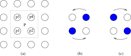
Figure 1: The ring exchange term acts on each square plaquette of our 2d lattice (a), and allows the exchange of two particles from one diagonal (b) to the other (c).

QMC: The Partition Function as a Path Integral

Our Quantum Monte Carlo simulations are performed using a World Line algorithm with a decomposition involving four site matrix elements. We discuss the algorithm in detail here because this decomposition, which is similar but not identical to reference Loh85 , is used considerably less frequently than the more conventional approach which involves two site matrix elements.twositedecoupling In fact, to our knowledge, it has not been employed before for Hamiltonians including ring exchange, although stochastic series expansion approachesSandvik91 are formally very similar. A specific issue we will address is the effect of different local moves on the measurement of the energy.

We begin by representing the partition function as a path integral, in which $e^{-\beta\hat{\mathcal{H}}}$ is the imaginary time evolution operator, $0\leq\tau\leq\beta$. The goal is to take the exponential of the full Hamiltonian, which cannot be computed, and express it in terms of exponentials whose numerical values can be written down. In order to accomplish this, we write the full imaginary time evolution operator as a product of infinitesimal evolution operators over short imaginary times $\Delta\tau$:

$$\mathcal{Z}=\textrm{Tr }e^{-\beta\hat{\mathcal{H}}}=\textrm{Tr }(e^{-\Delta\tau\hat{\mathcal{H}}})^{M}\hskip 28.45274pt\tau=\frac{\beta}{M}$$ (4)

Here $M$ is chosen to be a sufficiently large integer so as to make $(\Delta\tau)^{2}$ times any two of the energy scales in $\hat{\mathcal{H}}$ small, as discussed further below.

We then divide the sum over all plaquette operators into four classes depicted by the different shadings (colors on-line) in Fig. 3. That is, the full Hamiltonian is written as

$$\hat{\mathcal{H}}=\hat{\mathcal{H}}_{1}+\hat{\mathcal{H}}_{2}+\hat{\mathcal{H}}_{3}+\hat{\mathcal{H}}_{4}$$ (5)

where

$$\hat{\mathcal{H}}_{n}=\sum_{p\in n}\hat{\mathcal{H}}_{p}$$ (6)

groups together all plaquettes of a given shading. In order to avoid overcounting the kinetic energy, on-site, and near neighbor interaction terms in the Hamiltonian we define,

$$\hat{\mathcal{H}}_{p}=\hat{\mathcal{K}}_{p}+\frac{1}{2}(\hat{\mathcal{T}}_{p}+\hat{\mathcal{V}}_{p})+\frac{1}{4}\hat{\mathcal{U}}_{p}$$ (7)

with

$$\hat{\mathcal{T}}_{p}=-t(a_{p1}^{\dagger}a_{p2}+a_{p3}^{\dagger}a_{p4}+a_{p1}^{\dagger}a_{p3}+a_{p2}^{\dagger}a_{p4}+h.c.)$$

$$\hat{\mathcal{K}}_{p}=-K(a_{p1}a_{p2}^{\dagger}a_{p3}^{\dagger}a_{p4}+h.c.)$$

$$\hat{\mathcal{U}}_{p}=U[\hat{n}_{p1}(\hat{n}_{p1}-1)+\hat{n}_{p2}(\hat{n}_{p2}-1)$$

$$\hskip 12.80365pt+\hat{n}_{p3}(\hat{n}_{p3}-1)+\hat{n}_{p4}(\hat{n}_{p4}-1)]$$

$$\hat{\mathcal{V}}_{p}=V(\hat{n}_{p1}\hat{n}_{p2}+\hat{n}_{p3}\hat{n}_{p4}+\hat{n}_{p1}\hat{n}_{p3}+\hat{n}_{p2}\hat{n}_{p4}).$$ (8)

It is important to emphasize that while plaquette operators acting on neighboring plaquettes do not commute, all plaqette operators within the same shading do commute, since they do not “touch.” This independence will enable us to compute their exponentials.

Figure 2: The application of $e^{-\Delta\tau\hat{\mathcal{H}}}$ propagates the boson occupations on the four spatial sites of the plaquette (a) in the imaginary time direction, and can be thought of geometrically as converting each spatial plaquette into a cube (b) whose bottom face contains the boson occupations before the action of the operator, and whose top face contains the boson occupations after the action of the operator.

Now we express each infinitesimal evolution operator as a product:

$$e^{-\Delta\tau\hat{\mathcal{H}}}=e^{-\Delta\tau(\hat{\mathcal{H}}_{1}+\hat{\mathcal{H}}_{2}+\hat{\mathcal{H}}_{3}+\hat{\mathcal{H}}_{4})}$$

$$\approx e^{-\Delta\tau\hat{\mathcal{H}}_{1}}e^{-\Delta\tau\hat{\mathcal{H}}_{2}}e^{-\Delta\tau\hat{\mathcal{H}}_{3}}e^{-\Delta\tau\hat{\mathcal{H}}_{4}}$$ (9)

Substituting expression (QMC: The Partition Function as a Path Integral) in expression (4), we get:

$$\mathcal{Z}=\textrm{Tr}(e^{-\Delta\tau\hat{\mathcal{H}}_{4}}e^{-\Delta\tau\hat{\mathcal{H}}_{3}}e^{-\Delta\tau\hat{\mathcal{H}}_{2}}e^{-\Delta\tau\hat{\mathcal{H}}_{1}})^{M}$$ (10)

The errors made in breaking up $e^{-\Delta\tau\hat{\mathcal{H}}}$, Eq. QMC: The Partition Function as a Path Integral, go as the commutator of the individual pieces, and therefore as $(\Delta\tau)^{2}$. It might be thought that the accumulation of the $(\Delta\tau)^{2}$ errors across the $M$ imaginary time slices might lead to an error linear in $\Delta\tau$. However, the expectation value of any Hermitian operatorFye86 ; Fye87 has a Trotter error which is quadratic in $\Delta\tau$.

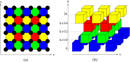
Figure 3: (a) Plaquettes with same shading (color online) are independent. (b) Introducing a dimension in imaginary time makes the plaquettes become cubes, each representing an infinitesimal evolution operator. Cubes with same shading don’t touch each other, while cubes with different shading act at different times and therefore are decoupled.

To complete the evaluation of the trace, we work in the basis of occupation numbers $\left|\left\{n\right\}\right\rangle$. Inserting a complete set of states $I=\sum_{\left\{n\right\}}\left|\left\{n\right\}\right\rangle\left\langle\{n\}\right|$ between each pair of exponentials, we get:

$$\begin{array}[]{ll}\mathcal{Z}=\displaystyle\sum_{\left\{n^{k}\right\}}&\displaystyle{\prod_{k=1}^{M}}\left\langle\left\{n^{k+1}\right\}\right|e^{-\Delta\tau\hat{\mathcal{H}}_{4}}\bigl{|}\bigl{\{}n^{k+3/4}\bigr{\}}\bigr{\rangle}\\ &\times\left\langle\left\{n^{k+3/4}\right\}\right|e^{-\Delta\tau\hat{\mathcal{H}}_{3}}\left|\left\{n^{k+1/2}\right\}\right\rangle\\ &\times\left\langle\left\{n^{k+1/2}\right\}\right|e^{-\Delta\tau\hat{\mathcal{H}}_{2}}\left|\left\{n^{k+1/4}\right\}\right\rangle\\ &\times\left\langle\left\{n^{k+1/4}\right\}\right|e^{-\Delta\tau\hat{\mathcal{H}}_{1}}\left|\left\{n^{k}\right\}\right\rangle\end{array}$$ (11)

The superscripts $k$ appearing in the sets $\left\{n^{k}\right\}$ label the imaginary time, emphasizing that a different complete set of states has been introduced between each pair of exponentials. Since operators acting on plaquettes with the same shading commute, each matrix element in (11) can be written as a product of four site matrix elements

$$\!\bigl{\langle}\bigl{\{}n^{q+1/4}\bigr{\}}\bigr{|}e^{-\Delta\tau\hat{\mathcal{H}}_{n}}\left|\left\{n^{q}\right\}\right\rangle\!=\!\!\prod_{p(q)}\!\bigl{\langle}\mathcal{P}^{q+1/4}\bigr{|}e^{-\Delta\tau\hat{\mathcal{H}}_{p}}\left|\mathcal{P}^{q}\right\rangle$$ (12)

where $\mathcal{P}^{q}$ represents the state at imaginary time $q$ ($q$ is a multiple of $\frac{1}{4}$) of the four sites belonging to plaquette $p$, and $\prod_{p(q)}$ is a product over all matrix elements between times $q$ and $q+1/4$. The entire evolution is represented by an interconnected set of the cubes of Fig. 2b, as illustrated in Fig. 3b.

Since each $\hat{\mathcal{H}}_{p}$ conserves the sum of the boson numbers on the four spatial sites, the occupation numbers living on these cubes trace out continous ‘world-lines’ of particles which wiggle and deform during their evolution. Furthermore, because we are evaluating the trace of $e^{-\beta\hat{\mathcal{H}}}$, the occupation numbers and associated world lines are periodic in imaginary time. We will discuss the sampling of the expression for $\mathcal{Z}$, and the associated conservation laws, in more detail below.

Summarizing, the partition function takes the simple form of a sum of products of four site matrix elements,

$$\mathcal{Z}=\sum_{\left\{\mathcal{P}^{k}\right\}}\prod_{k=1}^{M}\prod_{p(k)}\bigl{\langle}\mathcal{P}^{k+1/4}\bigr{|}e^{-\Delta\tau\hat{\mathcal{H}}_{p}}\left|\mathcal{P}^{k}\right\rangle$$ (13)

The imaginary time index $k$ runs from $1$ to $M$ with step $\frac{1}{4}$. Each matrix element in (13) can be computed by numerical diagonalization if we assume that occupation numbers are never greater than four. (This restriction is satisfied in all simulations here, since the average densities studied are of order unity.highocc ) Each site has five possible states and the number of different states for one plaquette is $5^{4}=625$. To compute the exponential of $\hat{\mathcal{H}}_{p}$ then requires the diagonalization of a $625\times 625$ matrix.

Sampling of the partition function

In order to perform measurements, one needs to generate sets of world lines with the Boltzmann weight given by the summand of Eq. 13. This is done using a Metropolis algorithm. One starts with straight world lines, then suggests local deformations and accepts them with probability $p=\textrm{min}(1,{\cal R})$, where ${\cal R}$ is the ratio of the Boltzmann weight after the move to that before. In the usual way, this satisfies detailed balance. To ensure ergodicity of the algorithm, different kinds of moves have to be included, like pull moves (Fig. 4a), “baby” pull moves (Fig. 4b), twist moves (Fig. 4c), and “baby” twist moves (Fig. 4d). Only a few of the plaquette matrix elements change when one of these local moves is performed. The most complex is the twist move (Fig. 4c) which involves 10 matrix elements (only 5 cubes are shown in order to make the figure clearer).

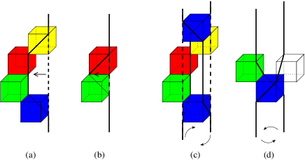
Figure 4: To ensure ergodicity of the algorithm, four kinds of moves must be included: (a) pull moves, (b) “baby” pulls, (c) twist moves and (d) “baby” twist moves.

These different kinds of moves are required in order to make the algorithm ergodic. As an illustration, we show in Fig. 5 the energy per particle of free bosons as a function of the inverse temperature $\beta$, with various types of moves suppressed. We can see that the correct energy $E(\beta)$ is obtained only when both pull and “baby” pull moves are included.

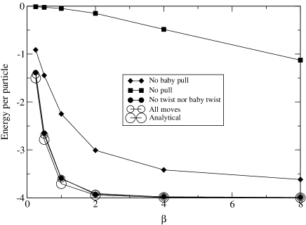
Figure 5: Energy per particle for free bosons as a function of the inverse temperature $\beta$ with and without including pull and baby pull moves.

It is notable in Fig. 5 that the correct energy is obtained even without the twist moves. It might be thought that this is because $K=U=0$ and that twist moves will become important when turning on interactions, especially with ring exchange processes. However this is not the case, as can be seen in Fig. 6. We believe this to be an advantage of the four site decomposition over the two site one. The four site decomposition already analytically includes twists in the evaluation of the matrix elements of the exponentials of the $H_{n}$.

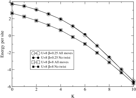
Figure 6: Energy per particle for interacting bosons as a function of the ring exchange strength $K$ with and without including twist moves.

While including only pull and “baby” pull moves seems to get the energy right on the lattice sizes studied above, our simulations are done with all moves included. These local moves all take the form of local distortions of existing world-lines and hence cannot change $\rho$. Thus our code works in the canonical ensemble. It simulates whatever value of $\rho$ with which we initialize the lattice. If desired, we can make contact with the grand-canonical ensemble, by computing the chemical potential as the energy cost, in the ground state, of adding a boson to the system, $\mu(N_{b})=E(N_{b}+1)-E(N_{b})$. Actually, canonical simulations have certain advantages in exploring phase separation, as we shall see, and as has previously been described.Batrouni00

Our simulations also are confined to the zero-winding sector of the space of all possible paths. This has implications for how we measure the superfluid density $\rho_{s}$. Consider the well-known relation,Pollock87

$$\rho_{s}=\frac{\bigl{\langle}\hat{W}^{2}\bigr{\rangle}}{2dt\beta}$$ (14)

where $d$ is the dimension of the system, and $\bigl{\langle}\hat{W}^{2}\bigr{\rangle}$ the mean square of the winding number operator which measures the net flow of particles off the right side of the lattice and over to the left side. Our local moves cannot change the winding, as is evident by comparing the configurations of Fig. 7. Hence, using Eq. (14) our algorithm would systematically give a zero value for the superfluid density, if we begin in a $W=0$ configuration.

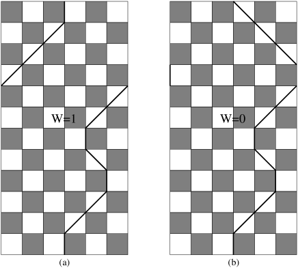
Figure 7: Example of world line with $W=1$ (a) and $W=0$ (b) winding numbers in the case of a one dimensional lattice. Configurations with non-zero winding number cannot be reached with local moves.

However, we can still measure $\rho_{s}$. The procedure is as follows: We define the pseudo-current operator (using the notation of Fig. 2b for the site labels)

$$\begin{array}[]{l}\displaystyle\hat{j}_{x}(k)=\sum_{c\in(k,k+1)}\left(\hat{n}_{c6}+\hat{n}_{c8}-\hat{n}_{c2}-\hat{n}_{c4}\right)\\ \displaystyle\hat{j}_{y}(k)=\sum_{c\in(k,k+1)}\left(\hat{n}_{c7}+\hat{n}_{c8}-\hat{n}_{c3}-\hat{n}_{c4}\right)\end{array}$$ (15)

where the sum $\sum_{c\in(k,k+1)}$ is over all cubes of Fig. 3b between times $k$ and $k+1$. These quantities measure the number of particles which jump in the positive $x$ and $y$ directions between imaginary times $k$ and $k+1$. The winding number operators in both $x$ and $y$ directions are then given by

$$\begin{array}[]{l}\displaystyle\hat{W}_{x}=\frac{1}{N_{x}}\sum_{k=1}^{M}\hat{j}_{x}(k)\\ \displaystyle\hat{W}_{y}=\frac{1}{N_{y}}\sum_{k=1}^{M}\hat{j}_{y}(k)\end{array}$$ (16)

where $N_{x}$ and $N_{y}$ are respectively the number of sites in the $x$ and $y$ directions. We measure also the auto-correlation function of the pseudo-current:

$$\begin{array}[]{l}\displaystyle\mathcal{J}_{x}(k)=\sum_{k^{\prime}}\left\langle\hat{j}_{x}(k+k^{\prime})\hat{j}_{x}(k^{\prime})\right\rangle\\ \displaystyle\mathcal{J}_{y}(k)=\sum_{k^{\prime}}\left\langle\hat{j}_{y}(k+k^{\prime})\hat{j}_{y}(k^{\prime})\right\rangle\end{array}$$ (17)

and compute its Fourier transform via

$$\widetilde{\mathcal{J}_{x,y}}(\omega_{n})=\sum_{k}\mathcal{J}_{x,y}(k)e^{i\omega_{n}k}$$ (18)

where $\omega_{n}=\frac{2\pi}{M}n$.

One can show that these pseudocurrent operators are related to the winding by,

$$\begin{array}[]{l}\displaystyle\bigl{\langle}\hat{W}_{x}^{2}\bigr{\rangle}=\frac{\widetilde{\mathcal{J}_{x}}(0)}{N_{x}^{2}}\\ \displaystyle\bigl{\langle}\hat{W}_{y}^{2}\bigr{\rangle}=\frac{\widetilde{\mathcal{J}_{y}}(0)}{N_{y}^{2}}\end{array}$$ (19)

As already stated, the measurement of the winding number, and hence the Fourier transform at $\omega_{n}=0$, will give a zero value. but we can avoid the problem by considering the finite frequency response. In fact, one can showBatrouni90 that the correct, nonzero, winding number and $\rho_{s}$ are given by taking the zero frequency limit of $\widetilde{\mathcal{J}_{x}}(\omega_{n})$, as illustrated in Fig. 8.

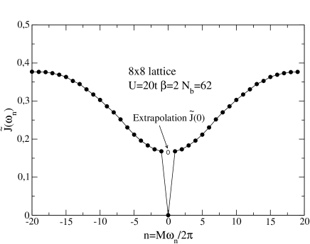
Figure 8: Restricting the winding number to a zero value introduces a discontinuity in the Fourier transform of the pseudo-current auto-correlation function. Performing an extrapolation gives the correct value of the superfluid density.

Results: Hard-core limit, $V=0$

We can work in the hard-core limit by running a soft-core code at large $U$, or more directly by forbidding the acceptance of multiple occupancies in our Monte Carlo moves. This also simplifies the computation of the matrix elements in (13) since we can restrict to single occupancy states (and hence diagonalize only a $16\times 16$ matrix). Such a hard-core model is equivalent to replacing the standard bosonic commutation rules by the hard-core rules,

$$\begin{array}[]{lll}\left\{a_{i},a_{i}\right\}=0&\left[a_{i},a_{j}\right]=0&\forall i\neq j\\ \bigl{\{}a_{i}^{\dagger},a_{i}^{\dagger}\bigr{\}}=0&\bigl{[}a_{i}^{\dagger},a_{j}^{\dagger}\bigr{]}=0&\forall i\neq j\\ \bigl{\{}a_{i},a_{i}^{\dagger}\bigr{\}}=1&\bigl{[}a_{i},a_{j}^{\dagger}\bigr{]}=0&\forall i\neq j\,,\end{array}$$ (20)

where $\bigl{\{}A,B\bigr{\}}=AB+BA$ is an anti-commutator. The usual bosonic commutators between operators acting on different sites ensure that the wave function is symmetric in the exchange of particles, as required for bosons.

Our simulations are done mainly on $16\times 16$ lattices. We always take $t=1$ for the hopping parameter, which thereby sets the energy scale. We will also set the near neighbor interaction $V=0$ until the final results section.

In order to describe the different phases of the system, in addition to the superfluid density $\rho_{s}$, we measure the Fourier transforms of the density-density and plaquette-plaquette order correlation functions, $S(\pi,\pi)$, $P(\pi,0)$ and $P(0,\pi)$ defined by,

$$S\bigl{(}k_{x},k_{y}\bigr{)}=\frac{1}{\bigl{(}N_{x}N_{y}\bigr{)}^{2}}\sum_{\vec{r},\vec{r}^{\>\prime}}\bigl{\langle}\hat{n}_{\vec{r}}\,\,\hat{n}_{\vec{r}+\vec{r}^{\>\prime}}\bigr{\rangle}e^{-i\vec{k}\cdot\vec{r}}$$ (21)

$$P\bigl{(}k_{x},k_{y}\bigr{)}=\frac{1}{K^{2}\bigl{(}N_{x}N_{y}\bigr{)}^{2}}\sum_{p,p^{\prime}}\bigl{\langle}\hat{\mathcal{K}}_{p}\hat{\mathcal{K}}_{p^{\prime}}\bigr{\rangle}e^{-i\vec{k}\cdot(\vec{r}_{p}-\vec{r}_{p^{\prime}})}$$ (22)

Fig. 9 shows these quantities, and the superfluid density, as a function of $K$ at half filling. Increasing $K$ makes the superfluid density decrease. $\rho_{s}$ vanishes completely around $K=8$. At the same time, the plaquette structure factors $P(\pi,0)$ and $P(0,\pi)$ start to grow, indicating the formation of stripes by the ring exchange. This is the VBS (Valence Bond Solid) phase, previously discussed in quantum spin systems. Stripe formation is also observable by considering the correlations in the hopping from plaquette to plaquette, rather than the ring exchange. For higher values of $K$, the VBS phase becomes unstable and is replaced by a CDW as shown by the growth of $S(\pi,\pi)$.Melko04

Both the VBS and CDW phases are gapped. That is, the energy needed to add a particle to the lattice (the chemical potential) jumps abruptly across $\rho=\frac{1}{2}$. We define $G=\mu_{+}-\mu_{-}$ with $\mu_{+}=E\bigl{(}N_{b}={N\over 2}+1\bigr{)}-E\bigl{(}{N\over 2}\bigr{)}$ and $\mu_{-}=E\bigl{(}{N\over 2})-E\bigl{(}{N\over 2}-1\bigr{)}$. $G=0$ in the superfluid phase $K<8$, and is non-zero for $K>8$. The VBS and CDW phases are insulators. Fig. 10 shows $G$ as one increases $K$ out of the superfluid phase at half-filling.

Figure 9: The superfluid density and the order parameters for the hard-core case at half filling for a $16\times 16$ lattice. Increasing $K$ destroys the superfluid density. Then a solid order appears corresponding to a VBS phase. This phase becomes unstable if increasing $K$ more, and yields to a CDW phase.

Figure 10: The gap in the chemical potential at half filling, as a function of $K$ for a $16\times 16$ Lattice. The gap starts to appear at $K\simeq 8$, coincident with the vanishing of $\rho_{s}$, and grows as $K$ is increased, showing the presence of insulating phases.

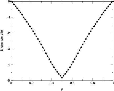
Figure 11: The energy per site as a function of the density $\rho$, for $K=10$ on a $8\times 8$ Lattice.

We now consider what happens when the system is away from half-filling. Fig. 11 shows the energy as a function of density. There are several interesting features. First, the kink in the energy right at half-filling is associated with a nonzero gap. Second, there is a region of densities for which the energy is concave down. As a consequence, the usual Maxwell construction indicates that it is energetically more favorable to have two separate regions of different density than a single region of uniform density. The system phase separates.

Figure 12: The density of particles as a function of the chemical potential, for $K=10$ ($8\times 8$ Lattice).

The energetic signature of phase separation is further illustrated in Fig. 12, which shows the density of particles $\rho$ as a function of the chemical potential $\mu$ over a wide range of densities. The jump of the chemical potential at half filling is the gap associated with the solid VBS phase discussed above. The regions where the slope of the curve (proportional to the compressibility $\kappa_{T}$) is negative indicate that the system is thermodynamically unstable Batrouni00 and undergoes phase separation. There are two such regions. The first is seen as soon as we go away from half filling, ie for the two fillings $N/2\pm 1$ immediately adjacent to half-filling, and indicates a first order transition from the VBS phase to a superfluid. (See also Fig. 14.) The same negative compressibility near half-filling is obtained for values of $K$ higher than 15, showing a first order transition from the CDW phase to a superfluid. The second region of negative compressibility occurs below $\rho_{c}=0.34$.

The spikes occuring at $\rho\approx 0.1$ and $\rho\approx 0.2$ in Fig. 12 are not due to statistical fluctuations. Indeed, when phase separating, the system can form a stripe in its density profile rather than an island, due to periodic boundary conditions. This produces a shift in the energy, and hence in the chemical potential. In our simulations, the system forms a stripe for $\rho\in[0.1,0.2]$, and an island when crossing the limits, generating the spikes.

While analysis of the energy and chemical potential yield quantitative information about the regions of stability, a more straightforward, qualitative, indication of clustering comes from simple real space images of the boson density during the course of a simulation. Whether clustering occurs or not, if the density is averaged over the whole simulation, we should observe a uniform density distribution, since the probability of a state is independant of any translation in the lattice. But if the density is averaged over only a few iterations, we observe a density profile reflecting the clustering (Fig. 13).

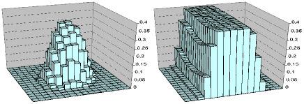
Figure 13: Typical QMC results for the average density distribution when the clustering occurs. For a density $\rho=12/256$ the system adopts a shape of an island, while for $\rho=48/256$ the system prefers to form a stripe, which, in the presence of periodic boudary conditions, is the geometry which maximizes the number of occupied four site plaquettes for which the ring exchange energy is low.

To corroborate further that this negative compressibility is associated with phase separation, we define the observable $\Omega$ to be the average of the density structure factor over the smallest values of the wave vector:

$$\Omega=\frac{S(\epsilon_{x},0)+S(\epsilon_{x},\epsilon_{y})+S(0,\epsilon_{y})}{3}\hskip 14.22636pt\epsilon_{x,y}=\frac{2\pi}{N_{x,y}}$$ (23)

$\Omega$ measures modulations of the density profile with wave lengths on the order of the size of the lattice. Fig. 14 shows the superfluid density and $\Omega$ as functions of the density of particles $\rho$, for a fixed value $K=10$. The symmetry of the curves reflects the particle-hole symmetry of the hard-core Hamiltonian. Starting from $\rho=\frac{1}{2}$ where $\Omega$ and $\rho_{s}$ have a zero value, and which corresponds to the VBS phase, we see that doping the system increases the superfluid density rapidly. $\rho_{s}$ reaches its maximum for $\rho\simeq 0.4$ (or $\rho\simeq 0.6$ by symmetry). Then $\rho_{s}$ falls at the same time that $\Omega$ grows and reaches its maximum for $\rho\simeq 0.2$ (or $\rho\simeq 0.8$). Fig. 14 suggests that as soon as we go away from half-filling, there is a transition from the VBS phase first to a stable superfluid, but that subsequently phase separation sets in. The density $\rho\simeq 0.3$ where $\rho_{s}$ falls and $\Omega$ increases rapidly matches quite well with the density at which $\kappa$ changes sign in Fig. 12.

Figure 14: Superfluid density and $\Omega$ as functions of the density of particles, for $K=10$ on an $8\times 8$ Lattice.

The occurrence of phase separation indicated in the compressibility, $\Omega$, and in real space images, may be understood with a simple physical picture. When $K$ is sufficiently large, the system increases the ring exchange processes in order to decrease its energy. But ring exchange is possible only if there are second neighbor particles. Thus in a dilute collection of particles, the ring exchange term has a tendency to act as an attractive potential. This is not true of the usual kinetic energy, since there a single boson can hop by itself without needing a partner.

One can analyze this binding quantitatively for the case of two bosons by exact diagonalization (Lanczos). Fig. 15 shows the square root of the mean quadratic distance $\bigl{\langle}\hat{r}^{2}\bigr{\rangle}$ between two particles for different $L\times L$ lattice sizes in the ground state. The soft-core case is considered with an on-site repulsion $U=12t$. For low values of $K$ the distance between the bosons grows linearly with $L$, as one would expect if the particles were distributed independently across the lattice. On the other hand, for high values of $K$, the distance between the particles is relatively independent of lattice size, suggesting the particles stay together, and demonstrating the existence of a bound state. While the data shown are for $U=12t$, the phenomenon is independent of $U$, and, in particular, is seen also in the hard-core case. The reason the on-site repulsion $U$ does not successfully compete with the binding is that the bound wavefunction favors the bosons on second-near-neighbor sites where $U$ plays no role. This is reflected in the data of Fig. 15 where we see that the distance between the paired bosons is still several lattice sites.

Figure 15: The mean square distance $\sqrt{\bigl{\langle}\hat{r}^{2}\bigr{\rangle}}$ between two particles as a function of $K/t$, in the soft-core case with $U=12t$ at $T=0$.

Figs. 12 and 14 showed our results for hard-core bosons at fixed $K=10$ as the system is doped. By performing further simulations for different values of $K$, we are able to generate the complete phase diagram of hard-core bosons (Fig. 16) in the $K-\rho$ plane. Gapped VBS and CDW phases exist only at half-filling and relatively large $K$. For weaker $K$ and half-filling the system is superfluid. When the system is doped a small amount away from half-filling, only a superfluid phase is present. Upon further doping, the clustering region is reached. As $K$ becomes large, clustering occurs closer and closer to half-filling.

Melko et al. Melko04 have studied the spin-1/2 Hamiltonian,

$$\hat{\mathcal{H}}=-J\sum_{\bigl{\langle}ij\bigr{\rangle}}\hat{\mathcal{B}}_{ij}-K\sum_{\bigl{\langle}ijkl\bigr{\rangle}}\hat{\mathcal{P}}_{ijkl}-h\sum_{i}\hat{\mathcal{S}}_{i}^{z}$$ (24)

where

$$\begin{array}[]{ll}\hat{\mathcal{B}}_{ij}=2\bigl{(}S_{i}^{x}S_{j}^{x}+S_{i}^{y}S_{j}^{y}\bigr{)}\\ \hat{\mathcal{P}}_{ijkl}=S_{i}^{+}S_{j}^{-}S_{k}^{+}S_{l}^{-}+S_{i}^{-}S_{j}^{+}S_{k}^{-}S_{l}^{+}\end{array}$$ (25)

and $S^{x}$, $S^{y}$, $S^{z}$, $S^{+}$, $S^{-}$ are the usual spin operators. This is the Heisenberg $XY$ model with a four spin exchange term and in a magnetic field. This model is exactly equivalent to our bosonic model in the hard-core limit. The magnetic field plays the role of the chemical potential in the grand canonical ensemble. In the phase diagram obtained by Melko et al., the superfluid, VBS and CDW phases are present and their boundaries match with our results. In addition the nature of the transitions also agree. Our simulations in the canonical ensemble exhibit clear phase separation indicating first order transitions from CDW insulator (Néel) to SF and also from SF to Mott (fully polarized, in the spin language). To see this, consider the phase diagram, Fig. 1 in Ref. [7]. As discussed in that paper, the cuts along lines $A$ and $B$ show clear hysteresis indicating first order transitions. Our simulations in Fig. 12 are done at constant $K$ and would correspond most closely to a vertical cut, like $A$, in Ref. [7] but going from Néel to SF to fully polarized. This way two first order phase transitions would be crossed, as shown in Fig. 12 here by the negative compressibility regions. Note also that the jump in the density when going from Néel to SF (e.g. cut $B$ in [7]) is very small as shown in the magnetization histogram, Fig. 3 of [7]. Recalling that $\rho=m+0.5$, we see that the jump in $\rho$ in the histogram is about $0.015$, of the same order as we see in our Fig. 12.

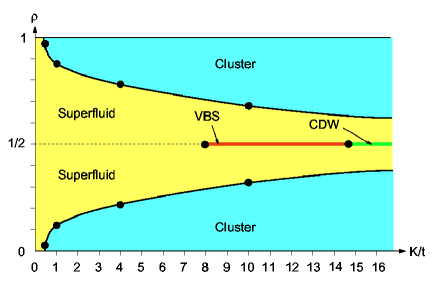
Figure 16: The phase diagram of hard-core bosons ($16\times 16$ Lattice). The solid phases (VBS and CDW) exist only at half-filling. When doping the system, the phase first becomes superfluid, then the clustering occurs closer to $\rho=\frac{1}{2}$ as $K$ is increased.

Thus, the hard-core bosonic model with ring exchange does not exhibit any compressible but non-superfluid, Bose-liquid, phase. In the next section we examine the possibilityParamekanti02 that the relaxation of the hard-core constraint could make the solid phases (VBS or CDW) evolve to a Bose liquid.

Results: Soft-core case, $V=0$

We now turn to the soft-core case, but still choose the intersite repulsion $V=0$ and half-filling. The superfluid density $\rho_{s}$ is shown as a function of $K$ for $U=8t$ in Fig. 17. $\rho_{s}$ first grows slightly when $K$ increases. When $K\simeq 4t$, $\rho_{s}$ starts to decrease. This decrease becomes rather rapid until, at $K\simeq 8t$, $\rho_{s}$ levels off at about half its $K=0$ value. This behavior is quite different from the hard-core case (inset) where $\rho_{s}$ decreases as soon as the ring exchange interaction is turned on, and vanishes at $K\simeq 8t$.

Figure 17: The superfluid density as a function of $K$ for the soft-core case where $U=8t$, at half-filling ($16\times 16$ Lattice). $\rho_{s}$ does not vanish when $K$ is large, unlike the hard-core case.

In order to understand the difference in the behavior of $\rho_{s}$ between the soft and hard core cases, we begin by examining $\Omega$, the small momentum density-density structure factor. Fig. 18 shows $\Omega$ as a function of $K$ for $U=4t$ and $U=8t$. In both cases, when $K$ reaches a value of the order $U/2$, $\Omega$ grows sharply, showing, as in the hard-core case, the presence of a clustering tendency. Results for $16\times 16$ and $24\times 24$ lattices are almost identical, indicating that the phase separation is not a finite size effect.

The behavior of the superfluid density can then be explained as follows: When $K$ is weak, the ring exchange term supports the motion of the particles, and helps the kinetic term in delocalizing them. A flow can thus occur more easily and $\rho_{s}$ increases. When $K$ is large, clustering occurs and long range flow across the lattice is somewhat inhibited. If, for example, the system forms a stripe, one might argue that roughly speaking the flow of particles is possible only in one direction, and $\rho_{s}$ should decrease by a factor of two, in agreement with Fig. 17.

Figure 18: $\Omega$ versus $K$ for $U=4t$ and $U=8t$ and two different lattice sizes. The lattice is half-filled. We can see that $\Omega$ increases sharply at $K\simeq U/2$.

As we have seen, at half-filling, in the hard-core case, superflow does not occur when $K$ is large because of the formation of gapped VBS and checkerboard phases. For the soft-core case, no solid structure is established and the particles can circulate. Thus the soft-core model is always superfluid at half filling and undergoes a clustering when $K$ reaches a value of the order $U/2$. Fig. 19 shows the phase diagram of soft-core bosons at half filling.

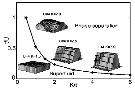
Figure 19: The phase diagram of soft-core bosons ($16\times 16$ Lattice). The phase is superfluid under the curve, while the system forms a cluster in the upper part. The curve is approximately hyperbolic.

Our phase diagram Fig. 19 is for half-filling, but the main feature, a tendency to phase separation, is the same at other densities. As an extreme example, simulations done for a commensurate filling of one particle per site show that, like the superfluid phase, the Mott phase also collapses when the ring exchange processes are too strong, and is replaced by clustering (Fig. 20).

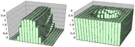
Figure 20: Density profiles for the soft-core case with $U=4$ and $K=8$ for commensurate fillings, $\rho=1$ (left) and $\rho=2$ (right).

Results: Soft-core case, $V\neq 0$

In the preceding two sections we have seen that a Bose-liquid does not occur in either the hard- or soft-core Bose Hubbard models when ring exchange is included, in contrast to recent suggestions.Paramekanti02 It is natural to consider whether longer range repulsion might prevent the system from collapsing. As a first step, we now include a repulsion between first nearest neighbors. Fig. 21 shows the structure factor $S(\pi,\pi)$ and $\Omega$ for $U=5t$ and different values of $V$, as a function of $K$ at half-filling. Three different behaviors of the density correlations are observable: a CDW (density order at momentum $(\pi,\pi)$) when $K$ is weak (well known in the model without ring exchange processes),Niyaz93 at intermediate $K$ a uniform phase where the density structure factor is small at all wavelengths, and a regime of phase separation ($\Omega$ large) when $K$ is big. As expected, $V$ does suppress the tendency for clustering. $K$ must be made larger for phase separation to occur when $V$ is increased. The phases of Fig. 21 are also directly visible in real space snapshots of the densities in the course of the simulations (Fig. 22).

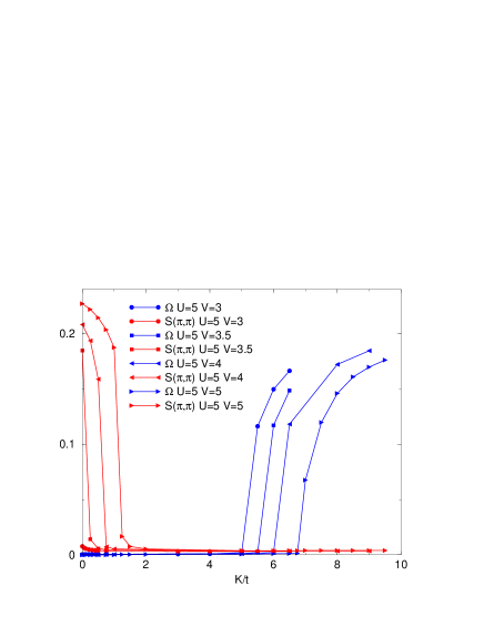
Figure 21: The CDW structure factor $S(\pi,\pi)$ and $\Omega$ for $U=5t$ and different values of the potential $V$ between first nearest neighbors, at half filling ($16\times 16$ Lattice). $V$ is seen to compete with phase separation, pushing the onset of the rise in $\Omega$ out to larger and larger $K$.

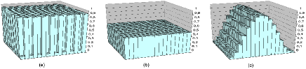
Figure 22: Density profiles at half filling for $U=5t$, $V=5t$, and different values of $K$: (a) $K=t$, CDW phase; (b) $K=5t$, uniform density; and (c) $K=7t$, phase separation.

Despite the absence of density order, the uniform phase (Fig. 22b) is not a Bose liquid. Fig. 23 shows that the superfluid density is zero only for the CDW phase. As soon as the staggered density order is destroyed with increasing $K$, the superfluid density becomes nonzero. $\rho_{s}$ climbs rapidly and is roughly constant through the region where both $S(\pi,\pi)$ and $\Omega$ are small. It remains non-zero in the cluster phase, though it does drop by a factor of two when clumping begins. There is no Bose liquid phase in the model. (Of course, if the density is sufficiently small, then an island phase in which the boson cloud does not span the system will have vanishing $\rho_{s}$. This situation also occurs for bosons in a confining potential, where the phase is nevertheless commonly referred to as being superfluid.

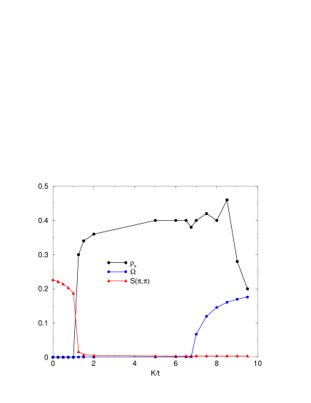
Figure 23: The superfluid density $\rho_{s}$, the structure factor $S(\pi,\pi)$, and $\Omega$ as functions of $K$ for $U=5t$ and $V=5t$ ($16\times 16$ Lattice). The superfluid density vanishes only when the system is in the CDW phase.

Conclusions

In this paper we have studied the effect of a ring exchange term in the hard- and soft-core Bose Hubbard model, also including a near-neighbor repulsion, using Quantum Monte Carlo simulations in the canonical ensemble. It had been suggested that this term might lead to a normal Bose liquid phase, that is, one which is compressible but non superfluid. For the Hard-core case, we reproduced results obtained by Melko et al. Melko04 in the grand canonical ensemble. However, working in the canonical ensemble enables us to capture and characterize a hitherto unsuspected cluster phase of the model. No Bose liquid phase was observed. Thus the speculation of Paramekanti et al Paramekanti02 , that the relaxation of the hard-core constraint might give rise to a Bose liquid does not appear to be borne out. The tendency to clustering can be understood by analyzing the effect of $K$ on a two boson system. We have shown numerically that $K$ acts much like an attractive potential, and that when it is sufficiently large, the two boson form a bound state. This attraction leads to clustering in systems with larger boson numbers.

We saw that, while a near neighbor repulsion competes with this clustering, it could not create a normal bose liquid. At weak $K$ it promotes an alternate charge density wave insulator. At strong $K$, while $V$ does help prevent clustering, $\rho_{s}$ remains nonzero. It might be interesting to study models with longer range interactions which will act together to prevent phase separation, but compete with each other by promoting phases at different ordering momenta. Such models might, finally, realize the Bose liquid phase.

To conclude, let us comment on the implications of our work for the phase diagram of the spin-1/2 quantum Heisenberg model with a ring exchange term. The kinetic energy term in the hard-core boson Hubbard model maps onto $J\sum(S_{{\bf i}}^{x}S_{{\bf j}}^{x}+S_{{\bf i}}^{y}S_{{\bf j}}^{y})$ with exchange constant $J=2t$. At the value $U=4t$ in our soft core model, double occupancy is already very rare at half-filling, and hence we are almost in the hard-core limit. The value of the ring exchange energy scale required to drive phase separation for this $U$ is $K\approx 2t$, or in other words, $K\approx J$. To reproduce the near-neighbor coupling of the $z$ components of spin in the Heisenberg model we must include a near-neighbor repulsion in the bose-Hubbard model, a term which clearly would suppress phase separation. Thus we expect ring exchange to have the potential to drive phase separation in the Heisenberg model only for $K$ considerably greater than $J$.

We acknowledge support from the National Science Foundation under awards NSF DMR 0312261 and NSF INT 0124863, and useful input from R. Stones.

References

- (1) D.J. Thouless, Proc. Phys.Soc. London 86, 893 (1965).
- (2) A. Paramekanti, L. Balents and M. P. A. Fisher, Phys. Rev. B66 054526 (2002).
- (3) S. Doniach and D. Das Brazilian Journal of Physics 33, 740 (2003).
- (4) R. Coldea, S.M. Hayden, G. Aeppli,T.G. Perring, C.D. Frost, T.E. Mason, S.W. Cheong, and Z. Fisk, Phys. Rev. Lett. 86, 5377 (2001).
- (5) A.A. Katanin and A.P. Kampf, Phys. Rev. B66, 100403(R) (2002).
- (6) E. Muller-Hartmann and A. Reischl, Eur. Phys. J. B28, 173 (2002).
- (7) R.G. Melko, A.W. Sandvik, and D.J. Scalapino, Phys. Rev. B69, 100408 (2004).
- (8) V. Rousseau, G. G. Batrouni, and R.T. Scalettar, Phys. Rev. Lett. 93, 110404 (2004).
- (9) G. Roux, S.R. White, D. Poilblanc, S. Capponi, and A. Laeuchli, cond-mat/0504027.
- (10) Kwon Park and Subir Sachdev, Phys. Rev. B 65, 220405(R) (2002).
-
(11)
A. Sandvik,
http://meetings.aps.org/Meeting/MAR05/Event/21550. - (12) H.P. Buchler, M. Hermele, S.D. Huber, M.P.A. Fisher, and P. Zoller, cond-mat/0503254.
- (13) M.P.A. Fisher, P.B. Weichman, G. Grinstein, and D.S. Fisher, Phys. Rev. B40, 546 (1989).
- (14) G.G. Batrouni, R.T. Scalettar, and G.T. Zimanyi, Phys. Rev. Lett. 65, 1765 (1990).
- (15) T.D. Kuhner, S.R. White, and H. Monien, Phys. Rev. B61, 12474 (2000).
- (16) J. K. Freericks and H. Monien Phys. Rev. B53, 2691 (1996).
- (17) W. Krauth and N. Trivedi, Europhys. Lett. 14, 627 (1991).
- (18) A. van Otterlo and K.-H. Wagenblast, Phys. Rev. Lett. 72, 3598 (1994).
- (19) For studies of a closely related current model, see A. Kuklov, N. Prokof’ev, and B. Svistunov Phys. Rev. Lett. 93, 230402 (2004), and references cited therein.
- (20) P. Niyaz, R.T. Scalettar, C.Y. Fong, and G.G. Batrouni, Phys. Rev. B44, 7143 (1991); P. Niyaz, R.T. Scalettar, C.Y. Fong, and G.G. Batrouni, Phys. Rev. B50, 362 (1994).
- (21) K.S. Liu and M.E. Fisher, J. Low Temp. Phys. 10, 655 (1973); H. Matsuda and T. Tsuneto, Suppl. Prog. Theor. Phys. 46, 411 (1970); G. Chester, Phys. Rev. A2, 256 (1970); E. Roddick and D.H. Stroud, Phys. Rev. B48, 16600 (1993); and A.V. Otterlo and K. Wagenblast, Phys. Rev. Lett. 72, 3598 (1994).
- (22) G.G. Batrouni, R.T. Scalettar, G.T. Zimanyi, and A.P. Kampf, Phys. Rev. Lett. 74 2527 (1995); G.G. Batrouni and R.T. Scalettar, Phys. Rev. Lett. 84, 1599 (2000);
- (23) E. Loh et al. Phys. Rev. B31 4712 (1985).
- (24) See for example, reference Batrouni90 where only two site decouplings were used.
- (25) A. W. Sandvik and J. Kurkijarvi, Phys. Rev. B43 5950 (1991).
- (26) R.M. Fye, Phys. Rev. B33, 6271 (1986).
- (27) R.M. Fye and R.T. Scalettar Phys. Rev. B36, 3833 (1987).
- (28) If one were interested in cases where the density were larger, and the on-site were small, this might no longer be a good approximation.
- (29) E.L. Pollock and D.M. Ceperley, Phys. Rev. B, 36, 8343 (1987).