A new hybrid LDA and Generalized Tight-Binding method for the electronic structure calculations of strongly correlated electron systems

Abstract

A novel hybrid scheme is proposed. The ab initio LDA calculation is used to construct the Wannier functions and obtain single electron and Coulomb parameters of the multiband Hubbard-type model. In strong correlation regime the electronic structure within multiband Hubbard model is calculated by the Generalized Tight-Binding (GTB) method, that combines the exact diagonalization of the model Hamiltonian for a small cluster (unit cell) with perturbation treatment of the intercluster hopping and interactions. For undoped La₂CuO₄ and Nd₂CuO₄ this scheme results in charge transfer insulators with correct values of gaps and dispersions of bands in agreement to the ARPES data.

I Introduction

A conventional band theory is based on the density functional theory (DFT) hohenberg1 and on the Local Density Approximation (LDA) kohn1 within DFT. In spite of great success of the LDA for conventional metallic systems it appears to be inadequate for strongly correlated electron systems (SCES). For instance, LDA predicts La₂CuO₄ to be a metal whereas, in reality, it is an insulator. Several approaches to include strong correlations in the LDA method are known, for example LDA+U anisimov1 and LDA-SIC svane1 . Both methods result in the correct antiferromagnetic insulator ground state for La₂CuO₄ contrary to LDA, but the origin of the insulating gap is not correct. It is formed by the local single-electron states splitted by spin or orbital polarization. In these approaches the paramagnetic phase of the undoped La₂CuO₄ (above the Neel temperature $T_{N}$ ) will be metallic in spite of strong correlation regime $U\gg W$, where $U$ is the Hubbard Coulomb parameterhubbard1 and $W$ is a free electron bandwidth. The spectral weight redistribution between Hubbard subbands is very important effect in SCES that is related to the formation of the Mott-Hubbard gap in the paramagnetic phase. This effect is incorporated in the hybrid LDA+dynamical mean field theory (DMFT) (for review see Ref.anisimov2 ; Held ; psik ) and LDA++ approaches. lichtenstein1 The electron self-energy in LDA+DMFT approach is calculated by the DMFT theory in the limit of infinite dimension voll93 ; phystoday and is k-independent, $\Sigma_{\bf k}\left(E\right)\to\Sigma\left(E\right)$. metzner1 ; georges1 That is why the correct band dispersion and the ARPES data for High-$T_{c}$ compounds cannot be obtained within LDA+DMFT theory. Recent development of the LDA+cluster DMFT method hettler1 ; TMrmp and spectral density functional theory savrasov1 gives some hopes that non-local corrections may be included in this scheme.

A generalized tight-binding (GTB) ovchinnikov1 method has been proposed to study the electronic structure of SCES as a generalization of Hubbard ideas for the realistic multiband Hubbard-like models. The GTB method combines the exact diagonalization of the intracell part of the Hamiltonian, construction of the Hubbard operators on the basis of the exact intracell multielectron eigenstates, and the perturbation treatment of the intercell hoppings and interactions. A similar approach to the 3-band $p-d$ model of cuprates emery1 ; varma1 is known as the cell perturbation method. lovtsov1 ; jefferson1 ; schutler1 The practical realization of the GTB method for cuprates required an explicit construction of the Wannier functions to overcome the nonorthogonality of the oxygen molecular orbitals at the neighboring $CuO_{6}$ cells. gavrichkov1 The GTB calculations for undoped and underdoped cuprates are in good agreement with ARPES data both in the dispersion of the valence band and in the spectral intensity. gavrichkov1 ; gavrichkov2 A strong redistribution of spectral weight with hole doping and the formation of the in-gap states have been obtained in these calculations. Similar GTB calculations for the manganites has been done recently. gavrichkov3

As any model Hamiltonian approach the GTB method is not ab initio, there are many Hamiltonian parameters like intraatomic energy levels of $p$ and $d$ electrons, various $p-d$ and $p-p$ hopping parameters, Coulomb and exchange interaction parameters. These parameters have been obtained by fitting the set of optical, magnetic ovchinnikov2 and ARPES gavrichkov1 data. Generally the question arises how unique the set of parameters is. To overcome this restriction we have proposed in this paper a novel LDA+GTB scheme that allows to calculate the GTB parameters by the ab initio LDA approach.

The paper is organized as follows: In Section II the construction of Wannier functions from self-consistent LDA eigenfunctions as well as ab initio parameters of the multiband $p-d$ model for La₂CuO₄ and Nd₂CuO₄ are given. A brief description of the GTB method is done in Section III. Section IV contains the LDA+GTB band structure calculations for La₂CuO₄ and Nd₂CuO₄. The effective low-energy $t-J$* model with ab initio parameters is presented in Section V. Section VI is the conclusion.

II Calculation of ab initio parameters from LDA

To obtain hopping integrals for different sets of bands included in consideration we apply projection procedure using Wannier functions (WFs) formalism. wf_anisimov WFs were first introduced in 1937 by Wannier wannier as Fourier transformation of Bloch states $|\psi_{i\bf k}\rangle$

$$|W_{i}^{\bf T}\rangle = \frac{1}{\sqrt{N}}\sum_{\bf k}e^{-i{\bf kT}}|\psi_{i{\bf k}}\rangle,$$ (1)

where T is lattice translation vector, $N$ is the number of discrete ${\bf k}$ points in the first Brillouin zone and $i$ is band index. One major reason why the WFs have seen little practical use in solid-state applications is their nonuniqueness since for a certain set of bands any orthogonal linear combination of Bloch functions $|\psi_{i\bf k}\rangle$ can be used in (1). Therefore to define them one needs an additional constraint. Among others Marzari and Vanderbilt vanderbildt proposed the condition of maximum localization for WFs, resulting in a variational procedure. To get a good initial guess authors of Ref.vanderbildt, proposed to choose a set of localized trial functions $|\phi_{n}\rangle$ and project them onto the Bloch states $|\psi_{i\bf k}\rangle$. It was found that this starting guess is usually quite good. This fact later led to the simplified calculating scheme pickett where the variational procedure was abandoned as in present work and the result of the aforementioned projection was considered as the final step.

II.1 Wannier function formalism

To construct the WFs one should to define a set of trial orbitals $|\phi_{n}\rangle$ and choose the Bloch functions of interest by band indexes (N₁, …, N₂) or by energy interval ($E_{1},E_{2}$). Non-orthogonalized WFs in reciprocal $|\widetilde{W}_{n\bf k}\rangle$ space are then the projection of the set of site-centered atomic-like trial orbitals $|\phi_{n}\rangle$ on the Bloch functions $|\psi_{i\bf k}\rangle$ of the chosen bands:

$$|\widetilde{W}_{n\bf k}\rangle \equiv \sum_{i(E_{1}\leq\epsilon_{i}({\bf k})\leq E_{2})}|\psi_{i\bf k}\rangle\langle\psi_{i\bf k}|\phi_{n}\rangle,$$ (2)

where $\epsilon_{i}({\bf k})$ is the band dispersion of $i$-th band obtained from self-consistent ab initio LDA calculation. In present work we use LMT-orbitals lmto as trial functions. The Bloch functions in LMTO basis are defined as

$$|\psi_{i\bf k}\rangle = \sum_{\mu}c^{\bf k}_{\mu i}|\phi_{\mu}^{\bf k}\rangle,$$ (3)

where $\mu$ is the combined index representing $qlm$ ($q$ is the atomic number in the unit cell, $l$ and $m$ are orbital and magnetic quantum numbers), $\phi_{\mu}^{\bf k}({\bf r})$ are the Bloch sums of the basis orbitals $\phi_{\mu}({\bf r-T})$

$$\phi_{\mu}^{\bf k}({\bf r}) = \frac{1}{\sqrt{N}}\sum_{\bf T}e^{i\bf kT}\phi_{\mu}({\bf r}-{\bf T}),$$ (4)

and the coefficients are

$$c^{\bf k}_{\mu i}=\langle\phi_{\mu}|\psi_{i\bf k}\rangle.$$ (5)

Since in present work $|\phi_{n}\rangle$ is an orthogonal LMTO basis set orbital (in other words $n$ in $|\phi_{n}\rangle$ corresponds to the particular $qlm$ combination), then $\langle\psi_{i\bf k}|\phi_{n}\rangle=c_{ni}^{{\bf k}*}$. Hence

$$|\widetilde{W}_{n\bf k}\rangle = \sum_{i=N_{1}}^{N_{2}}|\psi_{i\bf k}\rangle c_{ni}^{{\bf k}*}=\sum_{i=N_{1}}^{N_{2}}\sum_{\mu}c^{\bf k}_{\mu i}c_{ni}^{{\bf k}*}|\phi_{\mu}^{\bf k}\rangle.$$ (6)

In order to orthonormalize the WFs (6) one needs to calculate the overlap matrix $O_{nn^{\prime}}({\bf k})$

$$O_{nn^{\prime}}({\bf k}) \equiv \langle\widetilde{W}_{n\bf k}|\widetilde{W}_{n^{\prime}\bf k}\rangle=\sum_{i=N_{1}}^{N_{2}}c^{\bf k}_{ni}c_{n^{\prime}i}^{{\bf k}*},$$ (7)

then its inverse square root $S_{nn^{\prime}}({\bf k})$ is defined as

$$S_{nn^{\prime}}({\bf k}) \equiv O^{-1/2}_{nn^{\prime}}({\bf k}).$$ (8)

In the derivation of (7) the orthogonality of Bloch states $\langle\psi_{n\bf k}|\psi_{n^{\prime}\bf k}\rangle=\delta_{nn^{\prime}}$ was used.

From (6) and (8), the orthonormalized WFs in ${\bf k}$-space $|W_{n\bf k}\rangle$ can be obtained as

$$|W_{n\bf k}\rangle=\sum_{n^{\prime}}S_{nn^{\prime}}({\bf k})|\widetilde{W}_{n^{\prime}\bf k}\rangle=\sum_{i=N_{1}}^{N_{2}}|\psi_{i\bf k}\rangle\bar{c}_{ni}^{{\bf k}*}$$ ,

$$\bar{c}_{ni}^{{\bf k}*}\equiv\langle\psi_{i\bf k}|W_{n\bf k}\rangle=\sum_{n^{\prime}}S_{nn^{\prime}}({\bf k})c_{n^{\prime}i}^{{\bf k}*}.$$

Then the matrix element of the Hamiltonian $\widehat{H}^{WF}$ in reciprocal space is

$$H^{WF}_{nn^{\prime}}({\bf k}) = \langle W_{n\bf k}|\biggl{(}\frac{1}{N}\sum_{\bf k^{\prime}}\sum_{i=N_{1}}^{N_{2}}|\psi_{i\bf k^{\prime}}\rangle\epsilon_{i}({\bf k^{\prime}})\langle\psi_{i\bf k^{\prime}}|\biggr{)}|W_{n^{\prime}\bf k}\rangle$$ (9)

$$= \sum_{i=N_{1}}^{N_{2}}\bar{c}^{\bf k}_{ni}\bar{c}_{n^{\prime}i}^{{\bf k}*}\epsilon_{i}({\bf k}).$$

Hamiltonian matrix element in real space is

$$H^{WF}_{nn^{\prime}}(\bf T) = \langle W_{n}^{\bf 0}|\hat{H}|W_{n^{\prime}}^{\bf T}\rangle=\frac{1}{N}\sum_{\bf k}\sum_{i=N_{1}}^{N_{2}}\bar{c}^{\bf k}_{ni}\bar{c}_{n^{\prime}i}^{{\bf k}*}\epsilon_{i}({\bf k})e^{-i\bf kT},$$

here atom $n^{\prime}$ is shifted from its position in the primary unit cell by a translation vector ${\bf T}$. For more detailed description of this procedure see. wf_anisimov

II.2 LDA band structure, hopping and Coulomb parameters for p- and n-type cuprates

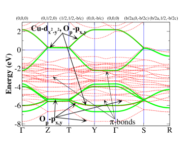
Figure 1: (Color online) Comparison of the band structure of La₂CuO₄ from LDA calculation (dotted lines) and from projection on the Cu-$d_{x^{2}-y^{2}}$ and O_p-$p_{x}$, O_p-$p_{y}$ set of orbitals (bold solid lines). Fermi level coresponds to zero energy.

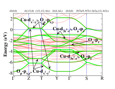
Figure 2: (Color online) The same as in Fig. 1 but projection is done on the Cu-$d_{x^{2}-y^{2}}$, Cu-$d_{3z^{2}-r^{2}}$ and O_p-$p_{x}$, O_p-$p_{y}$, O_a-$p_{z}$ set of orbitals.

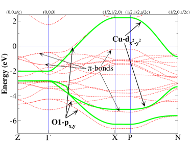
Figure 3: (Color online) Comparison of the band structure of Nd₂CuO₄ from LDA calculation (dotted lines) and from projection on the Cu-$d_{x^{2}-y^{2}}$, O1-$p_{x}$ and O1-$p_{y}$ set of orbitals (bold solid lines). Fermi level corresponds to zero energy.

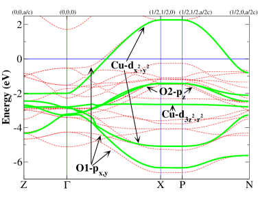
Figure 4: (Color online) The same as in Fig. 3 but projection is done on the Cu-$d_{x^{2}-y^{2}}$, Cu-$d_{3z^{2}-r^{2}}$ and O1-$p_{x}$, O1-$p_{y}$, O2-$p_{z}$ set of orbitals.

Basically all cuprates have one or more CuO₂ planes in their structure, which are separated by layers of other elements (Ba, Nd, La, …). They provide the carriers in CuO₂ plane and according to the type of carriers all cuprates can be divided into two classes: p-type and n-type. In present paper we deal with the simplest representatives of this two classes: La_2-xSr_xCuO₄ (LSCO) and Nd_2-xCe_xCuO₄ (NCCO) correspondingly.

LDA band calculation for La₂CuO₄ and Nd₂CuO₄ was done within LMTO method lmto using atomic sphere approximation in tight-binding approach tblmto (TB-LMTO-ASA). In the case of Nd₂CuO₄ Nd-4$f$ states were treated as pseudocore states.

La₂CuO₄ at the low temperature and zero doping has the orthorhombic structure (LTO) with the space group $Bmab$. strucLa The lattice parameters and atomic cordinates at 10 K were taken from Ref.strucLa, to be a=5.3346, b=5.4148 and c=13.1172 Å, La (0, -0.0083, 0.3616), Cu (0, 0, 0), O_p (0.25, 0.25, -0.0084), O_a (0, 0.0404, 0.1837). Here and below O_p denotes in-plane oxygen ions and O_a - apical oxygen ions. In comparison with high temerature teragonal structure (HTT) orthorhombic La₂CuO₄ have two formula units per unit cell and the CuO₆ octahedra are rotated cooperatively about the [110] axis. As a result O_p ions are slightly moved off the Cu plane and four in–plane La-O_a bond lengths are unequal.

Nd₂CuO₄ at the room temperature and zero doping has the tetragonal structure with the space group $I4/mmm$ strucNd also called T’-structure. The lattice parameters are a=b=3.94362, c=12.1584 Å. strucNd Cu ions at the 2a site (0, 0, 0) are surrounded by four oxygen ions O1 which occupy 4c position (0, 1/2, 0). The Nd at the 4e site (0, 0, 0.35112) have eight nearest oxygen ions neighbors O2 at 4d position (0, 1/2, 1/4). strucNd One can imagine body-centered T’-structure as the HTT structure of La₂CuO₄ but with two oxygen atoms moved from apices of each octahedron to the face of the cell at the midpoints between two oxygen atoms on the neighbouring CuO₂ planes. In other words Nd₂CuO₄ in T’-structure has no apical oxygens around Cu ion.

The LDA band structure of both compounds along the high-symmetry lines in the Brillouin zone is shown in Figs. 1-4 by dotted lines. The coordinates of high-symmetry points in BZ are given on top of each picture. The complex of bands in the energy range (-8, 2.5) eV consists primarily of Cu-$3d$ and O-$2p$ states. The total bandwidths amount 10 eV for La-cuprate and 7 eV for Nd-cuprate. Contribution of Cu-$3d$ and O-$2p$ orbitals to the different bands is displayed by arrows.

One can see that the band crossing E_F have character of Cu-$d_{x^{2}-y^{2}}$ and O_p-$p_{x,y}$ for La₂CuO₄ and Cu-$d_{x^{2}-y^{2}}$, O1-$p_{x,y}$ in the case of Nd₂CuO₄. It corresponds to antibonding $pd\sigma$ orbital. So for hoppings calculation the projection on Cu-$d_{x^{2}-y^{2}}$, O_p-$p_{x}$, O_p-$p_{y}$ orbitals for La-cuprate and Cu-$d_{x^{2}-y^{2}}$, O1-$p_{x}$, O1-$p_{y}$ orbitals for Nd-cuprate was done. Such set of orbitals corresponds to the 3-band $p-d$ model. The bands obtained by the described in Sec. II.1 projection procedure are shown by solid lines in Figs. 1 and 3. It is clearly seen that in case of La₂CuO₄ 3-band model did not reproduce the band crossing E_F properly (Fig. 1, SR direction).

Since 3-band $p-d$ model didn’t provide proper description of the LDA bands around Fermi level the projection on more complex set of trail orbitals for both compounds was done. The resulting bands are plotted by solid lines in Figs. 2 and 4. Corresponding multiband $p-d$ model contains Cu-$d_{x^{2}-y^{2}}$, Cu-$d_{3z^{2}-r^{2}}$, O_p-$p_{x}$, O_p-$p_{y}$, O_a-$p_{z}$ states for La₂CuO₄ and Cu-$d_{x^{2}-y^{2}}$, Cu-$d_{3z^{2}-r^{2}}$, O1-$p_{x}$, O1-$p_{y}$, O2-$p_{z}$ states for Nd₂CuO₄. The energy range for projection was (-8.4, 2.5) eV and (-8, 2) eV for the case of La-cuprate and Nd-cuprate correspondingly. The main effect of taking into account Cu-$d_{3z^{2}-r^{2}}$ and O_a-$p_{z}$ states for La₂CuO₄ is the proper description of the band structure (in comparison with LDA calculation) at the energies up to 2 eV below Fermi level. From Fig. 3 and 4 one can see that in case of Nd₂CuO₄ both sets of trial orbitals properly describe the LDA band crossing the Fermi level which has Cu-$d_{x^{2}-y^{2}}$ symmetry. At the same time its bonding part does not agree well with the LDA bands since projection did not include all Cu-$d$ and O-$p$ orbitals.

Table 1: Hopping parameters and single electron energies for orthorhombic La₂CuO₄ obtained in WF projection procedure for different sets of trial orbitals (all values in eV). Here $x^{2}$, $z^{2}$, $p_{x}$, $p_{y}$, $p_{z}$ denote Cu-$d_{x^{2}-y^{2}}$, Cu-$d_{3z^{2}-r^{2}}$, O_p-$p_{x}$, O_p-$p_{y}$, O_a-$p_{z}$ orbitals correspondingly. The 3-d and 4-th columns correspond to bases of the 3-band and the multiband $p-d$ models respectively.

Hopping	Connecting	Cu-$x^{2}$	Cu-$x^{2}$, $z^{2}$
	vector	O $p_{x}$, $p_{y}$	O-$p_{x}$, $p_{y}$, $p_{z}$
		E${}_{x^{2}}$=-1.849	E${}_{x^{2}}$=-1.849
		E${}_{p_{x}}$=-2.767	E${}_{z^{2}}$=-2.074
		E${}_{p_{y}}$=-2.767	E${}_{p_{x}}$=-2.806
			E${}_{p_{y}}$=-2.806
			E${}_{p_{z}}$=-1.676
t($x^{2}$,$x^{2}$)	(-0.493,-0.5)	-0.188	-0.188
t′($x^{2}$,$x^{2}$)	(-0.985, 0.0)	0.001	0.002
t($z^{2}$,$z^{2}$)	(-0.493,-0.5)		0.054
t′($z^{2}$,$z^{2}$)	(-0.985, 0.0)		-0.001
t($x^{2}$,$p_{x}$)	(0.246,0.25,-0.02)	1.357	1.355
t′($x^{2}$,$p_{x}$)	(-0.739,0.25,-0.02)	-0.022	-0.020
t($z^{2}$,$p_{x}$)	(0.246,0.25,-0.02)		-0.556
t′($z^{2}$,$p_{x}$)	(-0.739,0.25,-0.02)		-0.028
t($z^{2}$,$p_{z}$)	(0,0.04,0.445)		0.773
t′($z^{2}$,$p_{z}$)	(-0.493,-0.46,-0.445)		-0.011
t($p_{x}$,$p_{y}$)	(0.493, 0.0)	-0.841	-0.858
t′($p_{x}$,$p_{y}$)	(0,0.5,0.041)	0.775	0.793
t′′($p_{x}$,$p_{y}$)	(0.985,0.5,0.041)	-0.001	-0.001
t($p_{x}$,$p_{z}$)	(-0.246,-0.21,0.465)		-0.391
t′($p_{x}$,$p_{z}$)	(0.246,0.29,-0.425)		-0.377
t′′($p_{x}$,$p_{z}$)	(0.246,-0.21,-0.746)		0.018

Table 2: Hopping parameters and single electron energies for Nd₂CuO₄ obtained in WF projection procedure for different sets of trial orbitals (all values in eV). Here $x^{2}$, $z^{2}$, $p_{x}$, $p_{y}$, $p_{z}$ denote Cu-$d_{x^{2}-y^{2}}$, Cu-$d_{3z^{2}-r^{2}}$, O1-$p_{x}$, O1-$p_{y}$, O2-$p_{z}$ orbitals correspondingly. The 3-d and 4-th columns correspond to bases of the 3-band and the multiband $p-d$ models respectively.

Hopping	Connecting	Cu-$x^{2}$,	Cu-$x^{2}$, $z^{2}$,
	vector	O $p_{x}$, $p_{y}$	O-$p_{x}$, $p_{y}$, $p_{z}$
		E${}_{x^{2}}$=-1.989	E${}_{x^{2}}$=-1.991
		E${}_{p_{x}}$=-3.409	E${}_{z^{2}}$=-2.778
		E${}_{p_{y}}$=-3.409	E${}_{p_{x}}$=-3.368
			E${}_{p_{z}}$=-2.30
t($x^{2}$,$x^{2}$)	(1, 0)	0.01	0.01
t′($x^{2}$,$x^{2}$)	(1, 1)	-0.00	-0.00
t($z^{2}$,$z^{2}$)	(1, 0)		0.01
t′($z^{2}$,$z^{2}$)	(1, 1)		0.00
t($x^{2}$,$p_{x}$)	(0.5,0)	1.18	1.18
t′($x^{2}$,$p_{x}$)	(0.5,1)	-0.06	-0.06
t′($x^{2}$,$p_{x}$)	(1.5,0)	0.04	0.04
t′′′($x^{2}$,$p_{x}$)	(1.5,1)	0.00	0.00
t($z^{2}$,$p_{x}$)	(0.5,0)		-0.29
t′($z^{2}$,$p_{x}$)	(0.5, 1)		0.01
t($z^{2}$,$p_{z}$)	(0, 0.5, 0.771)		0.10
t′($z^{2}$,$p_{z}$)	(1, 0.5, 0.771)		0.02
t($p_{x}$,$p_{y}$)	(0.5,0.5)	0.69	0.67
t′($p_{x}$,$p_{y}$)	(1.5,0.5)	0.00	0.00
t($p_{x}$,$p_{z}$)	(0.5, 0.5, 0.771)		0.02
t′($p_{x}$,$p_{z}$)	(0.5,-0.5, 0.771)		0.02

The resulting hopping parameters and energy of particular orbitals for two sets of trial orbitals are presented in Tables  1 and 2. The second column contains the connecting vector T between two sites. It is clearly seen that hoppings decay quite rapidly with distance between ions.

For the multiband $p-d$ model the values of Coulomb parameters are also required. For Cu in La₂CuO₄ they were obtained in constrained LDA supercell calculations constrain to be $U=10$ eV and $J=1$ eV. sorella For the Nd₂CuO₄ we will use the same values of these parameters.

III GTB method overview

As the starting model that reflects chemical structure of the cuprates it is convenient to use the 3-band $p-d$ model emery1 ; varma1 or the multiband $p-d$ model. gaididei1 While the first one is simplier it lacks for some significant features, namely importance of $d_{z^{2}}$ orbitals on copper and $p_{z}$ orbitals on apical oxygen. Non-zero occupancy of $d_{z^{2}}$ orbitals pointed out in XAS and EELS experiments which shows 2-10% occupancy of $d_{z^{2}}$ orbitals bianconi1 ; romberg1 and 15% doping dependent occupancy of $p_{z}$ orbitals chen1 in all hole doped High-$T_{c}$ compounds). Henceforth the multiband $p-d$ model will be used.

Let us consider the Hamiltonian with the following general structure:

$$H = \sum\limits_{f,\lambda,\sigma}(\epsilon_{\lambda}-\mu)n_{f\lambda\sigma}+\sum\limits_{f\neq g}\sum\limits_{\lambda,\lambda^{\prime},\sigma}T_{fg}^{\lambda\lambda^{\prime}}c_{f\lambda\sigma}^{\dagger}c_{g\lambda^{\prime}\sigma}$$ (10)

$$+ \frac{1}{2}\sum\limits_{f,g,\lambda,\lambda^{\prime}}\sum\limits_{\sigma_{1,2,3,4}}V_{fg}^{\lambda\lambda^{\prime}}c_{f\lambda\sigma_{1}}^{\dagger}c_{f\lambda\sigma_{3}}c_{g\lambda^{\prime}\sigma_{2}}^{\dagger}c_{g\lambda^{\prime}\sigma_{4}},$$

where $c_{f\lambda\sigma}$ is the annihilation operator in Wannier representation of the hole at site $f$ at orbital $\lambda$ with spin $\sigma$, $n_{f\lambda\sigma}=c_{f\lambda\sigma}^{\dagger}c_{f\lambda\sigma}$.

In particular case of cuprates and corresponding multiband $p-d$ model, $f$ runs through copper and oxygen sites, index $\lambda$ run through $d_{x^{2}-y^{2}}\equiv d_{x^{2}}$ and $d_{3z^{2}-r^{2}}\equiv d_{z^{2}}$ orbitals on copper, $p_{x}$ and $p_{y}$ atomic orbitals on the O_p-oxygen sites and $p_{z}$ orbital on the apical O_a-oxygen; $\epsilon_{\lambda}$ - single-electron energy of the atomic orbital $\lambda$. $T_{fg}^{\lambda\lambda^{\prime}}$ includes matrix elements of hoppings between copper and oxygen ($t_{pd}$ for hopping $d_{x^{2}}\leftrightarrow p_{x},p_{y}$; $t_{pd}/\sqrt{3}$ for $d_{z^{2}}\leftrightarrow p_{x},p_{y}$; $t^{\prime}_{pd}$ for $d_{z^{2}}\leftrightarrow p_{z}$) and between oxygen and oxygen ($t_{pp}$ for hopping $p_{x}\leftrightarrow p_{y}$; $t^{\prime}_{pp}$ for hopping $p_{x},p_{y}\leftrightarrow p_{z}$). The Coulomb matrix elements $V_{fg}^{\lambda\lambda^{\prime}}$ includes intraatomic Hubbard repulsions of two holes with opposite spins on one copper and oxygen orbital ($U_{d}$, $U_{p}$), between different orbitals of copper and oxygen ($V_{d}$, $V_{p}$), Hund exchange on copper and oxygen ($J_{d}$, $J_{p}$) and the nearest-neighbor copper-oxygen Coulomb repulsion $V_{pd}$.

GTB method ovchinnikov1 ; gavrichkov1 ; gavrichkov2 consist of exact diagonalization of intracell part of the multiband Hamiltonian (10) and perturbative account of the intercell part. For La_2-xSr_xCuO₄ and Nd_2-xCe_xCuO₄ the unit cells are CuO₆ and CuO₄ clusters, respectively, and a problem of nonorthogonality of the molecular orbitals of adjacent cells is solved by an explicit fashion using the diagonalization in k-space raimondi1 . In a new symmetric basis the intracell part of the total Hamiltonian is diagonalized, allowing to classify all possible effective quasiparticle excitations in CuO₂-plane according to a symmetry. To describe this process the Hubbard X-operators hubbard2 $X_{f}^{m}\leftrightarrow X_{f}^{p,q}\equiv\left|p\right\rangle\left\langle q\right|$ are introduced. Index $m\leftrightarrow\left({p,q}\right)$ enumerates quasiparticle with energy $\omega_{m}=\varepsilon_{p}\left({N+1}\right)-\varepsilon_{q}\left(N\right)$, where $\varepsilon_{p}$ is the $p$-th energy level of the $N$-electron system. There is a correspondence between Hubbard operators and single-electron creation and annihilation operators:

$$c_{f\lambda\sigma}=\sum\limits_{m}\gamma_{\lambda\sigma}\left(m\right)X_{f}^{m},$$ (11)

where $\gamma_{\lambda\sigma}\left(m\right)$ determines the partial weight of a quasiparticle $m$ with spin $\sigma$ and orbital index $\lambda$. Using this correspondence we rewrite the Hamiltonian (10)

$$H=\sum\limits_{f,p}\left(\varepsilon_{p}-N\mu\right)X^{p,p}_{f}+\sum\limits_{f\neq g}\sum\limits_{m,m^{\prime}}t_{fg}^{mm^{\prime}}{X_{f}^{m}}^{\dagger}X_{g}^{m^{\prime}}.$$ (12)

This Hamiltonian, actually, have the form of the multiband Hubbard model.

Diagonalization of the Hamiltonian (10) mentioned above gives energies $\varepsilon_{p}$ and the basis of Hubbard operators $X_{f}^{m}$. Values of the hoppings,

$$t_{fg}^{mm^{\prime}}=\sum\limits_{\sigma,\lambda,\lambda^{\prime}}T_{fg}^{\lambda\lambda^{\prime}}\gamma^{\ast}_{\lambda\sigma}\left(m\right)\gamma_{\lambda^{\prime}\sigma}\left(m^{\prime}\right),$$ (13)

are calculated straightforwardly using the exact diagonalization of the intracell part of the Hamiltonian (10).

Again, in particular case of multiband $p-d$ model, the essential for cuprates multielectron configurations are $d^{10}p^{6}$ (vacuum state $\left|0\right\rangle$ in a hole representation), single-hole configurations $d^{9}p^{6}$, $d^{10}p^{5}$, and two-hole configurations $d^{8}p^{6}$, $d^{9}p^{5}$, $d^{10}p^{4}$, $d^{10}p^{5}p^{5}$. In the single-hole sector of the Hilbert space the $b_{1g}$ molecular orbital, that we will denote later as $\left|\sigma\right>=\left\{\left|\uparrow\right>,\left|\downarrow\right>\right\}$, has the minimal energy. In the two-hole sector the lowest energy states are singlet state $\left|S\right>$ with ${}^{1}A_{1g}$ symmetry, that includes Zhang-Rice singlet among other local singlets, and triplet states $\left|T\right>=\left|TM\right>$ ($M=+1,0,-1$) with ${}^{3}B_{1g}$ symmetry. gavrichkov1 ; gavrichkov2 ; raimondi1 All these states form the basis of the Hamiltonian (12), and they are shown together with quasiparticle excitations between them in the Fig. 5.

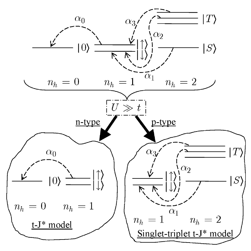
Figure 5: Schematic picture of states and quasiparticle excitations between them in Hubbard-type model (12). Here $n_{h}$ stands for number of holes, $\alpha_{i}$ numerates Fermi-type quasiparticles, states $\left|0\right>$, $\left|\sigma\right>$, $\left|S\right>$, $\left|T\right>$ represents basis of the Hamiltonian (12). Also, bases of effective models are shown.

In this basis relations (11) between annihilation-creation operators $c_{f\lambda\sigma}$ and Hubbard X-operators $X_{f}^{m}$ are

$$c_{fd_{x^{2}}\sigma}=uX_{f}^{0,\sigma}+2\sigma\gamma_{x}X_{f}^{\bar{\sigma},S},$$

$$c_{fp_{b}\sigma}=vX_{f}^{0,\sigma}+2\sigma\gamma_{b}X_{f}^{\bar{\sigma},S},$$

$$c_{fp_{a}\sigma}=\gamma_{a}(\sigma\sqrt{2}X_{f}^{\bar{\sigma},T0}-X_{f}^{\sigma,T2\sigma}),$$

$$c_{fd_{z^{2}}\sigma}=\gamma_{z}(\sigma\sqrt{2}X_{f}^{\bar{\sigma},T0}-X_{f}^{\sigma,T2\sigma}),$$

$$c_{fp_{z}\sigma}=\gamma_{p}(\sigma\sqrt{2}X_{f}^{\bar{\sigma},T0}-X_{f}^{\sigma,T2\sigma}),$$

and the explicit form of the Hamiltonian (12) is given by

$$H_{pd}=\sum_{f}\Bigl{[}\varepsilon_{1}\sum_{\sigma}X_{f}^{\sigma,\sigma}+\varepsilon_{2S}X_{f}^{S,S}+\varepsilon_{2T}\sum_{M}X_{f}^{TM,TM}\Bigl{]}$$

$$+\sum_{f\neq g,\sigma}\Bigl{[}t_{fg}^{00}X_{f}^{\sigma,0}X_{g}^{0,\sigma}+t_{fg}^{SS}X_{f}^{S,\bar{\sigma}}X_{g}^{\bar{\sigma},S}$$

$$+2\sigma t_{fg}^{0S}\left(X_{f}^{\sigma,0}X_{g}^{\bar{\sigma},S}+h.c.\right)$$

$$+t_{fg}^{ST}\left\{(\sigma\sqrt{2}X_{f}^{T0,\bar{\sigma}}-X_{f}^{T2\sigma,\sigma})(vX_{g}^{0,\sigma}+2\sigma\gamma_{b}X_{g}^{\bar{\sigma},S})+h.c.\right\}$$

$$+t_{fg}^{TT}(\sigma\sqrt{2}X_{f}^{T0,\bar{\sigma}}-X_{f}^{T2\sigma,\sigma})(\sigma\sqrt{2}X_{g}^{\bar{\sigma},T0}-X_{g}^{\sigma,T2\sigma})\Bigl{]}.$$ (14)

Here $\bar{\sigma}\equiv-\sigma$. The relation between effective hoppings (13) in this Hamiltonian and microscopic parameters of the multiband $p-d$ model is as follows korshunov2 ; korshunov3 :

$$t_{fg}^{00} = -2t_{pd}\mu_{fg}2uv-2t_{pp}\nu_{fg}v^{2},$$

$$t_{fg}^{SS} = -2t_{pd}\mu_{fg}2\gamma_{x}\gamma_{b}-2t_{pp}\nu_{fg}\gamma_{b}^{2},$$

$$t_{fg}^{0S} = -2t_{pd}\mu_{fg}(v\gamma_{x}+u\gamma_{b})-2t_{pp}\nu_{fg}v\gamma_{b},$$ (15)

$$t_{fg}^{TT} = \frac{2t_{pd}}{\sqrt{3}}\lambda_{fg}2\gamma_{a}\gamma_{z}+2t_{pp}\nu_{fg}\gamma_{a}^{2}-2t^{\prime}_{pp}\lambda_{fg}2\gamma_{p}\gamma_{a},$$

$$t_{fg}^{ST} = \frac{2t_{pd}}{\sqrt{3}}\xi_{fg}\gamma_{z}+2t_{pp}\chi_{fg}\gamma_{a}-2t^{\prime}_{pp}\xi_{fg}\gamma_{p}.$$

The factors $\mu$, $\nu$, $\lambda$, $\xi$, $\chi$ are the coefficients of Wannier transformation made in the GTB method and $u$, $v$, $\gamma_{x}$, $\gamma_{b}$, $\gamma_{a}$, $\gamma_{p}$, $\gamma_{z}$ are the matrix elements of annihilation-creation operators in the Hubbard X-operators representation gavrichkov1 .

Calculations gavrichkov1 ; gavrichkov2 of the quasiparticle dispersion and spectral intensities in the framework of the multiband $p-d$ model by the GTB method are in very good agreement to the ARPES data on insulating compound Sr₂CuO₂Cl₂. wells1 ; durr1 Other significant results of this method are borisov1 ; borisov2 :

i) pinning of Fermi level in LSCO at low concentrations was obtained in agreement with experiments. ino1 ; harima1 This pinning appears due to the in-gap state, spectral weight of this state is proportional to doping concentration $x$ and when Fermi level comes to this in-gap band then Fermi level “pins” there. The localized in-gap state exist in NCCO also for the same reason as in LSCO, but its energy is determined by the extremum of the band at $(\pi/2,\pi/2)$ point and it appears to be above the bottom of the conductivity band. Thus, the first doped electron goes into the band state at the $(\pi,0)$ and the chemical potential $\mu$ for the very small concentration merges into the band. At higher $x$ it meets the in-gap state with a pinning at $0.08<x<0.18$ and then $\mu$ again moves into the band. The dependence $\mu(x)$ for NCCO is quite asymmetrical to the LSCO and also agrees with experimental data; harima1

ii) experimentally observed ino2 evolution of Fermi surface with doping from hole-type (centered at $(\pi,\pi)$) in the underdoped region to electron-type (centered at $(0,0)$) in the overdoped region is qualitatively reproduced;

iii) pseudogap feature for LSCO is obtained as a lowering of density of states between the in-gap state and the states at the top of the valence band.

In all these calculations the set of the microscopic model parameters, obtained by fitting to experimental ARPES data, wells1 ; armitage1 was used. Hoppings and single-electron energies are listed in Table 3, values of Coulomb parameters are as follows:

$$\begin{array}[]{l}U_{d}=V_{d}=9,U_{p}=V_{p}=4,\\ J_{d}=1,J_{p}=0,V_{pd}=1.5.\end{array}$$ (18)

Table 3: Hopping parameters and single-electron energies of holes obtained by fitting GTB band structure to experimental data and in the ab initio calculations for p- and n-type cuprates (all values in eV).

	p-type		n-type
	fitted	ab initio	fitted	ab initio
$\varepsilon_{d_{x^{2}}}$	0	0	0	0
$\varepsilon_{p_{x}}$	1.5	0.91	1.4	1.38
$\varepsilon_{d_{z^{2}}}$	0.2	0.14	0.5	0.79
$\varepsilon_{p_{z}}$	0.45	-0.26	0.45	0.31
$t_{pd}$	1	1	1	1
$t_{pp}$	0.46	0.63	0.56	0.57
$t^{\prime}_{pd}$	0.58	0.57	0	0.08
$t^{\prime}_{pp}$	0.42	0.29	0.1	0.02

All results above were obtained treating the intercell hopping in the Hubbard-I approximation. hubbard1 But the GTB method is not restricted to such a crude approximation. The Fourier transform of the two-time retarded Green function in energy representation can be rewritten in terms of matrix Green function $D_{k\sigma}^{mn}\left(E\right)=\left<\left<X_{k\sigma}^{m}\left|{X_{k\sigma}^{n}}^{\dagger}\right.\right>\right>_{E}$:

$$\left<\left<c_{k\lambda\sigma}\left|c_{k\lambda\sigma}^{\dagger}\right.\right>\right>_{E}=\sum\limits_{m,m^{\prime}}\gamma_{\lambda\sigma}\left(m\right)\gamma_{\lambda\sigma}^{\ast}\left(m^{\prime}\right)D_{k\sigma}^{mm^{\prime}}\left(E\right).$$

The diagram technique for Hubbard X-operators is developed zaitsev1 ; izumov1 and the generalized Dyson equation ovchinnikov_book1 reads:

$$\hat{D}_{k\sigma}\left(E\right)=\left\{{\left[{\hat{G}_{k\sigma}^{(0)}\left(E\right)}\right]^{-1}+\hat{\Sigma}_{k\sigma}\left(E\right)}\right\}^{-1}\hat{P}_{k\sigma}\left(E\right).$$ (19)

Here, $\hat{\Sigma}_{k\sigma}\left(E\right)$ and $\hat{P}_{k\sigma}\left(E\right)$ are the self-energy and the strength operators, respectively. The presence of the strength operator is due to the redistribution of the spectral weight, that is an intrinsic feature of SCES. First time it was introduced in the spin diagram technique and called “a strength operator” baryakhtar_book1 because the value of $\hat{P}_{k\sigma}\left(E\right)$ determines an oscillator strength of excitations. It is also should be stressed, that $\hat{\Sigma}_{k\sigma}\left(E\right)$ in Eq. (19) is the self-energy in X-operators representation and therefore it is different from the self-energy entering Dyson equation for the Green function $\left<\left<c_{k\lambda\sigma}\left|c_{k\lambda\sigma}^{\dagger}\right.\right>\right>_{E}$. The Green function $\hat{G}_{k\sigma}^{(0)}\left(E\right)$ is defined by the formula

$$\left[{\hat{G}_{k\sigma}^{(0)}\left(E\right)}\right]^{-1}=\hat{G}_{0}^{-1}\left(E\right)-\hat{P}_{k\sigma}\left(E\right)\hat{t}_{k\sigma},$$ (20)

where $\hat{G}_{0}^{-1}\left(E\right)$ is the free propagator and $\hat{t}_{k\sigma}$ is the interaction matrix element (for the Hubbard model, $t_{k\sigma}^{mm^{\prime}}=\gamma_{\sigma}\left(m\right)\gamma_{\sigma}^{\ast}\left(m^{\prime}\right)t_{k}$ , and ${G}_{0}^{mm^{\prime}}\left(E\right)=\delta_{mm^{\prime}}/\left(iE-\varepsilon_{1}\right)$).

In the Hubbard-I approximation at $U\gg W$ the self-energy $\hat{\Sigma}_{k\sigma}\left(E\right)$ is equal to zero and the strength operator $P_{k\sigma}^{mn}\left(E\right)$ is replaced by $P_{k\sigma}^{mn}\left(E\right)\to P_{\sigma}^{mn}=\delta_{mn}F_{\sigma}^{m}$, where $F_{\sigma}^{m}=\left\langle{X_{f}^{p,p}}\right\rangle+\left\langle{X_{f}^{q,q}}\right\rangle$ is the occupation factor. So, in this approximation the following equation is derived from Eq. (19):

$$\hat{D}_{k\sigma}^{(0)}=\left\{{\hat{G}_{0}^{-1}\left(E\right)-\hat{P}_{\sigma}\hat{t}_{k\sigma}}\right\}^{-1}\hat{P}_{\sigma}.$$ (21)

Using diagram technique for the X-operators it is possible to find solution in the GTB method beyond the Hubbard-I approximation. But such discussion is far from the scope of this paper’s goals.

It should be stressed that the GTB bands are not free electron bands of the conventional band structure, these are the quasiparticle bands with the number of states in each particular band depending on the occupation number of the initial and final multielectron configurations, and thus on the electron occupation. Bands with zero spectral weight or spectral weight proportional to doping value $x$ appear in the GTB approach.

IV LDA+GTB method: results and discussion

In this Section we will describe the LDA+GTB method itself and some results of this approach.

In LDA+GTB scheme all parameters of the multiband model are calculated within the ab initio LDA (by Wannier function projection technique, see Sec. II.1) and constrained LDA method. constrain Analysis of the LDA band structure gives the minimal model that should be used to describe the physics of system under consideration. Although LDA calculation does not give correct description of the SCES band structure, it gives ab initio parameters and reduced number of essential orbitals or the “minimal reliable model”. Then, the effects of strong electron correlations in the framework of this model with ab initio calculated parameters are explicitly taken into account within the GTB method and the quasiparticle band structure is derived.

In Section II the ab initio calculations for undoped La₂CuO₄ and Nd₂CuO₄ are presented. One can see that in the 3-band model (Figs. 1 and 3) it is possible to describe the top of the valence band but not the lower lying excitations withing 4 eV. The main effect of taking into account Cu-$d_{3z^{2}-r^{2}}$ and O_a-$p_{z}$ states for La₂CuO₄ system is the proper description of the band structure (in comparison with LDA calculation) at the energies up to 4 eV below Fermi level (see Fig. 2). Of course, the ab initio LDA band structure is not correct in undoped cuprates, but it gives an indication what orbitals should be included in more appropriate calculations. Therefore if one needs to describe quantitatively the low-energy excitations of La_2-xSr_xCuO₄, the Cu-$d_{3z^{2}-r^{2}}$ and O_a-$p_{z}$ orbitals should be taken into account and the reliable minimal model is the multiband $p-d$ model. In Nd₂CuO₄ the Cu-$d_{3z^{2}-r^{2}}$ and O2-$p_{z}$ states does not contribute significantly to the band structure (compare Figs. 3 and 4) and the minimal model is the 3-band $p-d$ model. Nevertheless to treat p- and n-type cuprates on equal footing later we will use the same multiband $p-d$ model for both LSCO and NCCO with different material dependent parameters. Hopping parameters decay rapidly with distance (see Tables 1 and  2) so in GTB calculation we will use only nearest copper-oxygen and oxygen-oxygen hoppings which are listed in Table 3.

In Refs. andersen1, ; pavarini1, ab initio calculations were done for YBa₂Cu₃O₇ and La₂CuO₄, and single-electron energy $\varepsilon_{p_{x}}=0.9$ eV was obtained. This value is very close to the one presented in Table 3. But in Refs. andersen1 ; pavarini1 the Cu-$s$ states were taken into account with energy $\varepsilon_{s}=-6.5$ eV. Our LDA calculations shows that Cu-$s$ bands contributes to the band structure shown in Figs. 2 and 4 at approximately 7 eV below and at 2 eV above Fermi level. Therefore Cu-$s$ states does not contribute significantly to the low-energy physics. But these states can contribute to the effective intraplane hopping parameters $t^{\prime}$ and $t^{\prime\prime}$ between the nearest and next-nearest neighboring unit cells. In our LDA+GTB method Cu-$s$ states are neglected. It could be a reason why for La₂CuO₄ our $t^{\prime}/t=-0.137$ (see Table 4) is less then $t^{\prime}/t=-0.17$ obtained in Ref. pavarini1, , where influence of Cu-$s$ orbital on hoppings was taken into account.

There is a claim that $pd\pi$-bonds moskvin1 and non-bonding oxygen states moskvin2 are very important in low-energy physics of High-$T_{c}$ cuprates. To discuss this topic lets start with analysis of ab initio calculations. Present LDA calculations show that anti-bonding bands $\pi$* of $\pi$-bonds (Cu-$d$+O-$p\pi$, see Figs. 1 and 3) situated slightly below anti-bonding $\sigma_{a}$* bands of Cu-$d_{3z^{2}-r^{2}}$+O_a-$p_{z}$ origin in La₂CuO₄ and slightly above anti-bonding $\sigma_{a}$* bands of Cu-$d_{3z^{2}-r^{2}}$ origin in Nd₂CuO₄ (see Figs. 2 and 4). GTB calculations gavrichkov1 show that states corresponding to $\sigma_{a}$* band contributes to the $a_{1g}$ molecular orbital in the single-hole sector of the Hilbert space. This $a_{1g}$ molecular orbital situated above $b_{1g}$ state $\left|\sigma\right>=\left\{\left|\uparrow\right>,\left|\downarrow\right>\right\}$ by an energy about 1.2 eV. From the relative position of $\sigma_{a}$* and $\pi$* bands in LDA calculations we conclude that the energy of molecular orbital corresponding to the $\pi$* band will be situated around energy of $a_{1g}$ state. Therefore, it will be above $\left|\sigma\right>$ state by about $1.0\div 1.4$ eV. Also, both states corresponding to $\pi$* and $\sigma_{a}$* are empty in undoped compound and spectral weight of quasiparticle excitations to or from these states will be zero. Summarizing, $\pi$-bonds, as well as $\sigma_{a}$* states, will contribute to the GTB dispersion only upon doping and only in the depth in the valence band below 1 eV from the top. Moreover, since energy difference between triplet $\left|T\right>$ and singlet $\left|S\right>$ states is about 0.5 eV, gavrichkov1 the contribution from the singlet-triplet excitations will be much more important to the low-energy physics. Although, $\pi$-bonds could be important for explanation of some optical and electron-energy loss spectroscopy experiments, but in description of low-energy physics of interest they could be neglected. The non-bonding oxygen states contribute to the valence band with energy about $2\div 3$ eV below the top. That is why we will not take $\pi$-bonds and non-bonding oxygen states in our further consideration.

Now we have an idea what model should be used and ab initio microscopic parameters of this model. As described in Section III, the GTB method is appropriate method for description of SCES in Mott-Hubbard type insulators and it’s results are in good agreement with experimental data. Then it is natural to use this method to work with the ab initio derived multiband $p-d$ model.

The parameters (III) of the Hamiltonian in the GTB method derived from ab initio one are presented in Tables 4 and 5 for p- and n-type cuprates, respectively. Single-electron energies (in eV) and matrix elements of annihilation-creation operators in the X-operators representation were calculated for both LSCO:

$$\epsilon_{1}=-1.919,\epsilon_{2S}=-2.010,\epsilon_{2T}=-1.300,$$

$$u=-0.707,v=-0.708,\gamma_{x}=-0.619,$$ (22)

$$\gamma_{b}=-0.987,\gamma_{a}=-0.032,\gamma_{p}=-0.962,\gamma_{z}=-0.237,$$

and NCCO:

$$\epsilon_{1}=-1.660,\epsilon_{2S}=-1.225,\epsilon_{2T}=-0.264,$$

$$u=-0.756,v=-0.655,\gamma_{x}=0.626,$$ (23)

$$\gamma_{b}=0.984,\gamma_{a}=-0.008,\gamma_{p}=0.997,\gamma_{z}=0.037.$$

Table 4: Parameters of the multiband Hubbard model (12) and exchange integral $J$ for LSCO obtained in the framework of the LDA+GTB method (all values in eV). Hoppings giving main contribution to the top of the valence band are shown by bold type.

$\rho$	$t^{00}_{\rho}$	$\mathbf{t^{SS}_{\rho}}$	$t^{0S}_{\rho}$	$t^{TT}_{\rho}$	$t^{ST}_{\rho}$	$J_{\rho}$
(0,1)	0.453	0.679	0.560	0.004	-0.086	0.157
(1,1)	-0.030	-0.093	-0.055	-0.001	0	0.001
(0,2)	0.068	0.112	0.087	0.002	-0.016	0.004
(2,1)	0.003	-0.005	0	0	-0.002	0

Table 5: The same as in Table 4, but for NCCO. Hoppings giving main contribution to the bottom of the conductivity band are shown by bold type.

$\rho$	$\mathbf{t^{00}_{\rho}}$	$t^{SS}_{\rho}$	$t^{0S}_{\rho}$	$t^{TT}_{\rho}$	$t^{ST}_{\rho}$	$J_{\rho}$
(0,1)	0.410	0.645	-0.523	0	-0.0052	0.137
(1,1)	-0.013	-0.076	0.035	0	0	0.001
(0,2)	0.058	0.104	-0.078	0	-0.0002	0.003
(2,1)	0.005	-0.002	-0.003	0	-0.0004	0

It is knowntohyama1 that sign of the hoppings in the $t-t^{\prime}-t^{\prime\prime}-J$ model changes during electron-hole transformation of the operators. Therefore, $t_{\rho}$ will have different signs in p- and n-type cuprates. In present paper we don’t do electron-hole transformation of the operators and both $t-t^{\prime}-t^{\prime\prime}-J$* and singlet-triplet $t-t^{\prime}-t^{\prime\prime}-J$* models are written using hole operators. Because of that there is no difference in signs of the hoppings $t_{\rho}$ for the hole and electron doped systems presented in Tables 4 and 5.

As the next step we calculate the band structure of the undoped antiferromagnetic (AFM) insulating cuprate within the GTB method. Results for both GTB method with fitting parameters and LDA+GTB method with ab initio parameters (Table 3) are presented in the Fig. 6 for La₂CuO₄ and in the Fig. 7 for Nd₂CuO₄.

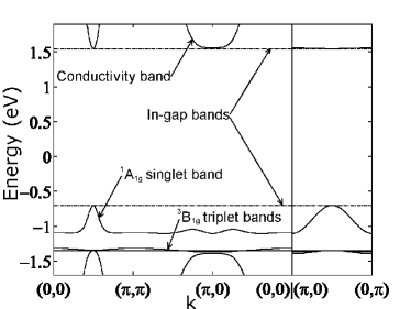
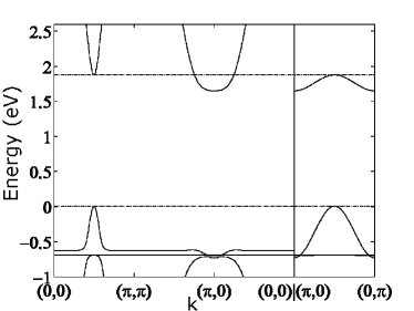
Figure 6: The AFM band structure of La₂CuO₄ obtained in the GTB method with phenomenological set of parameters (left) and in the LDA+GTB method (right). In the left figure bands are labelled; in other GTB band structure figures relative positions of bands are the same.

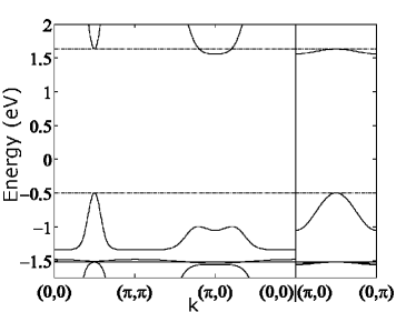
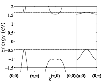
Figure 7: The AFM band structure of Nd₂CuO₄ obtained in the GTB method with phenomenological set of parameters (left) and in the LDA+GTB method (right).

The GTB band structure obtained for both phenomenological and ab initio sets of parameters is almost identical: the valence band, located below 0 eV in figures, and the conductivity band, located above +1.5 eV, divided by the insulator gap of the charge transfer origin $E_{ct}\approx 2$ eV; the undoped La₂CuO₄ and Nd₂CuO₄ are insulators in both antiferromagnetic and paramagnetic states. In-gap states at the top of the valence band and about the bottom of the conductivity band are shown by dashed lines. Their spectral weights and dispersions are proportional to doping $x$ and concentration of magnons korshunov4 . Therefore, for undoped compounds, in the Hubbard-I approximation used in GTB method, these states are dispersionless with zero spectral weight.

The valence band have bandwidth about 6 eV and consists of a set of very narrow subbands with the highest one at the top of the valence band - the so-called “Zhang-Rice singlet” subband. The dominant spectral weight in the singlet band stems from the oxygen $p$-states, while for the bottom of the empty conductivity band it is from $d_{x^{2}-y^{2}}$-states of copper. Both methods give small, less then 0.5 eV, splitting between the ${}^{1}A_{1g}$ Zhang-Rice-type singlet band and ${}^{3}B_{1g}$ narrow triplet band located below the singlet band (e.g. in the Fig. 7 for Nd₂CuO₄ it is located at -1.5 eV). The energy of Cu-$d_{3z^{2}-r^{2}}$ orbital plays the dominant role in this splitting in the GTB method. For La₂CuO₄ energy $\varepsilon_{d_{z^{2}}}$ is smaller then for Nd₂CuO₄ (see Table 3). This results in smaller width of the singlet band for the LSCO compared to the NCCO: about 0.5 eV and 1 eV correspondingly.

However, for La₂CuO₄ minor discrepancies occurs in the dispersion of the bottom of the conductivity band near $(\pi,0)$ point obtained by GTB with phenomenological set of parameters and by LDA+GTB. This leads to the different character of the optical absorption edge in two presented methods. The absorption edge for the LDA+GTB is formed by the indirect transitions in contrast to the GTB method with phenomenological set of parameters, where the momentum of excited quasiparticle is conserved by optical transition at the absorption edge. For Nd₂CuO₄ both GTB method with fitting parameters and LDA+GTB result in the conductivity band minima at the $(\pi,0)$ point (see Fig. 7). Also, in the LDA+GTB method the triplet band dispersion and the singlet-triplet hybridization are much smaller then in the GTB method with fitting parameters. This happens mainly due to the smaller values of $t^{\prime}_{pp}$ used in LDA+GTB method, because it is this microscopic parameter that gives main numerical contribution (see Eqs. (III), (IV) and (IV)) to the $t_{fg}^{TT}$ and $t_{fg}^{ST}$ - hoppings that determines the triplet band dispersion and the singlet-triplet hybridization respectively. So, despite some minor discrepancies, both GTB method with phenomenological parameters and LDA+GTB method without free parameters gives similar band dispersion.

Next topic that we will discuss in connection to the LDA+GTB method is the value of magnetic moment on copper $M_{\textrm{Cu}}$. From the neutron diffraction studies of La₂CuO₄ vaknin1 and YBa₂Cu₃O₆ tranquada1 it is known that $M_{\textrm{Cu}}$ is equal to $0.5\mu_{B}$ where $\mu_{B}$ is Bohr magneton. There are two reasons of why $M_{\textrm{Cu}}$ is different from the free atomic value $1.14\mu_{B}$ in $S=1/2$ Cu²⁺, namely zero temperature quantum spin fluctuations and the covalent effect. Since each oxygen have two neighboring coppers belonging to different magnetic sublattices the total moment on oxygen is equal to zero. But due to $p-d$ hybridization the $p$-states of oxygen are partially filled so these orbitals could carry non-zero magnetic moment $M_{\textrm{O}}$, while total moment on oxygen will be equal to zero. Such space distribution of magnetic moment leads to the difference freltoft1 between experimentally observed antiferromagnetic form-factor for La₂CuO₄ and the Heisenberg form-factor of Cu²⁺. In order to take into account covalent effects and zero quantum fluctuations on equal footing we will write down the expression for $M_{\textrm{Cu}}$:

$$M_{\textrm{Cu}}=2.28\mu_{B}\left<S^{z}\right>u^{2},$$ (24)

where zero quantum spin fluctuations are contained in $\left<S^{z}\right>$ and covalent effects are described by the weight $u^{2}$ of the $d^{9}p^{6}$ configuration. The last quantity is calculated in the framework of the LDA+GTB method and equal to $u^{2}=0.5$. In paper horsch1, the value $\left<S^{z}\right>=0.3$ was obtained self-consistently in the effective quasi-two-dimensional Heisenberg antiferromagnetic model for typical in $La_{2}CuO_{4}$ ratio $10^{-5}$ of the interplane and intraplane exchange parameters. Close value of $\left<S^{z}\right>=0.319$ was obtained in Ref. katanin1, where also the plaquette ring-exchange was considered in Heisenberg Hamiltonian. Using Eq. (24) and above values of $u^{2}$ and $\left<S^{z}\right>$ we have calculated magnetic moment on copper $M_{\textrm{Cu}}=0.4\mu_{B}$, that is close to the experimentally observed $M_{\textrm{Cu}}=0.5\mu_{B}$.

Summarizing this section, we can conclude that the proposed LDA+GTB scheme works quite well and could be used for quantitative description of the High-$T_{c}$ cuprates. The LDA+GTB scheme also can be used for wide class of SCES - cuprates, manganites, and other.

V Effective low-energy model

When we are interested in the low-energy physics (like e.g. superconductivity) it is useful to reduce the microscopic model to more simpler effective Hamiltonian. For example, for the Hubbard model in the regime of strong correlations the effective model is the $t-J$* model ($t-J$ model plus 3-centers correlated hoppings $H_{3}$) obtained by exclusion of the intersubband hoppings perturbatively. bulaevskii1 ; chao1 ; hirsch1 Analysis of the 3-band model results in the effective Hubbard and the $t-J$ model. rice1 ; lovtsov1 ; schutler1 ; belinicher1 ; feiner1

As the next step we will formulate the effective model for the multiband $p-d$ model. Simplest way to do it is to neglect completely contribution of two-particle triplet state ${}^{3}B_{1g}$. Then there will be only one low-energy two-particle state – Zhang-Rice-type singlet ${}^{1}A_{1g}$ – and the effective model will be the usual $t-J$* model. But in the multiband $p-d$ model the difference $\epsilon_{T}-\epsilon_{S}$ between energy of two-particle singlet and two-particle triplet depends strongly on various model parameters, particularly on distance of the apical oxygen from the planar oxygen, energy of the apical oxygen, difference between energy of $d_{z^{2}}$-orbitals and $d_{x^{2}}$-orbitals. For the realistic values of model parameters $\varepsilon_{T}-\varepsilon_{S}$ is close to $0.5$ eV gavrichkov2 ; raimondi1 contrary to the 3-band model with this value being about $2$ eV. To take into account triplet states we will derive the effective Hamiltonian for multiband $p-d$ model by exclusion of the intersubband hopping between low (LHB) and upper (UHB) Hubbard subbands. These subbands divided by the energy of charge-transfer gap $E_{ct}\approx 2$ eV (similar to $U$ in the Hubbard model) and using perturbation theory, similar to Ref. chao1, , with small parameter $W/U$ we can derive separate effective models for UHB and LHB. This procedure is schematically shown in Fig. 5. And, as one can see, since the UHB and LHB in initial model (III) are formed by different quasiparticles (namely, $\alpha_{0}$ for LHB and $\alpha_{1}$, $\alpha_{2}$, $\alpha_{3}$ for UHB in Fig. 5), the effective models will be different for upper (valence band, hole doped) and lower (conductivity band, electron doped) subbands.

We write the Hamiltonian in the form $H=H_{0}+H_{1}$, where the excitations via the charge transfer gap $E_{ct}$ are included in $H_{1}$. Then we define an operator $H(\epsilon)=H_{0}+\epsilon H_{1}$ and make the unitary transformation $\tilde{H}(\epsilon)=\exp{(-i\epsilon\hat{S})}H\left(\epsilon\right)\exp{(i\epsilon\hat{S})}$. Vanishing linear in $\epsilon$ component of $\tilde{H}(\epsilon)$ gives the equation for matrix $\hat{S}$: $H_{1}+i\left[H_{0},\hat{S}\right]=0$. The effective Hamiltonian is obtained in second order in $\epsilon$ and at $\epsilon=1$ is given by $\tilde{H}=H_{0}+\frac{1}{2}i\left[H_{1},\hat{S}\right]$. For the multiband $p-d$ model (III) in case of electron doping we obtain the usual $t-J$* model describing conductivity band:

$$H_{t-J*} = \sum_{f,\sigma}\varepsilon_{1}X_{f}^{\sigma,\sigma}+\sum_{f\neq g,\sigma}t_{fg}^{00}X_{f}^{\sigma,0}X_{g}^{0,\sigma}+\sum\limits_{f\neq g\neq m,\sigma}H_{3}$$ (25)

$$+ \sum_{f\neq g}J_{fg}\left(\vec{S}_{f}\vec{S}_{g}-\frac{1}{4}n_{f}n_{g}\right),$$

here $H_{3}$ contains three-centers interaction terms given by Eq. (27), $\vec{S}_{f}$ are spin operators and $n_{f}$ are number of particles operators. The $J_{fg}=2\left(t_{fg}^{0S}\right)^{2}/E_{ct}$ is the exchange parameter.

For p-type systems the effective Hamiltonian has the form of the singlet-triplet $t-J$* model describing valence band:

$$H_{eff} = H_{0}+H_{t}+\sum\limits_{f\neq g\neq m,\sigma}H_{eff3}$$ (26)

$$+ \sum_{f\neq g}J_{fg}\left(\vec{S}_{f}\vec{S}_{g}-\frac{1}{4}n_{f}n_{g}\right).$$

Three-centers interaction terms $H_{eff3}$ are given by Eq. (28). Expressions for $H_{0}$ and $H_{t}$ are as the follows:

$$H_{0} = \sum_{f}\left[\varepsilon_{1}\sum_{\sigma}X_{f}^{\sigma,\sigma}+\varepsilon_{2S}X_{f}^{S,S}+\varepsilon_{2T}\sum_{M}X_{f}^{TM,TM}\right],$$

$$H_{t} = \sum_{f\neq g,\sigma}\Bigl{\{}t_{fg}^{SS}X_{f}^{S,\bar{\sigma}}X_{g}^{\bar{\sigma},S}$$

$$+ t_{fg}^{TT}\left(\sigma\sqrt{2}X_{f}^{T0,\bar{\sigma}}-X_{f}^{T2\sigma,\sigma}\right)\left(\sigma\sqrt{2}X_{g}^{\bar{\sigma},T0}-X_{g}^{\sigma,T2\sigma}\right)$$

$$+ t_{fg}^{ST}2\sigma\gamma_{b}\left[X_{f}^{S,\bar{\sigma}}\left(\sigma\sqrt{2}X_{g}^{\bar{\sigma},T0}-X_{g}^{\sigma,T2\sigma}\right)+h.c.\right]\Bigl{\}}.$$

The resulting Hamiltonian (26) is the two-band generalization of the $t-J$* model. Significant feature of effective singlet-triplet model is the asymmetry for n- and p-type systems which is known experimentally. So, we can conclude that for n-type systems the usual $t-J$* model takes place while for p-type superconductors with complicated structure on the top of the valence band the singlet-triplet transitions are important.

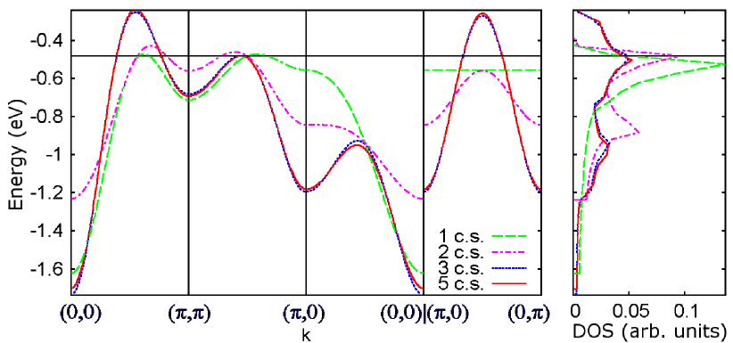
Figure 8: (Color online) Quasiparticle dispersion and corresponding densities of states (DOS) in the $t-J$* model calculated for different number of taken into account coordination spheres (c.s.). Chemical potential shown by the straight horizontal line was calculated self-consistently assuming 15% holes doping.

Contrary to the multiband $p-d$ model’s parameters that fall with distance rapidly, effective model parameters do not decrease so fast. This happens due to weak distance dependence of Wannier functions that determine coefficients $\mu_{fg}$, $\nu_{fg}$, $\lambda_{fg}$, $\xi_{fg}$, $\chi_{fg}$ gavrichkov1 which, in turn, determine distance dependence of effective model parameters (III).

To demonstrate the importance of hoppings to far coordination spheres (c.s.) in the Fig. 8 we present the dispersion and DOS in the $t-J$* model with parameters from Table 4. The electron Green function (19) has been calculated beyond the Hubbard-I approximation by a decoupling of static correlation functions that includes short-range magnetic order: $\left<X_{f}^{\sigma\sigma}X_{g}^{\sigma^{\prime}\sigma^{\prime}}\right>\to n_{p}^{2}+\frac{\sigma}{\sigma^{\prime}}\frac{1}{2}C_{fg}$, $\left<X_{f}^{\sigma\bar{\sigma}}X_{g}^{\bar{\sigma}\sigma}\right>=C_{fg}$. Here $n_{p}$ is the occupation factors of the single-particle state, $C_{fg}=2\left<S_{f}^{z}S_{g}^{z}\right>$ are static spin correlation functions which were self-consistently calculated from the spin Green’s functions in the 2D $t-J$ model. sherman1 As one can easily see from Fig. 8, the dispersion with hoppings only to nearest neighbors (1 c.s.) and to next-nearest neighbors (2 c.s., the so called $t-t^{\prime}-J$* model) is quantitatively different around $(0,0)$ point and qualitatively different around $(\pi,0)$ point from the dispersion with 3 c.s. ($t-t^{\prime}-t^{\prime\prime}-J$* model) and more coordination spheres taken into account.

Recent ARPES experimentszhou1 show that the Fermi velocity $v_{F}=E_{F}/k_{F}$ is nearly constant for wide range of p-type materials and doping independent within an experimental error of 20%. We have calculated this quantity in the $t-J$* model with parameters from Table 4 in the approximation described above. In the doping range from $x=0.03$ to $x=0.15$ our calculations give very weak doping dependence of the Fermi velocity. Assuming the lattice constant equal to 4Å we have $v_{F}$ varying from $1.6$ eVÅ^-1 to $2.0$ eVÅ^-1. Taking into account experimental error of 20% our results is very close to the experimental one.

VI Conclusion

The approach developed here assumes the multiband Hamiltonian for the real crystal structure and its mapping onto low-energy model. Parameters of the effective model (III) are obtained directly from ab initio multiband model parameters. The sets of parameters for the effective models (25) and (26) are presented in Tables 4 and 5 for p- and n-type cuprates, correspondingly.

The effective low-energy model appears to be the $t-t^{\prime}-t^{\prime\prime}-J$* model (25) for Nd₂CuO₄ and the singlet-triplet $t-t^{\prime}-t^{\prime\prime}-J$* model (26) for La₂CuO₄. There is almost no difference in the band dispersion with addition of numerically small hoppings to 4-th, 5-th, etc. neighbors.

Summarizing, we have shown that the hybrid LDA+GTB method incorporate the ab initio calculated parameters of the multiband $p-d$ model and the adequate treatment of strong electron correlations.

*

Appendix A Expressions for 3-centers Correlated Hoppings in Effective Models

In the $t-J$* model (25) the 3-centers correlated hoppings are given by:

$$H_{3}={\frac{{t_{fm}^{0S}t_{mg}^{0S}}}{{E_{ct}}}\left(X_{f}^{\sigma 0}X_{m}^{\bar{\sigma}\sigma}X_{g}^{0\bar{\sigma}}-X_{f}^{\sigma 0}X_{m}^{\bar{\sigma}\bar{\sigma}}X_{g}^{0\sigma}\right)}.$$ (27)

The three-centers interaction terms $H_{eff3}$ in the effective Hamiltonian (26) are much more complicated then in the $t-J$* model due to additional triplet and singlet-triplet contributions:

$$H_{eff3}={\frac{{t_{fm}^{0S}t_{mg}^{0S}}}{{E_{ct}}}H_{3}^{SS}-v\frac{{t_{fm}^{0S}t_{mg}^{ST}}}{{E_{ct}}}H_{3}^{ST}+v^{2}\frac{{t_{fm}^{ST}t_{mg}^{ST}}}{{E_{ct}}}H_{3}^{TT}},$$ (28)

$$H_{3}^{SS}=\left({X_{f}^{\sigma S}X_{m}^{\bar{\sigma}\sigma}X_{g}^{S\bar{\sigma}}-X_{f}^{\bar{\sigma}S}X_{m}^{\sigma\sigma}X_{g}^{S\bar{\sigma}}}\right),$$

$$H_{3}^{ST} = \frac{1}{{\sqrt{2}}}\left({X_{f}^{\sigma T0}X_{m}^{\bar{\sigma}\sigma}X_{g}^{S\bar{\sigma}}-X_{f}^{\bar{\sigma}T0}X_{m}^{\sigma\sigma}X_{g}^{S\bar{\sigma}}}\right)$$

$$+ 2\sigma\left({X_{f}^{\bar{\sigma}T2\bar{\sigma}}X_{m}^{\bar{\sigma}\sigma}X_{g}^{S\bar{\sigma}}+X_{f}^{\sigma T2\sigma}X_{m}^{\sigma\sigma}X_{g}^{S\bar{\sigma}}}\right)$$

$$+ \frac{1}{{\sqrt{2}}}\left({X_{f}^{\sigma S}X_{m}^{\bar{\sigma}\sigma}X_{g}^{T0\bar{\sigma}}-X_{f}^{\bar{\sigma}S}X_{m}^{\sigma\sigma}X_{g}^{T0\bar{\sigma}}}\right)$$

$$- 2\sigma\left({X_{f}^{\sigma S}X_{m}^{\bar{\sigma}\sigma}X_{g}^{T2\sigma\sigma}-X_{f}^{\bar{\sigma}S}X_{m}^{\sigma\sigma}X_{g}^{T2\sigma\sigma}}\right),$$

$$H_{3}^{TT} = \frac{1}{2}\left({X_{f}^{\sigma T0}X_{m}^{\bar{\sigma}\sigma}X_{g}^{T0\bar{\sigma}}-X_{f}^{\bar{\sigma}T0}X_{m}^{\sigma\sigma}X_{g}^{T0\bar{\sigma}}}\right)$$

$$- \left({X_{f}^{\bar{\sigma}T2\bar{\sigma}}X_{m}^{\bar{\sigma}\sigma}X_{g}^{T2\sigma\sigma}+X_{f}^{\sigma T2\sigma}X_{m}^{\sigma\sigma}X_{g}^{T2\sigma\sigma}}\right)$$

$$+ \frac{{2\sigma}}{{\sqrt{2}}}\left({-X_{f}^{\sigma T0}X_{m}^{\bar{\sigma}\sigma}X_{g}^{T2\sigma\sigma}+X_{f}^{\bar{\sigma}T0}X_{m}^{\sigma\sigma}X_{g}^{T2\sigma\sigma}}\right)$$

$$+ \frac{{2\sigma}}{{\sqrt{2}}}\left({+X_{f}^{\bar{\sigma}T2\bar{\sigma}}X_{m}^{\bar{\sigma}\sigma}X_{g}^{T0\bar{\sigma}}+X_{f}^{\sigma T2\sigma}X_{m}^{\sigma\sigma}X_{g}^{T0\bar{\sigma}}}\right).$$

References

- (1) P. Hohenberg and W. Kohn, Phys. Rev. 136, 864 (1964).
- (2) W. Kohn and L.J. Sham, Phys. Rev. 140, 1133 (1965).
- (3) V.I. Anisimov, J. Zaanen, and O.K. Andersen, Phys. Rev. B 44, 943 (1991).
- (4) A. Svane and O. Gunnarsson, Phys. Rev. Lett. 65, 1148 (1990).
- (5) J.C. Hubbard, Proc. Roy. Soc. A 276, 238 (1963).
- (6) V.I. Anisimov, A.I. Poteryaev, M.A. Korotin, A.O. Anokhin, and G. Kotliar, J. Phys.: Condens. Matter 35, 7359 (1997).
- (7) K. Held, I.A. Nekrasov, N. Blümer, V.I. Anisimov, and D. Vollhardt, Int. J. Mod. Phys. B 15, 2611 (2001); K. Held, I.A. Nekrasov, G. Keller, V. Eyert, N. Blümer, A.K. McMahan, R.T. Scalettar, T. Pruschke, V.I. Anisimov, and D. Vollhardt, cond-mat/0112079 (Published in Quantum Simulations of Complex Many-Body Systems: From Theory to Algorithms, eds. J. Grotendorst, D. Marks, and A. Muramatsu, NIC Series Volume 10 (NIC Directors, Forschunszentrum Jülich, 2002) p. 175-209. (ISBN 3-00-009057-6)
- (8) K. Held, I.A. Nekrasov, G. Keller, V. Eyert, N. Blümer, A.K. McMahan, R.T. Scalettar, Th. Pruschke, V.I. Anisimov, and D. Vollhardt, “Realistic investigations of correlated electron systems with LDA+DMFT”, Psi-k Newsletter 56 (April 2003), p. 65-103 [psi-k.dl.ac.uk/newsletters/News_56/Highlight_56.pdf].
- (9) A.I. Lichtenstein and M.I. Katsnelson, Phys. Rev. B 57, 6884 (1998).
- (10) D. Vollhardt, in Correlated Electron Systems, edited by V. J. Emery, World Scientific, Singapore, 1993, p. 57.
- (11) G. Kotliar and D. Vollhardt, Physics Today 57, No. 3 (March), 53 (2004).
- (12) W. Metzner and D. Vollhardt, Phys. Rev. Lett. 62, 324 (1989).
- (13) A. Georges, G. Kotliar, W. Krauth, and M. Rozenberg, Rev. Mod. Phys. 68, 13 (1996).
- (14) M.H. Hettler, A.N. Tahvildar-Zadeh, M. Jarrell, T. Pruschke, and H.R. Krishnamurthy, Phys. Rev. B 58, R7475 (1998).
- (15) Th. Maier, M. Jarrell, Th. Pruschke and M. Hettler, Rev. Mod. Phys. (in print, cond-mat/0404055 (2004)).
- (16) S.Yu. Savrasov and G. Kotliar, Phys. Rev. B 69, 245101 (2004).
- (17) S.G. Ovchinnikov and I.S. Sandalov, Physica C 161, 607 (1989).
- (18) V.J. Emery, Phys. Rev. Lett. 58, 2794 (1987).
- (19) C.M. Varma, S. Smitt-Rink, and E. Abrahams, Solid State Commun. 62, 681 (1987).
- (20) S.V. Lovtsov and V.Yu. Yushankhai, Physica C 179, 159 (1991).
- (21) J.H. Jefferson, H. Eskes, and L.F. Feiner, Phys. Rev. B 45, 7959 (1992).
- (22) H-B. Schu̧ttler and A.J. Fedro, Phys. Rev. B 45, R7588 (1992).
- (23) V.A. Gavrichkov, S.G. Ovchinnikov, A.A. Borisov, and E.G. Goryachev, Zh. Eksp. Teor. Fiz. 118, 422 (2000); [JETP 91, 369 (2000)].
- (24) V. Gavrichkov, A. Borisov, and S.G. Ovchinnikov, Phys. Rev. B 64, 235124 (2001).
- (25) V.A. Gavrichkov, S.G. Ovchinnikov, and L.E. Yakimov, submitted to JETP (2005).
- (26) S.G. Ovchinnikov and O.G. Petrakovsky, J. Superconductivity 4, 437 (1991).
- (27) G.H. Wannier, Phys. Rev. 52, 191 (1937).
- (28) N. Marzari and D. Vanderbilt, Phys. Rev. B 56, 12847 (1997).
- (29) Wei Ku, H. Rosner, W.E. Pickett, and R.T. Scalettar, Phys. Rev. Lett. 89, 167204 (2002).
- (30) O.K. Andersen and O. Jepsen, Phys. Rev. Lett. 53, 2571 (1984).
- (31) V.I. Anisimov, D.E. Kondakov, A.V. Kozhevnikov, I.A. Nekrasov, Z.V. Pchelkina, J.W. Allen, S.-K. Mo, H.-D. Kim, P. Metcalf, S. Suga, A. Sekiyama, G. Keller, I. Leonov, X. Ren, and D. Vollhardt, Phys. Rev. B 71, 125119 (2005).
- (32) O.K. Andersen, Z. Pawlowska, and O. Jepsen, Phys.Rev. B 34, 5253 (1986).
- (33) P.G. Radaelli, D.G. Hinks, A.W. Mitchell, B.A. Hunter, J.L. Wagner, B. Dabrowski, K.G. Vandervoort, and H.K. Viswanathan, J.D. Jorgensen, Phys. Rev. B. 49, 4163 (1994).
- (34) T. Kamiyama, F. Izumi, H. Takahashi, J.D. Jorgensen, B. Dabrowski, R.L. Hitterman, D.G. Hinks, H. Shaked, T.O. Mason, and M. Seabaugh, Physica C 229, 377-388 (1994).
- (35) O. Gunnarsson, O.K. Andersen, O. Jepsen, and J. Zaanen, Phys. Rev. B. 39, 1708 (1989); V.I. Anisimov and O. Gunnarsson, 43, 7570 (1991).
- (36) V.I. Anisimov, M.A. Korotin, I.A. Nekrasov, Z.V. Pchelkina, and S. Sorella, Phys. Rev. B. 66, 100502(R) (2002).
- (37) Yu. Gaididei and V. Loktev, Phys. Status Solidi B 147, 307 (1988).
- (38) A. Bianconi, M. De Santis, and A. Di Cicco, A.M. Flank, A. Fontaine, and P. Lagarde, H. Katayama-Yoshida and A. Kotani, A. Marcelli, Phys. Rev. B 38, R7196 (1988).
- (39) H. Romberg, N. Nücker, M. Alexander, and J. Fink, D. Hahn, T. Zetterer, H.H. Otto, and K.F. Renk, Phys. Rev. B 41, R2609 (1990).
- (40) C.T. Chen, L.H. Tjeng, J. Kwo, H.L. Kao, P. Rudolf, F. Sette, and R.M. Fleming, Phys. Rev. Lett. 68, 2543 (1992).
- (41) R. Raimondi and J.H. Jefferson, L.F. Feiner, Phys. Rev. B 53, 8774 (1996).
- (42) J.C. Hubbard, Proc. Roy. Soc. London A 277, 237 (1964).
- (43) M.M. Korshunov, V.A. Gavrichkov, S.G. Ovchinnikov, Z.V. Pchelkina, I.A. Nekrasov, M.A. Korotin, and V.I. Anisimov, Zh. Eksp. Teor. Fiz. 126, 642 (2004) [JETP 99, 559 (2004)].
- (44) M.M. Korshunov, V.A. Gavrichkov, S.G. Ovchinnikov, D. Manske, and I. Eremin, Physica C 402, 365 (2004).
- (45) B.O. Wells, Z.-X. Shen, A. Matsuura, D.M. King, M.A. Kastner, M. Greven, and R. J. Birgeneau, Phys. Rev. Lett. 74, 964 (1995).
- (46) C. Dürr, S. Legner, R. Hayn, S.V. Borisenko, Z. Hu, A. Theresiak, M. Knupfer, M.S. Golden, J. Fink, F. Ronning, Z.-X. Shen, H. Eisaki, S. Uchida, C. Janowitz, R. Müller, R.L. Johnson, K. Rossnagel, L. Kipp, and G. Reichardt, Phys. Rev. B 63, 014505 (2000).
- (47) A.A. Borisov, V.A. Gavrichkov, and S.G. Ovchinnikov, Mod. Phys. Lett. B 17, 479 (2003).
- (48) A.A. Borisov, V.A. Gavrichkov, and S.G. Ovchinnikov, Zh. Eksp. Teor. Fiz. 124, 862 (2003); [JETP 97, 773 (2003)].
- (49) A. Ino, T. Mizokawa, and A. Fujimori, K. Tamasaku, H. Eisaki, S. Uchida, T. Kimura, T. Sasagawa, and K. Kishio, Phys. Rev. Lett. 79, 2101 (1997).
- (50) N. Harima, J. Matsuno, and A. Fujimori, Y. Onose, Y. Taguchi, and Y. Tokura, Phys. Rev B 64, 220507(R) (2001).
- (51) A. Ino, C. Kim, M. Nakamura, T. Yoshida, T. Mizokawa, A. Fujimori, Z.-X. Shen, T. Kakeshita, H. Eisaki, and S. Uchida, Phys. Rev. B 65, 094504 (2002).
- (52) N.P. Armitage, D.H. Lu, C. Kim, A. Damascelli, K.M. Shen, F. Ronning, D.L. Feng, P. Bogdanov, and Z.-X. Shen, Y. Onose, Y. Taguchi, and Y. Tokura, P.K. Mang, N. Kaneko, and M. Greven, Phys. Rev. Lett. 87, 147003 (2001).
- (53) R.O. Zaitsev, Sov. Phys. JETP 41, 100 (1975).
- (54) Yu.A. Izumov and B.M. Letfullov, J. Phys.: Condens. Matter 3, 5373 (1991).
- (55) S.G. Ovchinnikov and V.V. Val’kov, Hubbard Operators in the Theory of Strongly Correlated Electrons (Imperial College Press, London-Singapore, 2004).
- (56) V.G. Bar’yakhtar, V.N. Krivoruchko, and D.A.Yablonskii, Green’s Functions in Magnetism Theory [in Russian], (Nauk. Dumka, Kiev, 1984).
- (57) O.K. Andersen, A.I. Liechtenstein, O. Jepsen, and F. Paulsen, J. Phys. Chem. Solids 56, 1573 (1995).
- (58) E. Pavarini, I. Dasgupta, T. Saha-Dasgupta, O. Jepsen, and O.K. Andersen, Phys. Rev. Lett. 87, 047003 (2001).
- (59) A.S. Moskvin, J. Ma’lek, M. Knupfer, R. Neudert, J. Fink, R. Hayn, S.-L. Drechsler, N. Motoyama, H. Eisaki, and S. Uchida, Phys. Rev. Lett. 91, 037001 (2003).
- (60) A.S. Moskvin, Pis’ma v ZhETF 80, 824 (2004) [JETP Lett. 80, 697 (2004)].
- (61) T. Tohyama and S. Maekawa, Phys. Rev. B 49, 3596 (1994).
- (62) S.G. Ovchinnikov, A.A. Borisov, V.A. Gavrichkov, and M.M. Korshunov, J. Phys.: Condens. Matter 16, L93 (2004).
- (63) D. Vaknin, S. K. Sinha, D. E. Moncton, D. C. Johnston, J. M. Newsam, C. R. Safinya, and H. E. King, Jr., Phys. Rev. Lett. 58, 2802 (1987).
- (64) J.M. Tranquada, A.H. Moudden, A.I. Goldman, P. Zolliker, D.E. Cox, and G. Shirane, S.K. Sinha, D. Vaknin, D.C. Johnston, M. S. Alvarez, A.J. Jacobson, J.T. Lewandowski, and J.M. Newsam , Phys. Rev. B 38, 2477 (1988).
- (65) T. Freltoft and G. Shirane, S. Mitsuda, J.P. Remeika and A.S. Cooper, Phys. Rev. B 37, 137 (1988).
- (66) P. Horsch and W. von der Linden, Z. Phys. B: Condens. Matter 72, 181 (1988).
- (67) A.A. Katanin and A.P. Kampf, Phys. Rev. B 66, 100403(R) (2003).
- (68) L.N. Bulaevskii, E.L. Nagaev, D.I. Khomskii, Sov. Phys. JETP 54, 1562 (1968).
- (69) K.A. Chao, J. Spalek and A.M. Oles, J. Phys. C: Sol. Stat. Phys. 10, 271 (1977).
- (70) J.E. Hirsch, Phys. Rev. Lett. 54, 1317 (1985).
- (71) F.C. Zhang and T.M. Rice, Phys. Rev. B 41, 7243 (1990).
- (72) V.I. Belinicher and A.L. Chernyshev, Phys. Rev. B 47, 390 (1993).
- (73) L.F. Feiner, J.H. Jefferson, and R. Raimondi, Phys. Rev. B 53, 8751 (1996).
- (74) A. Sherman and M. Schreiber, Eur. Phys. J. B 32, 203 (2003).
- (75) X.J. Zhou, T. Yoshida, A. Lanzara, P.V. Bogdanov, S.A. Kellar, K.M. Shen, W.L. Yang, F. Ronning, T. Sasagawa, T. Kakeshita, T. Noda, H. Eisaki, S. Uchida, C.T. Lin, F. Zhou, J.W. Xiong, W.X. Ti, Z.X. Zhao, A. Fujimori, Z. Hussain and Z.-X. Shen, Nature 423, 398 (2003).