Theory of thermal and charge transport in diffusive normal metal / superconductor junctions

Abstract

Thermal and charge transport in diffusive normal metal(DN) / insulator / $s$-, $d$- and $p$-wave superconductor junctions are studied based on the Usadel equation with the Nazarov’s generalized boundary condition. We derive a general expression of the thermal conductance in unconventional superconducting junctions. Thermal conductance, electric conductance of junctions and their Lorentz ratio are calculated as a function of resistance in DN, the Thouless energy, magnetic scattering rate in DN and transparency of the insulating barrier. We also discuss transport properties for various orientation angles between the normal to the interface and the crystal axis of superconductors. It is demonstrated that the proximity effect does not influence the thermal conductance while the midgap Andreev resonant states suppress it. Dependencies of the electrical and thermal conductance on temperature are sensitive to pairing symmetries and orientation angles. The results imply a possibility to distinguish one pairing symmetry from another based on the results of experimental observations.

I Introduction

Thermal and electrical conductances are basic properties of a metal. The abilities to carry heat and charge currents are related to each other. At low temperatures thermal conductivity $\kappa$ of a metal is linear in $T$, i.e., $\kappa\propto T$, while the electrical conductivity $\sigma$ approaches a constant. As a result, the Lorentz ratio becomes a universal constant: $L\equiv\kappa/\sigma T=\pi^{2}/3e^{2}$. This characteristic feature is called the Wiedemann-Franz (WF) law WF and has been observed in various electron systems Kearney ; Castellani ; Chester ; Smrcka ; Ong which may be described by the Fermi liquid theory. A violation of the WF law implies the breakdown of the Fermi liquid description of the electronic states in a metal. For instance, in the normal state of high-T_c cuprates the violation of the WF law suggests the non-Fermi liquid description Hill . A validity of the Fermi liquid picture in cuprates is an open question even now.

The heat and charge currents are also important characteristics of a superconducting state. Thermal conductivity of a bulk superconductor was first discussed theoretically by Bardeen et al. Badeen . Large amount of work was done on thermal and electric transport in contacts between normal and superconducting phases (N/S junctions). In the pioneering work by Andreev Andreev a new type of quasiparticle scattering at the N/S interface was discovered, the so-called Andreev reflection (AR), which crucially influences quasiparticle transport across the interface at subgap energies. The AR causes the exponential decay of a thermal conductance across the N/S interface with decreasing temperature Andreev , while it facilitates the transfer of an electric charge BTK . As shown by Blonder, Tinkham and Klapwijk (BTK) BTK , the AR leads to the doubling of zero bias conductance across transparent N/S interface at low $T$. More recently, Bardas and AverinBardas and Devyatov et al. Devyatov calculated heat current by generalizing the BTK model BTK for the electric transport in N/S junctions. The applicability of these theories is, however, limited to junctions in the clean limit.

In most of practical N/S junctions normal metals are in the diffusive regime. Therefore the effect of impurity scattering on the transport properties has received a lot of attention. In diffusive normal metal / superconductor (DN/S) junctions, the diffusive motion of quasiparticles at a mesoscopic length scale around the interface strongly modifies the transport across a junction interface because of interference effects Hekking . For example, the appearance of the zero bias conductance peak (ZBCP) in DN/S junctions is a direct consequence of the interference effect of a quasiparticle in DN Giazotto ; Klapwijk ; Kastalsky ; Nguyen ; Wees ; Nitta ; Bakker ; Xiong ; Magnee ; Kutch ; Poirier . To study such interference effects, the quasiclassical Green’s function theory Eilenberger ; Eliashberg ; Larkin has been widely used because of its convenience and broad applicability. Based on this formalism, theory of charge transport in DN/S junctions was formulated by Volkov, Zaitsev and Klapwijk (VZK) Volkov . By applying the VZK theory, a number of authors investigated theoretically charge transport in various proximity structures Lambert1 ; Nazarov1 ; Yip ; Stoof ; Reentrance ; Golubov ; Takayanagi ; Seviour ; Belzig ; Yip2 ; Yoko ; Volkov . This work was based on the boundary conditions for the Keldysh-Nambu Green’s function at the DN/S interface derived by Kupriyanov and Lukichev (KL) KL from Zaitsev’s boundary condition Zaitsev in the isotropic limit. The KL boundary conditions were recently extended by Nazarov within the circuit theory Nazarov2 and applied by Tanaka et al. TGK to the study of charge transport in N/S junctions with arbitrary interface transparency in order to investigate more complex structures. The Nazarov’s boundary conditions coincide with the KL boundary conditions when transmission coefficients are sufficiently low, while the BTK theory BTK is reproduced in the ballistic regime. It was shown in TGK that a zero bias conductance peak (ZBCP) in low transparent N/S junctions transforms to a zero bias conductance dip (ZBCD) with increasing the interface transparency.

Heat transport within the quasiclassical approach was studied by several authors Raimondi ; Beyer ; Graf ; Graf2 ; Bezuglyi . In particular, Graf et al. Graf calculated thermal conductivity for various unconventional superconductors. They showed that thermal conductivity of a clean two-dimensional $d_{x^{2}-y^{2}}$-wave superconductor is proportional to $T$ in the Born limit over a broad temperature range and proportional to $T^{3}$ in the unitary limit above some crossover temperature $T^{\ast}\sim\gamma$, where $\gamma$ is the bandwidth of quasiparticle states bound to impurities. These results also suggest that thermal conductivity is sensitive to a pairing symmetry of an unconventional superconductor Graf2 . On the other hand, heat transport in N/S junctions has not received much attention so far, partially due to the lack of experimental data. Recently, sufficient progress was achieved which made it possible to study heat transport in unconventional superconductors Movshovich ; Movshovich2 ; May ; Izawa ; Izawa2 ; Izawa3 ; Izawa4 ; Suzuki and this stimulated theoretical study of these phenomena.

The formation of the midgap Andreev resonant state (MARS) drastically affects low energy transport in unconventional superconducting junctions Buch ; TK95 ; Kashi00 ; Yamashiro ; Maeno . It is now widely accepted that MARS is also responsible for ZBCP in N/S junctions of unconventional superconductors. To discuss interplay between the proximity effect and MARS, a new circuit theory for unconventional superconductors was proposed in Nazarov2003 ; TNGK ; p-wave . In DN/$d$-wave superconductor junctions, MARS interfere destructively with the proximity effect in DN Nazarov2003 ; TNGK . On the other hand, in DN/$p$-wave superconductor junctions the MARS and the proximity effect coexist p-wave . As a result, the conductance spectrum has a giant ZBCP and the local density of states in DN has a zero energy peak. We summarize relations between the proximity effect and the MARS in Fig. 1.

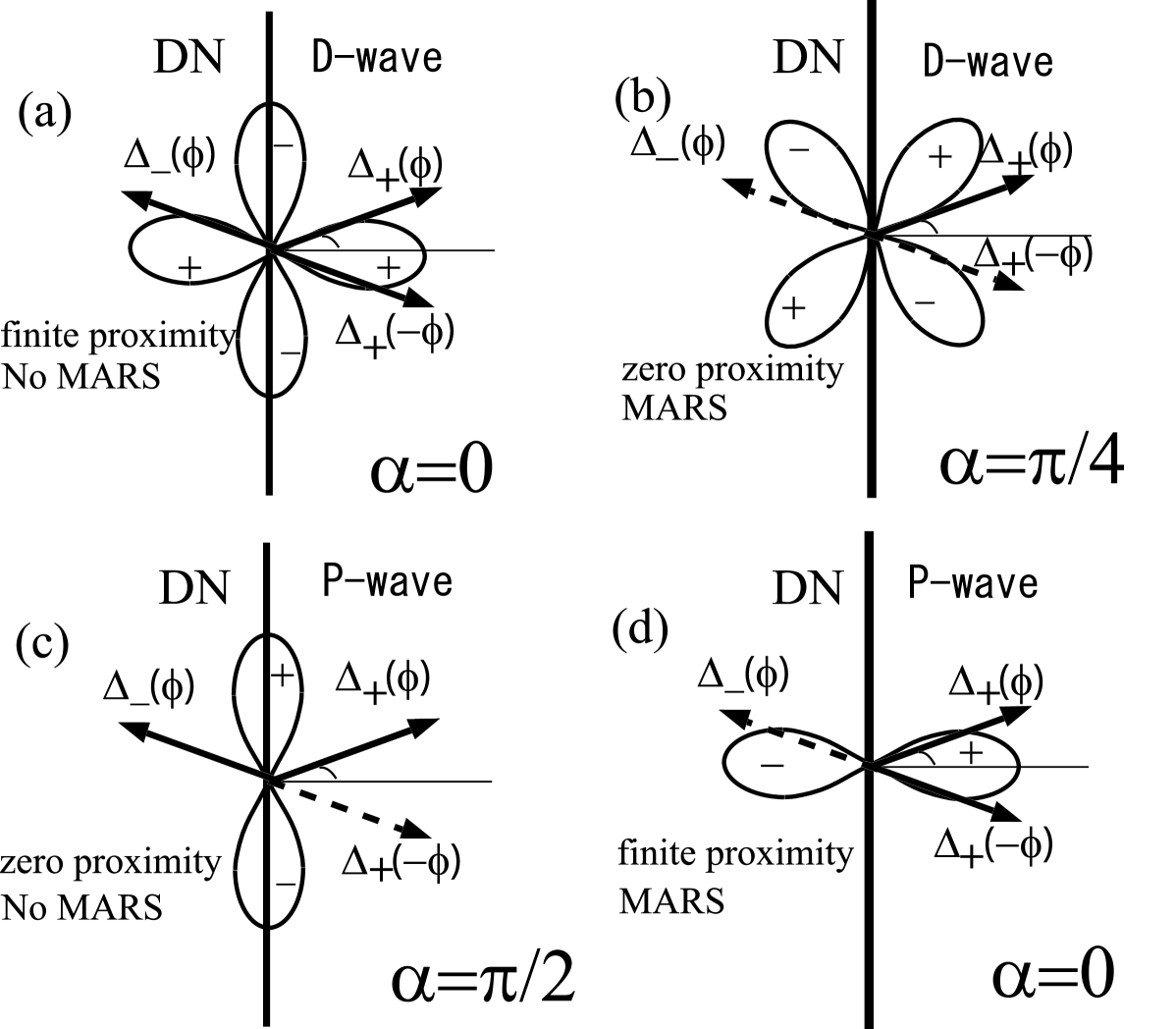
Figure 1: Schematic illustration of trajectories of incoming and outgoing quasiparticles at a DN/S interface with pair potential $\Delta_{\pm}(\phi)$. The pair potentials $\Delta_{\pm}$ are given by $\Delta_{\pm}=\Delta(T)\cos[2(\phi\mp\alpha)]$ for $d$-wave superconductors (D-wave) where $\alpha$ denotes the angle between the normal to the interface and the crystal axis of $d$-wave superconductors. For $p$-wave superconductors (P-wave) the pair potentials $\Delta_{\pm}$ are given by $\Delta_{\pm}=\pm\Delta(T)\cos[(\phi\mp\alpha)]$, where $\alpha$ denotes the angle between the normal to the interface and the lobe direction of the $p$-wave pair potential. In the above, $\phi$ denotes the injection angle of the quasiparticle measured from the $x$-axis and $\Delta(T)$ is the maximum amplitude of the pair potential at a temperature $T$.

The junctions in Fig. 1 are classified into four groups: (a) presence of the proximity effect, (b) presence of MARS, (c) absence of both MARS and the proximity effect, and (d) presence of both of them. Thermal and charge transport in N/S junctions can be described in terms of MARS and the proximity effect.

The purpose of the present paper is to study the tunneling conductance, the thermal conductance and their Lorentz ratio in diffusive normal metal / insulator / $s$-, $d$- and $p$-wave superconductor junctions as a function of transparencies of insulating barriers at the interface, resistance $R_{d}$ in DN, the magnetic scattering rate in DN, the Thouless energy $E_{Th}$ in DN, and orientation angles between the normal to the interface and the crystal axis of superconductors.

The organization of this paper is as follows. In section II, we will provide the detailed derivation of the expression for the normalized thermal conductance. In section III, the results of calculations are presented for various types of junctions. They are applied to discriminate various pairing states. In section IV, the summary of the obtained results is given. In the present paper, we use the units with $k_{B}=\hbar=1$.

II Formulation

In this section, we explain the model and the formalism. We consider a junction consisting of normal and superconducting reservoirs connected by a quasi-one-dimensional diffusive conductor with a length $L$ much larger than the mean free path. The interface between the DN and the S has a resistance $R_{b}$ while the DN/N interface has zero resistance. The positions of the DN/N interface and the DN/S interface are denoted as $x=0$ and $x=L$, respectively. According to the circuit theory, the interface between DN and S is subdivided into two isotropization zones in DN and S, two ballistic zones and a scattering zone. The sizes of the ballistic and scattering zones in the current direction are much shorter than the coherence length. The scattering zone is modeled as an infinitely narrow insulating barrier described by the delta function $U(x)=H\delta(x-L)$. The transparency of the interface $T_{n}$ is given by $T_{n}=4\cos^{2}\phi/(4\cos^{2}\phi+Z^{2})$, where $Z=2H/v_{F}$ is a dimensionless parameter, $\phi$ is an injection angle measured from the interface normal and $v_{F}$ is the Fermi velocity. The interface resistance $R_{b}$ is given by

$$R_{b}=R_{0}\frac{2}{\int_{-\pi/2}^{\pi/2}d\phi T_{n}\cos\phi},$$

where $R_{0}$ is the Sharvin resistance $R_{0}^{-1}=e^{2}k_{F}^{2}S_{c}/4\pi^{2}$, $k_{F}$ is the Fermi wave length, and $S_{c}$ is the constriction area.

We apply the quasiclassical Keldysh formalism in the following calculation of the tunneling and thermal conductance. The 4 $\times$ 4 Green’s functions in DN and S are denoted by $\check{G}_{1}(x)$ and $\check{G}_{2}(x)$, respectively. The spatial dependence of $\check{G}_{1}(x)$ in DN is determined by the static Usadel equation Usadel ,

$$D\frac{\partial}{\partial x}[\check{G}_{1}(x)\frac{\partial\check{G}_{1}(x)}{\partial x}]+i[\check{H}+i\check{\Sigma}_{spin},\check{G}_{1}(x)]=0$$ (1)

with the diffusion constant $D$ in DN, where $\check{H}$ is given by

$$\check{H}=\left(\begin{array}[]{cc}\hat{H}_{0}&0\\ 0&\hat{H}_{0}\end{array}\right),$$

with $\hat{H}_{0}=\epsilon\hat{\tau}_{3}$, $\check{\Sigma}_{spin}=\frac{\gamma}{2}\hat{\tau}_{3}\check{G}_{1}(x)\hat{\tau}_{3}$ is the self-energy for magnetic impurity scattering with the scattering rate $\gamma$ and $\epsilon$ is the quasiparticle energy. The directions of magnetic moments of impurities are random. The self-energy is given by averaging with respect to directions of magnetic moments. Thus in our calculation $\check{G}_{1}(x)$ is unit matrix in spin space.

The electric current is expressed using $\check{G}_{1}(x)$ as

$$I_{el}=\frac{-L}{4eR_{d}}\int_{0}^{\infty}d\epsilon\mathrm{Tr}[\hat{\tau}_{3}(\check{G}_{1}(x)\frac{\partial\check{G}_{1}(x)}{\partial x})^{K}],$$ (2)

where $(\check{G_{1}}(x)\frac{\partial\check{G_{1}}(x)}{\partial x})^{K}$ denotes the Keldysh component of $(\check{G_{1}}(x)\frac{\partial\check{G_{1}}(x)}{\partial x})$.

The thermal current is also expressed as

$$I_{th}=\frac{L}{4e^{2}R_{d}}\int_{0}^{\infty}d\epsilon\epsilon\mathrm{Tr}[(\check{G}_{1}(x)\frac{\partial\check{G}_{1}(x)}{\partial x})^{K}].$$ (3)

It is convenient to use the standard $\theta$-parametrization when function $\hat{R}_{1}(x)$ is expressed as

$$\hat{R}_{1}(x)=\hat{\tau}_{1}\sin\theta(x)\cos\psi+\hat{\tau}_{2}\sin\theta(x)\sin\psi+\hat{\tau}_{3}\cos\theta(x)$$ (4)

where $\cos\psi=0$ for singlet superconductors and $\sin\psi=0$ for triplet superconductors(see Ref. p-wave ). The parameter $\theta(x)$ is a measure of the proximity effect in DN.

Functions $\hat{A}_{1}(x)$ and $\hat{K}_{1}(x)$ are expressed as $\hat{A}_{1}(x)=-\hat{\tau}_{3}\hat{R}_{1}^{{\dagger}}(x)\hat{\tau}_{3}$ and $\hat{K}_{1}(x)=\hat{R}_{1}(x)\hat{f}_{1}(x)-\hat{f}_{1}(x)\hat{A}_{1}(x)$ with the distribution function $\hat{f}_{1}(x)$ which is given by $\hat{f}_{1}(x)=f_{l}(x)+\hat{\tau}_{3}f_{t}(x)$. From the retarded or advanced component of the Usadel equation, the spatial dependence of $\theta(x)$ is determined by the following equation

$$D\frac{\partial^{2}}{\partial x^{2}}\theta(x)+2i(\epsilon+i\gamma\cos[\theta(x)])\sin[\theta(x)]=0,$$ (5)

while from the Keldysh component we obtain

$$D\frac{\partial}{\partial x}[\frac{\partial f_{l}(x)}{\partial x}\mathrm{cos^{2}}\mathrm{Re}[\theta(x)]]=0.$$ (6)

The average over injection angles of quasiparticles at the interface is defined as

$$<B(\phi)>=\int_{-\pi/2}^{\pi/2}d\phi\cos\phi B(\phi)/\int_{-\pi/2}^{\pi/2}d\phi T(\phi)\cos\phi$$

with $T(\phi)=T_{n}$.

II.1 $s$-wave case

The Keldysh component $\hat{K}_{2}(x)$ is given by $\hat{K}_{2}(x)=\hat{R}_{2}(x)\hat{f}_{2}(x)-\hat{f}_{2}(x)\hat{A}_{2}(x)$ with the retarded component $\hat{R}_{2}(x)$, the advanced component $\hat{A}_{2}(x)$ and distribution function $\hat{f}_{2}(x)$. Here $\hat{R}_{2}(x)=g\hat{\tau}_{3}+f\hat{\tau}_{2}$ with $g=\epsilon/\sqrt{\epsilon^{2}-\Delta^{2}(T)}$ and $f=\Delta(T)/\sqrt{\Delta^{2}(T)-\epsilon^{2}}$, $\hat{A}_{2}(x)=-\hat{\tau}_{3}\hat{R}_{2}^{\dagger}(x)\hat{\tau}_{3}$ and $\hat{f}_{2}(x)=f_{S}=\mathrm{{tanh}[\epsilon/(2T)]}$ in thermal equilibrium with temperature $T$. The boundary condition for $\check{G}_{1}(x)$ at the DN/S interface is given byNazarov2 ,

$$\frac{L}{R_{d}}(\check{G}_{1}\frac{\partial\check{G}_{1}}{\partial x})_{\mid x=L_{-}}=R_{b}^{-1}<B>,$$ (7)

$$B=\frac{2T_{n}[\check{G}_{1}(L_{-}),\check{G}_{2}(L_{+})]}{4+T_{n}([\check{G}_{1}(L_{-}),\check{G}_{2}(L_{+})]_{+}-2)}.$$

For the electrical conductance, we obtain the following result at zero voltage TGK

$$\sigma_{S}(T)=\frac{1}{2T}\int_{0}^{\infty}\frac{d\epsilon}{\cosh^{2}[\frac{\epsilon}{2T}](\frac{R_{b}}{<I_{b0}>}+\frac{R_{d}}{L}\int_{0}^{L}\frac{dx}{\cosh^{2}\theta_{im}(x)})}$$ (8)

with

$$I_{b0}=\frac{T_{n}^{2}\Lambda_{1}+2T_{n}(2-T_{n})\Lambda_{2}}{2\mid(2-T_{n})+T_{n}[g\cos\theta_{L}+f\sin\theta_{L}]\mid^{2}},$$

$$\Lambda_{1}=(1+\mid\cos\theta_{L}\mid^{2}+\mid\sin\theta_{L}\mid^{2})(\mid g\mid^{2}+\mid f\mid^{2}+1)$$

$$+4\mathrm{Imag}[fg^{\ast}]\mathrm{Imag}[\cos\theta_{L}\sin\theta_{L}^{\ast}],$$ (9)

$$\Lambda_{2}=\mathrm{{Real}\{g(\cos\theta_{L}+\cos\theta_{L}^{\ast})+f(\sin\theta_{L}+\sin\theta_{L}^{\ast})\}},$$ (10)

where $\theta_{im}(x)$ and $\theta_{L}$ denote the imaginary parts of $\theta(x)$ and $\theta(L_{-})$ respectively.

Next we calculate the thermal conductance. Since DN is attached to the normal electrode at $x=0$, $\theta(0)$=0 and $f_{l}(0)=f_{l0}$ with $f_{l0}=\tanh[\epsilon/(2(T+\Delta T))]$ in thermal equilibrium at a temperature $T+\Delta T$.

The retarded part of Eq. (7) is the same as in Ref. TGK, . The Keldysh part of Eq. (7) reads

$$\frac{L}{R_{d}}(\frac{\partial f_{l}}{\partial x})\mathrm{{\cos^{2}}}\mathrm{Real}[\theta(x)]\mid_{x=L_{-}}=-\frac{<I_{b1}>(f_{l}(L_{-})-f_{S})}{R_{b}},$$ (11)

with

$$I_{b1}=\frac{T_{n}^{2}\Lambda_{1}^{{}^{\prime}}+T_{n}(2-T_{n})\Lambda_{2}^{{}^{\prime}}}{2\mid(2-T_{n})+T_{n}[g\cos\theta_{L}+f\sin\theta_{L}]\mid^{2}},$$

$$\Lambda_{1}^{{}^{\prime}}=(1+\mid\cos\theta_{L}\mid^{2}-\mid\sin\theta_{L}\mid^{2})(\mid g\mid^{2}-\mid f\mid^{2}+1)$$

$$+4\mathrm{Real}[fg^{\ast}]\mathrm{Real}[\cos\theta_{L}\sin\theta_{L}^{\ast}],$$ (12)

$$\Lambda_{2}^{{}^{\prime}}=4\mathrm{Real}[g]\mathrm{Real}[\cos\theta_{L}]-4\mathrm{Imag}[f]\mathrm{Imag}[\sin\theta_{L}].$$ (13)

Substituting the results into Eq. (3), we arrive at the final expression for the thermal current

$$I_{th}=\frac{1}{{e^{2}}}\int_{0}^{\infty}{\frac{{\epsilon\left({f_{l0}-f_{S}}\right)d\epsilon}}{{\frac{{R_{b}}}{{\left\langle{I_{b1}}\right\rangle}}+\frac{{R_{d}}}{L}\int\limits_{0}^{L}{\frac{{dx}}{{\cos^{2}{\mathop{\rm Re}\nolimits}\theta\left(x\right)}}}}}}$$ (14)

and the thermal conductance

$$\kappa=\mathop{\lim}\limits_{\Delta T\rightarrow 0}\frac{{I_{th}}}{{\Delta T}}=\frac{1}{{2e^{2}T^{2}}}\int_{0}^{\infty}{\frac{{\epsilon^{2}d\epsilon}}{{\cosh^{2}\left({\frac{\epsilon}{{2T}}}\right)\left({\frac{{R_{b}}}{{\left\langle{I_{b1}}\right\rangle}}+\frac{{R_{d}}}{L}\int\limits_{0}^{L}{\frac{{dx}}{{\cos^{2}{\mathop{\rm Re}\nolimits}\theta\left(x\right)}}}}\right)}}}.$$ (15)

II.2 $d$-wave case

In the following $\pm$ stands for the direction of motion along the $x$ axis. We denote Keldysh-Nambu Green’s function $\check{G}_{2\pm}$ as follows,

$$\check{G}_{2\pm}=\left(\begin{array}[]{cc}\hat{R}_{2\pm}&\hat{K}_{2\pm}\\ 0&\hat{A}_{2\pm}\end{array}\right),$$ (16)

where the Keldysh component $\hat{K}_{2\pm}$ is given by $\hat{K}_{2\pm}=\hat{R}_{2\pm}\hat{f}_{2}(x)-\hat{f}_{2}(x)\hat{A}_{2\pm}$ with the retarded component $\hat{R}_{2\pm}$, the advanced component $\hat{A}_{2\pm}$ and the distribution function $\hat{f}_{2}(x)$. Here $\hat{R}_{2\pm}=g_{\pm}\hat{\tau}_{3}+f_{\pm}\hat{\tau}_{2}$ with $g_{\pm}=\epsilon/\sqrt{\epsilon^{2}-\Delta_{\pm}^{2}(T)}$, $f_{\pm}=\Delta_{\pm}(T)/\sqrt{\Delta_{\pm}^{2}(T)-\epsilon^{2}}$ and $\hat{A}_{2\pm}=-\hat{\tau}_{3}\hat{R}_{2\pm}^{\dagger}\hat{\tau}_{3}$. The function $\hat{f}_{2}(x)$ is given in the previous subsection. For the electrical conductance, following Ref.TNGK , we obtain the conductance, $\sigma_{S}(T)$, at zero voltage by replacing $I_{b2}$ into $I_{b0}$ in Eq. (8) where

$$I_{b2}=\frac{T_{n}}{2}\frac{C_{0}}{\mid(2-T_{n})(1+g_{+}g_{-}+f_{+}f_{-})+T_{n}[\cos\theta_{L}(g_{+}+g_{-})+\sin\theta_{L}(f_{+}+f_{-})]\mid^{2}}$$

$$C_{0}=T_{n}(1+\mid\cos\theta_{L}\mid^{2}+\mid\sin\theta_{L}\mid^{2})[\mid g_{+}+g_{-}\mid^{2}+\mid f_{+}+f_{-}\mid^{2}+\mid 1+f_{+}f_{-}+g_{+}g_{-}\mid^{2}+\mid f_{+}g_{-}-g_{+}f_{-}\mid^{2}]$$

$$+2(2-T_{n})\mathrm{Real}\{(1+g_{+}^{\ast}g_{-}^{\ast}+f_{+}^{\ast}f_{-}^{\ast})[(\cos\theta_{L}+\cos\theta_{L}^{\ast})(g_{+}+g_{-})+(\sin\theta_{L}+\sin\theta_{L}^{\ast})(f_{+}+f_{-})]\}$$

$$+4T_{n}\mathrm{Imag}(\cos\theta_{L}\sin\theta_{L}^{\ast})\mathrm{Imag}[(f_{+}+f_{-})(g_{+}^{\ast}+g_{-}^{\ast})].$$

Let us calculate the thermal conductance. The boundary condition for $\check{G}_{1}(x)$ at the DN/S interface readsNazarov2

$$\frac{L}{R_{d}}(\check{G}_{1}\frac{\partial\check{G}_{1}}{\partial x})_{\mid x=L_{-}}=R_{b}^{-1}<\check{I}_{n}>.$$ (17)

Here $\check{I}_{n}$ is given in the Appendix. The retarded part of Eq. (17) is the same as that in Ref. TNGK, . The Keldysh part of Eq. (17) reads (see the Appendix)

$$\frac{L}{R_{d}}(\frac{\partial f_{l}}{\partial x})\mathrm{{\cos^{2}}}\mathrm{Real}[\theta(x)]\mid_{x=L_{-}}=-\frac{<I_{b3}>(f_{l}(L_{-})-f_{S})}{R_{b}},$$ (18)

with

$$I_{b3}=\frac{T_{n}}{2}\frac{C_{0}^{\prime}}{\mid(2-T_{n})(1+g_{+}g_{-}+f_{+}f_{-})+T_{n}[\cos\theta_{L}(g_{+}+g_{-})+\sin\theta_{L}(f_{+}+f_{-})]\mid^{2}}.$$

For isotropic limit, where $f_{+}=f_{-}$ and $g_{+}=g_{-}$ are satisfied, we obtain $I_{b3}=I_{b1}$.

Applying a similar procedure as in the $s$-wave case, we obtain the thermal conductance by replacing $I_{b3}$ into $I_{b1}$ in Eq. (15)

For the ballistic limit, where $\theta_{L}=R_{d}=0$, we can reproduce the formula for the thermal conductance for an ideal interface ($T_{n}=1$, i.e., $Z=0$) found in the previous work Devyatov :

$$\kappa=\frac{1}{{2e^{2}T^{2}}}\int_{0}^{\infty}{\frac{\epsilon^{2}<I_{b3}>d\epsilon}{R_{b}\cosh^{2}\frac{\epsilon}{2T}}}$$

where

$$I_{b3}=1-\frac{\mid\Gamma_{+}\mid^{2}+\mid\Gamma_{-}\mid^{2}}{2}$$ (19)

with

$$\Gamma_{+}=\frac{\Delta_{+}}{\epsilon+\sqrt{\epsilon^{2}-\Delta_{+}^{2}}},\ \Gamma_{-}=\frac{\Delta_{-}}{\epsilon+\sqrt{\epsilon^{2}-\Delta_{-}^{2}}}.$$

II.3 $p$-wave case

Here, we restrict our attention to $p$-wave superconductors with $S_{z}=0$, where $S_{z}$ denotes the $z$ component of the total spin of a Cooper pair. In this case the derivation is similar to that of the $d$-wave case. In the following, we will use the same notations as in the $d$-wave case. We can choose $\hat{R}_{1}=\cos\theta(x)\hat{\tau}_{3}+\sin\theta(x)\hat{\tau}_{1}$ to satisfy the boundary condition at the interface. $2\times 2$ matrix $C_{i}$ $(i=1-6)$ is expressed in terms of linear combination of $\hat{1}$, $\hat{\tau}_{1}$, $\hat{\tau}_{2}$ and $\hat{\tau}_{3}$, and $\hat{B}_{R}=b_{1}\hat{\tau}_{1}+b_{2}\hat{\tau}_{2}+b_{3}\hat{\tau}_{3}$ with

$$b_{1}=\frac{-T_{1n}[T_{1n}\sin\theta_{L}+i(f_{+}g_{-}-f_{-}g_{+})]}{(1+T_{1n}^{2})(1+g_{+}g_{-}+f_{+}f_{-})+2T_{1n}[\cos\theta_{L}(g_{+}+g_{-})+i\sin\theta_{L}(f_{+}g_{-}-f_{-}g_{+})]},$$

$$b_{2}=\frac{-T_{1n}[T_{1n}\sin\theta_{L}(1+g_{+}g_{-}+f_{+}f_{-})+i(f_{+}g_{-}-f_{-}g_{+})]}{(1+T_{1n}^{2})(1+g_{+}g_{-}+f_{+}f_{-})+2T_{1n}[\cos\theta_{L}(g_{+}+g_{-})+i\sin\theta_{L}(f_{+}g_{-}-f_{-}g_{+})]},$$

$$b_{3}=\frac{-T_{1n}[T_{1n}\cos\theta_{L}(1+g_{+}g_{-}+f_{+}f_{-})+g_{+}+g_{-}]}{(1+T_{1n}^{2})(1+g_{+}g_{-}+f_{+}f_{-})+2T_{1n}[\cos\theta_{L}(g_{+}+g_{-})+i\sin\theta_{L}(f_{+}g_{-}-f_{-}g_{+})]}.$$ (20)

For the electrical conductance, following Ref. p-wave, , we obtain the conductance at zero voltage by replacing $I_{b4}$ into $I_{b0}$ in Eq. (8) with

$$I_{b4}=\frac{T_{n}}{2}\frac{C_{0}^{\prime\prime}}{\mid(2-T_{n})(1+g_{+}g_{-}+f_{+}f_{-})+T_{n}[\cos\theta_{L}(g_{+}+g_{-})+i\sin\theta_{L}(f_{+}g_{-}-g_{+}f_{-})]\mid^{2}}$$

$$C_{0}^{\prime\prime}=T_{n}(1+\mid\cos\theta_{L}\mid^{2}+\mid\sin\theta_{L}\mid^{2})[\mid g_{+}+g_{-}\mid^{2}+\mid f_{+}+f_{-}\mid^{2}+\mid 1+f_{+}f_{-}+g_{+}g_{-}\mid^{2}+\mid f_{+}g_{-}-g_{+}f_{-}\mid^{2}]$$

$$+2(2-T_{n})\mathrm{Real}\{(1+g_{+}^{\ast}g_{-}^{\ast}+f_{+}^{\ast}f_{-}^{\ast})[(\cos\theta_{L}+\cos\theta_{L}^{\ast})(g_{+}+g_{-})+i(\sin\theta_{L}+\sin\theta_{L}^{\ast})(f_{+}g_{-}-g_{+}f_{-})]\}$$

$$+4T_{n}\mathrm{Imag}(\cos\theta_{L}\sin\theta_{L}^{\ast})\mathrm{Imag}[i(f_{+}g_{-}-g_{+}f_{-})(g_{+}^{\ast}+g_{-}^{\ast})].$$

Next we proceed with the discussion of the thermal conductance. The retarded part of Eq. (17) is the same as that in Ref. p-wave, . We have to calculate the Keldysh part of Eq. (17) as in the $d$-wave case. Following equations are also satisfied:

$$\hat{D}_{R}^{-1}(T_{1n}-T_{1n}\hat{R}_{m}^{-1}+T_{1n}^{2}\hat{R}_{1}\hat{R}_{m}^{-1}\hat{R}_{p})=\hat{B}_{R},$$ (21)

$$\hat{B}_{R}(1+\hat{R}_{m}^{-1}+T_{1n}\hat{R}_{1}\hat{R}_{p}\hat{R}_{m}^{-1})=T_{1n}\hat{R}_{m}^{-1}\hat{R}_{p}.$$ (22)

Applying similar procedure as in the $d$-wave case, we obtain the following expression for the thermal conductance by replacing $I_{b5}$ into $I_{b1}$ in Eq. (15) where

$$I_{b5}=\frac{T_{n}}{2}\frac{C_{0}^{\prime\prime\prime}}{\mid(2-T_{n})(1+g_{+}g_{-}+f_{+}f_{-})+T_{n}[\cos\theta_{L}(g_{+}+g_{-})+i\sin\theta_{L}(f_{+}g_{-}-f_{-}g_{+})]\mid^{2}}$$

$$C_{0}^{\prime\prime\prime}=T_{n}(1+\mid\cos\theta_{L}\mid^{2}-\mid\sin\theta_{L}\mid^{2})(\mid g_{+}+g_{-}\mid^{2}-\mid f_{+}+f_{-}\mid^{2}+\mid 1+f_{+}f_{-}+g_{+}g_{-}\mid^{2}-\mid f_{+}g_{-}-g_{+}f_{-}\mid^{2})$$

$$+4(2-T_{n})[\mathrm{Real}[{(1+g_{+}^{\ast}g_{-}^{\ast}+f_{+}^{\ast}f_{-}^{\ast})(g_{+}+g_{-})}]\mathrm{Real}(\cos\theta_{L})-\mathrm{Imag}(\sin\theta_{L})\mathrm{Imag}[{(1+g_{+}^{\ast}g_{-}^{\ast}+f_{+}^{\ast}f_{-}^{\ast})(i(f_{+}g_{-}-f_{-}g_{+}))}]]$$

$$+4T_{n}\mathrm{Real}(\cos\theta_{L}\sin\theta_{L}^{\ast})\mathrm{Real}[i(f_{+}g_{-}-f_{-}g_{+})(g_{+}^{\ast}+g_{-}^{\ast})].$$

Taking into account all the above results, we can find simpler expressions for $<I_{bi}>(i=2-5)$ for any triplet superconductors (TS) and unconventional singlet superconductors (USS):

$$<I_{bi}>=<\frac{T_{n}}{2}\frac{D_{0}}{\mid(2-T_{n})+T_{n}(\cos\theta_{L}g_{S}+\sin\theta_{L}f_{S})\mid^{2}}>$$ (23)

with

$$D_{0}=T_{n}(1+\mid\cos\theta_{L}\mid^{2}+\mid\sin\theta_{L}\mid^{2})[\mid g_{S}\mid^{2}+\mid f_{S}\mid^{2}+1+\mid\bar{f}_{S}\mid^{2}]$$

$$+4(2-T_{n})[\mathrm{Real}(g_{S})\mathrm{Real}(\cos\theta_{L})+\mathrm{Real}(f_{S})\mathrm{Real}(\sin\theta_{L})]$$

$$+4T_{n}[\mathrm{Imag}(\cos\theta_{L}\sin\theta_{L}^{\ast})\mathrm{Imag}(f_{S}g_{S}^{\ast})]$$ (24)

for $i=2,4$ , or

$$D_{0}=T_{n}(1+\mid\cos\theta_{L}\mid^{2}-\mid\sin\theta_{L}\mid^{2})[\mid g_{S}\mid^{2}-\mid f_{S}\mid^{2}+1-\mid\bar{f}_{S}\mid^{2}]$$

$$+4(2-T_{n})[\mathrm{Real}(g_{S})\mathrm{Real}(\cos\theta_{L})-\mathrm{Imag}(f_{S})\mathrm{Imag}(\sin\theta_{L})]$$

$$+4T_{n}[\mathrm{Real}(\cos\theta_{L}\sin\theta_{L}^{\ast})\mathrm{Real}(f_{S}g_{S}^{\ast})]$$ (25)

for $i=3,5$ where

$$g_{S}=\left\{\begin{array}[]{cc}(g_{+}+g_{-})/(1+g_{+}g_{-}+f_{+}f_{-})&\mathrm{TS}\\ (g_{+}+g_{-})/(1+g_{+}g_{-}+f_{+}f_{-})&\mathrm{USS}\end{array}\right.$$ (26)

$$f_{S}=\left\{\begin{array}[]{cc}i(f_{+}g_{-}-f_{-}g_{+})/(1+g_{+}g_{-}+f_{+}f_{-})&\mathrm{TS}\\ (f_{+}+f_{-})/(1+g_{+}g_{-}+f_{+}f_{-})&\mathrm{USS}\end{array}\right.$$ (27)

$$\bar{f}_{S}=\left\{\begin{array}[]{cc}(f_{+}+f_{-})/(1+g_{+}g_{-}+f_{+}f_{-})&\mathrm{TS}\\ i(f_{+}g_{-}-g_{+}f_{-})/(1+g_{+}g_{-}+f_{+}f_{-})&\mathrm{USS.}\end{array}\right.$$ (28)

Negative sign appears in Eq. (25), in contrast to Eq. (24), since Cooper pairs cannot carry heat.

In the following section, we will discuss the normalized conductance $\sigma_{T}(T)=\sigma_{S}(T)/\sigma_{N}$, the normalized thermal conductance $\kappa_{T}(T)=\kappa(T)/\kappa_{N}(T)$ and the normalized Lorentz ratio $L_{T}=\kappa_{T}(T)/\sigma_{T}(T)$ where $\sigma_{N}$ and $\kappa_{N}$ refer to the normal state and are given by $\sigma_{N}=1/(R_{d}+R_{b})$ and $\kappa_{N}(T)=\pi^{2}T/(3\left({R_{b}+R_{d}}\right)e^{2})$ respectively.

III Results

III.1 $s$-wave case

First, we study the dependence of electrical conductance at the zero voltage, $\sigma_{T}$, on temperature as shown in Fig. 2, where we choose the relatively strong barrier $Z=3$, $R_{d}/R_{b}=1$ in (a) and (c), and $R_{d}/R_{b}=0.1$ in (b) and (d). The Thouless energy is $E_{Th}/\Delta(0)=0.1$ in (a) and (b), and $E_{Th}/\Delta(0)=0.01$ in (c) and (d). The tunneling conductance has a peak at $T/T_{C}=0$ and minimum at $T/T_{C}\sim 0.3$ as shown in (a)-(d). The coherent AR due to the proximity effect in DN is responsible for the peak around zero temperature. The enhancement of the conductance is more pronounced for $R_{d}/R_{b}=1$ in (a) and (c) than that for $R_{d}/R_{b}=0.1$ in (b) and (d) because the proximity effect is more prominent for $R_{d}/R_{b}=1$ than $R_{d}/R_{b}=0.1$. The width of the peak is of the order of $E_{Th}/\Delta(0)$. The magnetic impurity scattering suppresses the proximity effect. Thus the height of peak decreases with the increase of $\gamma/\Delta(0)$ as shown in Fig. 2. For low transparent interfaces the proximity effect enhances the conductance around zero temperature. For large $T/T_{C}$, $\sigma_{T}$ increases monotonically with increasing $T/T_{C}$.

The corresponding plots for $Z=0$ are shown in Fig. 3 (a) - (d) where $\sigma_{T}$ has a dip at $T/T_{C}=0$ and a maximum at $T/T_{C}\sim 0.5$. It is known that similar dip-like structures appear also in the conductance as a function of a bias voltage TGK . The dip becomes broader for larger magnitudes of $E_{Th}/\Delta(0)$. For high transparent interfaces, the proximity effect suppresses the conductance around zero temperature. As a result, magnetic impurity scattering leads to enhancement of $\sigma_{T}$, as illustrated by our numerical calculations. The non-monotonic temperature dependence of $\sigma_{T}$ is a unique feature of diffusive junctions. The structures in Fig. 3 are essentially different from those by the VZK theoryVolkov , which stems from the high transparency at the interface.

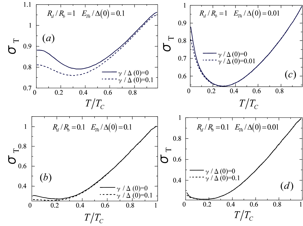
Figure 2: Normalized tunneling conductance for $s$-wave superconductor with $Z=3$. (a) $R_{d}/R_{b}=1$ and $E_{Th}/\Delta(0)=0.1$. (b) $R_{d}/R_{b}=0.1$ and $E_{Th}/\Delta(0)=0.1$. (c) $R_{d}/R_{b}=1$ and $E_{Th}/\Delta(0)=0.01$. (d) $R_{d}/R_{b}=0.1$ and $E_{Th}/\Delta(0)=0.01$.

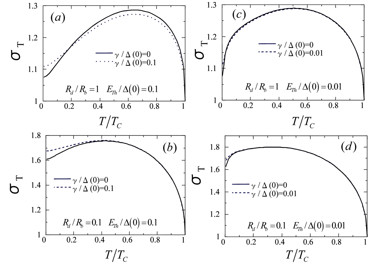
Figure 3: Normalized tunneling conductance for $s$-wave superconductor with $Z=0$. (a) $R_{d}/R_{b}=1$ and $E_{Th}/\Delta(0)=0.1$. (b) $R_{d}/R_{b}=0.1$ and $E_{Th}/\Delta(0)=0.1$. (c) $R_{d}/R_{b}=1$ and $E_{Th}/\Delta(0)=0.01$. (d) $R_{d}/R_{b}=0.1$ and $E_{Th}/\Delta(0)=0.01$.

Next we study the thermal conductance, $\kappa_{T}$, as a function of temperature, where $\kappa_{T}$ is normalized by its value in the normal state, and we fix $E_{Th}/\Delta(0)=0.1$ and $\gamma/\Delta(0)=0$. We will show that $\kappa_{T}$ is almost independent of $E_{Th}/\Delta(0)$ and $\gamma/\Delta(0)$, which implies that the coherent transmission due to the proximity effect does not affect the thermal conductance. Both a quasiparicle just on the Fermi energy and that with finite excitation energy ($\epsilon$) can carry the electric current. The results in Figs. 2 and  3 show the sensitivity of electrical conductance around the zero temperature to $E_{Th}/\Delta(0)$ and $\gamma/\Delta(0)$ because the contribution of a quasiparticle just on the Fermi erengy is governed by the proximity effect. In the case of thermal conductance, on the other hand, only quasiparticles with finite energy can carry heat. At low temperatures, quasiparticles with $\epsilon\sim T\ll T_{c}$ can contribute to $\kappa_{T}$. Such quasiparticles, however, are not allowed in the presence of the gap in superconductors. As a result, $\kappa_{T}$ becomes almost zero around the zero temperature. In high temperatures such as $T\sim T_{C}$, only a quasiparticle with $\epsilon\sim T_{c}$ contributes to $\kappa_{T}$. In such energy range, the quasiparticle spectrum in DN is almost independent of $E_{Th}$ and $\gamma$. Therefore $\kappa_{T}$ is insensitive to $E_{Th}$ and $\gamma$. To substantiate it, we show some numerical examples in Fig. 4 where the independence is confirmed. As shown in Fig. 5, $\kappa_{T}$ increases with increasing $T/T_{C}$ for both $Z=3$ and $Z=0$. Contrary to the case of $\sigma_{T}$, the magnitude of $\kappa_{T}$ is reduced (enhanced) with the increase of $R_{d}/R_{b}$ for $Z=3$ ($Z=0$).

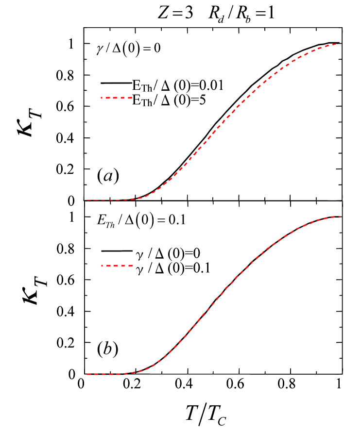
Figure 4: (Color online) Normalized thermal conductance for $s$-wave superconductor with $Z=3$ and $R_{d}/R_{b}=1$. (a) $\gamma/\Delta(0)=0$ and (b) $E_{Th}/\Delta(0)=0.1$.

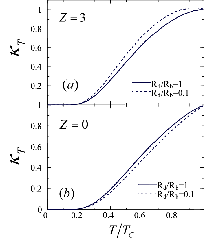
Figure 5: Normalized thermal conductance for $s$-wave superconductor with $E_{Th}/\Delta(0)=0.1$ and $\gamma/\Delta(0)=0$. (a) $Z=3$ and (b) $Z=0$.

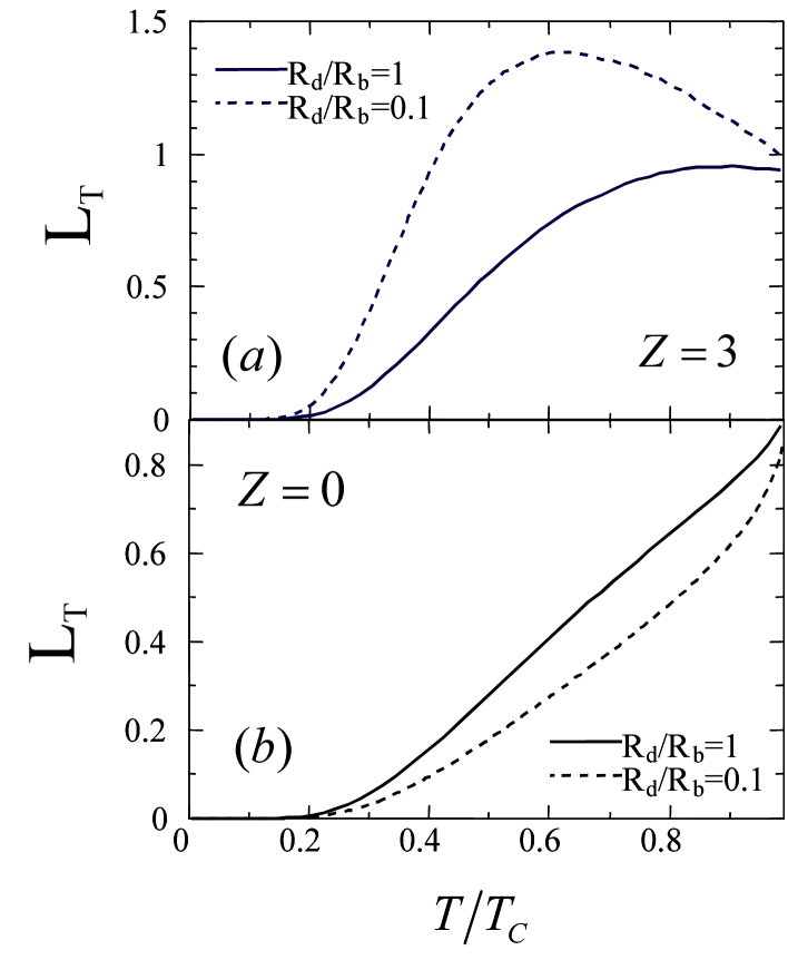
Figure 6: Normalized Lorentz ratio for $s$-wave superconductor with $E_{Th}/\Delta(0)=0.1$ and $\gamma/\Delta(0)=0$. (a) $Z=3$ and (b) $Z=0$.

We plot the Lorentz ratio, $L_{T}$, in Fig. 6 for several $R_{d}/R_{b}$, where $E_{Th}/\Delta(0)=0.1$ and $\gamma/\Delta(0)=0$. We confirmed that the Lorentz ratio is almost independent of $E_{Th}/\Delta(0)$ and $\gamma/\Delta(0)$. The Lorentz ratio is zero for small $T/T_{C}$ and is linear in $T/T_{C}$ in the intermediate region. For $Z=3$ and $R_{d}/R_{b}=0.1$, $L_{T}$ has a peak at $T/T_{C}\sim 0.7$, whereas it is a monotonic increasing function of $T/T_{C}$ for $Z=3$ and $R_{d}/R_{b}=1$ (Fig. 6(a)). For $Z=0$ and $R_{d}/R_{b}=1$, $L_{T}$ is linear in $T/T_{C}$ for $T/T_{C}\geq 0.3$, while for $Z=0$ and $R_{d}/R_{b}=0.1$ , $L_{T}$ is linear in $T/T_{c}$ in the intermediate region (Fig. 6(b)).

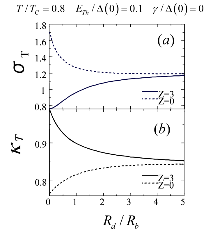
Figure 7: Normalized tunneling conductance (a) and thermal conductance (b) for $s$-wave superconductor with $T/T_{C}=0.8$, $E_{Th}/\Delta(0)=0.1$ and $\gamma/\Delta(0)=0$.

Figure 7 shows $R_{d}/R_{b}$ dependence of tunneling conductance and thermal conductance normalized by their normal values at $T/T_{C}=0.8$, where $E_{Th}/\Delta(0)=0.1$ and $\gamma/\Delta(0)=0$. In low transparent interface (i.e., $Z=3$), the probability of AR increases with increasing $R_{d}/R_{b}$Asano . Thus the magnitude of $\sigma_{T}$ increases with increasing $R_{d}/R_{b}$. On the other hand, $\kappa_{T}$ is a decreasing function of $R_{d}/R_{b}$. In high transparent interface (i.e., $Z=0$), the proximity effect suppresses the electrical conductance because the DN plays a role of the insulating barrier. In this case the probability of AR decreases with increasing $R_{d}/R_{b}$. Thus $\sigma_{T}$ is a decreasing function of $R_{d}/R_{b}$. The results also show that $\kappa_{T}$ is an increasing function of $R_{d}/R_{b}$. In both (a) and (b), $\sigma_{T}$ and $\kappa_{T}$ are close to constants independent of $Z$ for sufficiently large $R_{d}/R_{b}$.

III.2 $d$-wave case

In this subsection, we fix $E_{Th}/\Delta(0)=0.1$ and $\gamma=0$ because $\kappa_{T}$ and $L_{T}$ are insensitive to these parameters. The pair potentials $\Delta_{\pm}(T)$ are given by $\Delta_{\pm}(T)=\Delta(T)\cos[2(\phi\mp\alpha)]$, where $\alpha$ denotes an angle between the normal to the interface and the crystal axis of $d$-wave superconductors, and $\phi$ denotes an injection angle of a quasiparticle measured from the $x$-axis. The amplitude of pair potentials, $\Delta(T)$, is the same as that of $s$-wave superconductors. We choose $0\leq\alpha\leq\pi/4$. It is known that quasiparticles with $\pi/4-\alpha<\phi<\pi/4+\alpha$ can contribute to the MARS at the interface and are responsible for ZBCP in low transparent junctions. It was shown that the proximity effect and MARS do not coexist in the $d$-wave symmetry. In fact, at $\alpha=0$, the MARS does not exist while the proximity effect is possible. On the other hand at $\alpha/\pi=0.25$, the proximity effect is not possible, whereas the MARS appears (see Fig. 1 and Ref. TNGK ). Thus we can expect similar results to the $s$-wave symmetry in the case of $\alpha=0$.

In Fig. 8, we plot the tunneling conductance as a function of temperatures for several choices of $\alpha$, where $R_{d}/R_{b}=0.1$. At $Z=3$ in (a), $\sigma_{T}$ for $\alpha/\pi=0.25$ and 0.125 increase drastically with decreasing temperatures because of the resonant transmission through the MARS. Thus such behavior is not found in $\sigma_{T}$ with $\alpha=0$. In high temperatures, $\sigma_{T}$ for $\alpha/\pi=0$, 0.125 and 0.25 get close together. At $Z=0$, $\sigma_{T}$ is a monotonic decreasing function of $T/T_{C}$ for all $\alpha$. The results show that $\sigma_{T}$ slightly increases with $\alpha$ as shown in (b). The dependence on $\alpha$ of $\sigma_{T}$ at $Z=0$ is very small in comparison with that at $Z=3$.

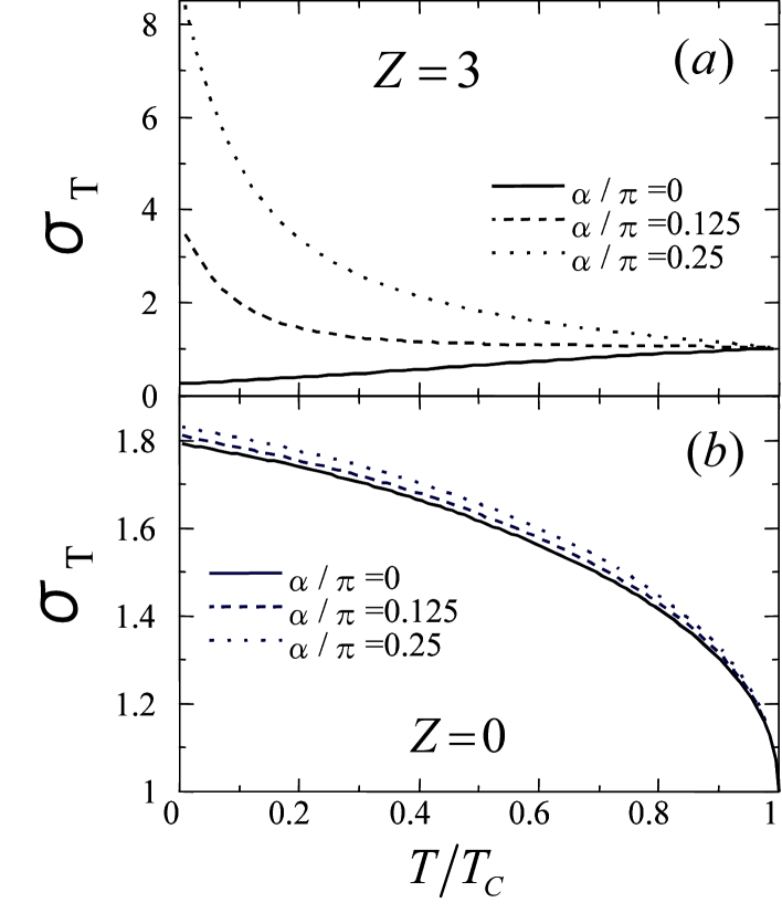
Figure 8: Normalized tunneling conductance for $d$-wave superconductor with $R_{d}/R_{b}=0.1$, $E_{Th}/\Delta(0)=0.1$ and $\gamma/\Delta(0)=0$. (a) $Z=3$ and (b) $Z=0$.

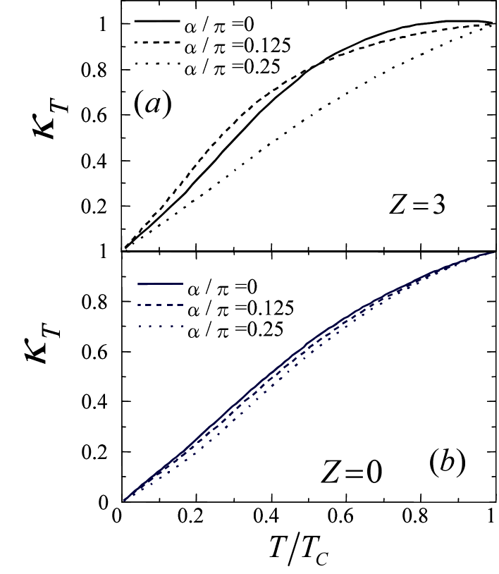
Figure 9: Normalized thermal conductance for $d$-wave superconductor with $R_{d}/R_{b}=0.1$, $E_{Th}/\Delta(0)=0.1$ and $\gamma/\Delta(0)=0$. (a) $Z=3$ and (b) $Z=0$.

In Fig. 9, we show thermal conductance as a function of temperatures for several $\alpha$ with $R_{d}/R_{b}=0.1$. In both $Z=3$ and 0, $\kappa_{T}$ are monotonic increasing function of $T/T_{C}$ and are proportional to $T/T_{C}$ for small $T/T_{C}$. This linear dependence of $\kappa_{T}$ for low temperatures is not seen in the $s$-wave symmetry (Fig. 5) and reflects the line nodes of the pair potential. The results also show that $\kappa_{T}$ depends on $\alpha$ for $Z=3$ in (a), whereas it is almost independent of $\alpha$ for $Z=0$ in (b).

In Fig. 10, the Lorentz ratio is shown for several $\alpha$, where $R_{d}/R_{b}=0.1$. The Lorentz ratio has a peak at $T/T_{C}\sim 0.4$ for $Z=3$ and $\alpha=0$ as shown in (a). This peak gradually disappears with increasing $\alpha$. For $Z=0$, $L_{T}$ is proportional to $T/T_{C}$ almost independent of $\alpha$ as shown in (b).

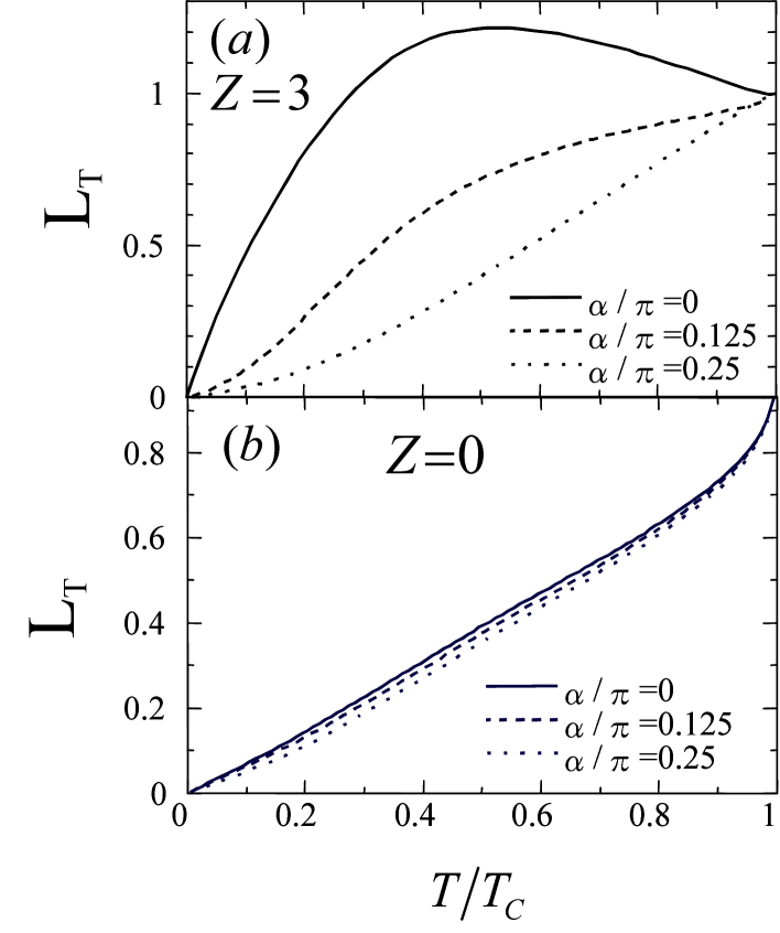
Figure 10: Normalized Lorenz ratio for $d$-wave superconductor with $R_{d}/R_{b}=0.1$, $E_{Th}/\Delta(0)=0.1$ and $\gamma/\Delta(0)=0$. (a) $Z=3$ and (b) $Z=0$.

Figures 11 and 12 show $R_{d}/R_{b}$ dependence of tunneling conductance and thermal conductance which are normalized by their normal values at $T/T_{C}=0.8$. For $Z=3$ $\sigma_{T}$ is an increasing function of $R_{d}/R_{b}$ for $\alpha/\pi=0$ as shown in Fig. 11 (a) because the probability of the AR increases with increasing $R_{d}/R_{b}$ as in the $s$-wave symmetry. The peaks at $R_{d}/R_{b}=0$ in $\alpha/\pi=0.25$ and 0.125 is a consequence of the MARS. The impurity scatterings in DN simply suppress the magnitude of $\sigma_{T}$ at $\alpha/\pi=0.25$ because the the proximity effect is absent in this case. As a result, $\sigma_{T}$ becomes a decreasing function of $R_{d}/R_{b}$ at $\alpha/\pi=0.25$ as shown in Fig. 11 (a). For sufficiently large $R_{d}/R_{b}$, $\sigma_{T}$ is close to a constant. For $\alpha/\pi=0$ $\kappa_{T}$ is a decreasing function of $R_{d}/R_{b}$ while it is an increasing function of $R_{d}/R_{b}$ for $\alpha/\pi=0.125$ and $\alpha/\pi=0.25$ as shown in Fig. 11 (b). For sufficiently large $R_{d}/R_{b}$, $\kappa_{T}$ is close to a constant for all $\alpha$. In Fig. 11(b), we find that the formation of the MARS suppresses $\kappa_{T}$. This can be interpreted as follows. When the MARS is formed at the interface, the quasiparticle density of states becomes large around the zero energy. Such states around the zero energy, however, can not carry the heat. The zero energy peak in the density of states means suppression of the density of states in higher energies which can carry the heat. Thus the formation of the MARS suppresses the thermal conductance. At $Z=0$ in Fig. 12, the probability of the AR decreases as increasing $R_{d}/R_{b}$ for all $\alpha$. The line shapes of $\sigma_{T}$ and $\kappa_{T}$ are understood in the same way as those in the $s$-wave case with $Z=0$ in Fig. 7.

Figure 11: Normalized tunneling conductance (a) and thermal conductance (b) for $d$-wave superconductor with $T/T_{C}=0.8$, $Z=3$, $E_{Th}/\Delta(0)=0.1$ and $\gamma/\Delta(0)=0$.

Figure 12: Normalized tunneling conductance (a) and thermal conductance (b) for $d$-wave superconductor with $T/T_{C}=0.8$, $Z=0$, $E_{Th}/\Delta(0)=0.1$ and $\gamma/\Delta(0)=0$.

III.3 $p$-wave case

Here we also fix $E_{Th}/\Delta(0)=0.1$ and $\gamma=0$ because $\kappa_{T}$ and $L_{T}$ are insensitive to these parameters. We choose the pair potentials $\Delta_{\pm}$ as $\Delta_{\pm}=\pm\Delta(T)\cos[(\phi\mp\alpha)]$ where $\alpha$ denotes an angle between the normal to the interface and the lobe direction of the $p$-wave pair potential and $\Delta(T)$ is the maximum amplitude of the pair potential. In the following, we choose $0\leq\alpha\leq\pi/2$. It is known that quasiparticles with injection angle $\phi$ with $-\pi/2+\alpha<\phi<\pi/2-\alpha$ can contribute to the formation of the MARS at the interface. In particular at $\alpha=0$, the MARS and the proximity effect perfectly coexist, which causes the penetration of the resonant states into the DN p-wave . On the other hand, for $\alpha/\pi=0.5$, neither the MARS nor the proximity effect exist (see Fig. 1 and Ref. p-wave, ).

In Fig. 13, we show the calculated results of tunneling conductance for several $\alpha$, where $R_{d}/R_{b}=0.1$. At $Z=3$, $\sigma_{T}$ for $\alpha/\pi=0$ and 0.25 increases drastically with the decrease of temperatures because of the resonant transmission via the MARS, while the result for $\alpha/\pi=0.5$ monotonically increases with $T$. In the case of $Z=0$, $\sigma_{T}$ increases with decreasing $T$ irrespective of $\alpha$.

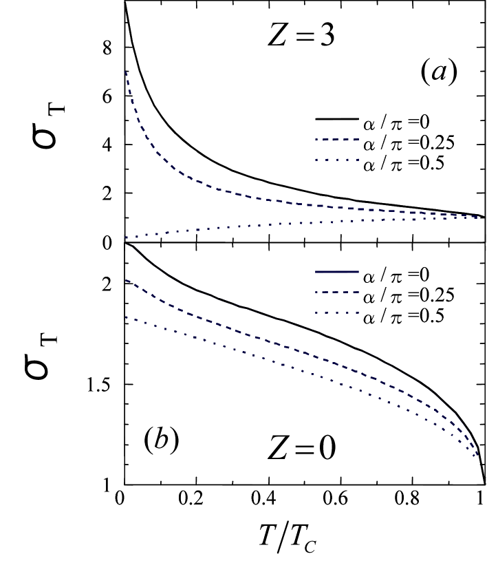
Figure 13: Normalized tunneling conductance for $p$-wave superconductor with $R_{d}/R_{b}=0.1$, $E_{Th}/\Delta(0)=0.1$ and $\gamma/\Delta(0)=0$. (a) $Z=3$ and (b) $Z=0$.

The thermal conductance in Fig. 14 is a monotonic increasing function of $T/T_{C}$, where $R_{d}/R_{b}=0.1$. Except for $\alpha=0$, $\kappa_{T}$ is proportional to $T$ for small $T/T_{C}$. This behavior is also found in the $d$-wave symmetry in Fig. 9 and stems from the line nodes in the pair potentials. At $\alpha=0$, $\kappa_{T}$ is expected to be an exponential function of $T/T_{C}$. Thus $\kappa_{T}$ increases with increasing $\alpha$ as shown in both $Z=3$ and 0. Although line node of the pair potential exists in this case, $\kappa_{T}$ has an exponential dependence on $T$ as in the $s$-wave case because the direction of the line node is perpendicular to that of the thermal current.

Figure 14: Normalized thermal conductance for $p$-wave superconductor with $R_{d}/R_{b}=0.1$, $E_{Th}/\Delta(0)=0.1$ and $\gamma/\Delta(0)=0$. (a) $Z=3$ and (b) $Z=0$.

The Lorentz ratio has a peak at $T/T_{C}\sim 0.3$ for $\alpha=0$ and $Z=3$, as shown in Fig. 15(a). This peak tends to disappear for larger $\alpha$. At $Z=0$ $L_{T}$ linearly increases with the increase of temperatures in intermediate temperature regime as shown in (b).

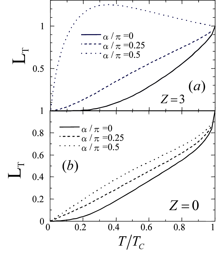
Figure 15: Normalized Lorenz ratio for $p$-wave superconductor with $R_{d}/R_{b}=0.1$, $E_{Th}/\Delta(0)=0.1$ and $\gamma/\Delta(0)=0$. (a) $Z=3$ and (b) $Z=0$.

Figures 16 and 17 display $R_{d}/R_{b}$ dependence of tunneling conductance and thermal conductance at $T/T_{C}=0.8$. The results are normalized by their normal values at $T/T_{C}=0.8$. At $Z=3$, $\sigma_{T}$ has a reentrant behavior in $R_{d}/R_{b}$ for small $\alpha$ as shown in Fig. 16 (a). It is noted that the finite energy states and the zero energy states contribute to the conductance in qualitatively different ways. In finite energies, $\sigma_{T}$ decreases with increasing $R_{d}/R_{b}$ because the probability of the AR decreases with increasing $R_{d}/R_{b}$. On the other hand at the zero energy, $\sigma_{T}$ increase with the increase of $R_{d}/R_{b}$ due to the formation of the resonant statesp-wave . For small (large) $R_{d}/R_{b}$, the contribution of the finite energies states (the zero energy states) dominates $\sigma_{T}$. This explains the reentrant behavior in $\sigma_{T}$. In contrast to $\alpha=0$, $\sigma_{T}$ for $\alpha=0.5\pi$ is almost constant as shown in Fig. 16 (a) because there are neither the proximity effect nor the MARS. The characteristics of the thermal conductance can be understood in a similar way. We note that the zero energy states never contribute to the thermal transport. At $\alpha=0$, $\kappa_{T}$ increases with increasing of $R_{d}/R_{b}$ in contrast to the $d$-wave case with $\alpha=0$. This difference stems from the existence of the MARS. At $\alpha/\pi=0.5$, $\kappa_{T}$ is almost constant as shown in Fig. 16 (b). The line shapes of $\sigma_{T}$ and $\kappa_{T}$ for $\alpha=0$ and $0.25\pi$ at $Z=0$ in Fig. 17 are qualitatively similar to those for $Z=3$. For $\alpha/\pi=0.5$, $\sigma_{T}$ decreases with $R_{d}/R_{b}$ and $\kappa_{T}$ increases with $R_{d}/R_{b}$. These behaviors can be explained by the fact that the probability of the AR decreases as increasing $R_{d}/R_{b}$. From Fig. 16(b) for small $R_{d}/R_{b}$, we can also find that the MARS suppresses $\kappa_{T}$.

Figure 16: Normalized tunneling conductance (a) and thermal conductance (b) for $p$-wave superconductor with $T/T_{C}=0.8$, $Z=3$, $E_{Th}/\Delta(0)=0.1$ and $\gamma/\Delta(0)=0$.

Figure 17: Normalized tunneling conductance (a) and thermal conductance (b) for $p$-wave superconductor with $T/T_{C}=0.8$, $Z=0$, $E_{Th}/\Delta(0)=0.1$ and $\gamma/\Delta(0)=0$.

On the basis of calculated results of electrical and thermal conductance, we propose a way to classify the pairing symmetries with several orientation angles into six groups as shown in Fig. 18. We have studied seven junctions: $s$-wave superconductor (s), $d$-wave superconductor with $\alpha=0$ (d($\alpha=0$)), $d$-wave superconductor with $\alpha/\pi=0.125$ (d($\alpha/\pi=0.125$)), $d$-wave superconductor with $\alpha/\pi=0.25$ (d($\alpha/\pi=0.25$)), $p$-wave superconductor with $\alpha=0$ (p($\alpha=0$)), $p$-wave superconductor with $\alpha/\pi=0.25$ (p($\alpha/\pi=0.25$)) and $p$-wave superconductor with $\alpha/\pi=0.5$ (p($\alpha/\pi=0.5$)). We focus on the results with $Z=3$ because symmetries of pair potentials are better characterized by transport properties in lower transparent junctions. Checking the line shapes of $\sigma_{T}$ and $\kappa_{T}$, we can separate these junctions into four groups as shown in the first and the second processes of Fig. 18(see Figs. 2, 5, 8, 9, 13, 14 and TABLE I). Next applying a weak magnetic field $H$ parallel to the junction plane, $\sigma_{T}$ for d($\alpha=0$) and p($\alpha/\pi=0.25$) junctions decreases as increasing magnetic field as shown in Fig. 19 since the proximity effect is suppressed by the applied magnetic field Belzig1 . On the other hand $\sigma_{T}$ for d($\alpha/\pi=0.125$), d($\alpha/\pi=0.25$) or p($\alpha/\pi=0.5$) junctions is robust against applied magnetic field since there is almost no proximity effect (third process in Fig. 18). We note that the pair-breaking rate $\gamma$ is given by $e^{2}w^{2}DH^{2}/6$, where $w$ is the transverse size of the DNBelzig1 . Assuming $w=10^{-5}m$, $D=10^{-3}m^{2}/s$, $\Delta(0)=10^{-3}eV$, and $H=10^{-2}T$, we can estimate the pair-breaking rate $\gamma/\Delta(0)\sim 1$. Distinguishing p($\alpha/\pi=0.25$) from d($\alpha/\pi=0.125$) is a delicate problem since both of them have the proximity effect and the MARS. The two junctions, however, have qualitative difference in the density of states (DOS) in DN. In p($\alpha/\pi=0.25$) junctions, the DOS has a zero energy peak due to the formation of the resonant states whereas the DOS in the d($\alpha/\pi=0.125$) junctions does not show such zero energy peak p-wave . As a result, the conductance measurable by scanning tunneling spectroscopy (STS), $\sigma_{0}$, reflects these features. Here $\sigma_{0}$ is defined as

$$\sigma_{0}=\frac{1}{2T}\int_{0}^{\infty}\frac{\text{Re}\cos\theta d\epsilon}{\cosh^{2}[\frac{\epsilon}{2T}]}$$ (29)

and $\text{Re}\cos\theta$ is the DOS normalized by its normal states value. We plot it at $x=3L/4$ as a function of $T/T_{C}$ in Fig. 20. In p($\alpha/\pi=0.25$) junctions, a peak appears at zero temperature in contrast to the case of the d($\alpha/\pi=0.125$) junctions. Thus we can easily distinguish these superconductors by STS.

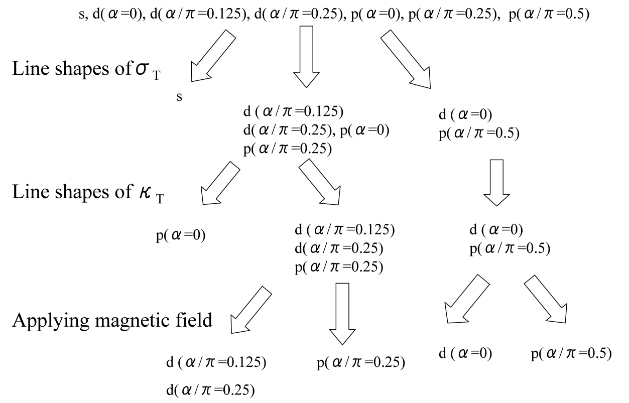
Figure 18: Chart for distinguishing $s$-, $d$- and $p$-wave superconductors.

Figure 19: Magnetic field dependence of normalized tunneling conductance with $Z=3$ and $E_{Th}/\Delta(0)=0.1$ for (a) $d$-wave superconductor with $\alpha/\pi=0$ and (b) $p$-wave superconductor with $\alpha/\pi=0.25$.

Figure 20: The conductance measurable by STS at $x=3L/4$ with $Z=3$, $R_{d}/R_{b}=0.1$, $E_{Th}/\Delta(0)=0.1$ and $\gamma/\Delta(0)=0$ for $d$-wave superconductor with $\alpha/\pi=0.125$ and for $p$-wave superconductor with $\alpha/\pi=0.25$.

Table 1: Low temperature dependences of $\sigma_{T}$ and $\kappa_{T}$.

pairing symmetry	$\sigma_{T}$	$\kappa_{T}$
s	reentrant	exponential
d($\alpha=0$)	linear	linear
d($\alpha/\pi=0.125$)	inverse	linear
d($\alpha/\pi=0.25$)	inverse	linear
p($\alpha=0$)	inverse	exponential
p($\alpha/\pi=0.25$)	inverse	linear
p($\alpha/\pi=0.5$)	linear	linear

IV Conclusions

In the present paper, we have derived a general expression of the thermal conductance in normal metal / superconductor junctions based on the Usadel equation under the generalized boundary condition. We have studied the electrical and thermal transport in diffusive normal metal / $s$-, $d$- and $p$-wave superconductor junctions in the presence of magnetic impurities in normal metals. The main conclusions are summarized as follows.

1. The proximity effect does not influence the thermal conductance. This statement is illustrated with some numerically calculated examples.

2. The midgap Andreev resonant states in $d$- or $p$-wave superconductor junctions suppress the thermal conductance. The formation of MARS drastically gathers the density of states at the Fermi energy near the DN/S interface. Such quasiparticles, however, do not carry heat because excitation energies of them are almost zero.

3. The thermal conductance of the junctions reflects the existence of the line nodes of the pair potential except for the case that the direction of the line node is perpendicular to that of the thermal current.

Electric conductance, thermal conductance, and their Lorentz ratio calculated as a function of temperature depend strongly on a pairing symmetry of a superconductor. This fact indicates a possibility of distinguishing one pairing symmetry from another by careful comparison of the present calculations and experimental results.

In this paper, we have focused on N/S junctions of unconventional superconductors. So far an extension of the circuit theory to long diffusive S/N/S junctions has been performed by Bezuglyi et al. Bezuglyi2 in $s$-wave symmetry. In S/N/S junctions, the multiple AR produces subharmonic gap structures in I-V curves M1 ; M2 ; M3 ; M4 ; M5 ; M6 ; M7 ; M8 . In S/N/S junctions of unconventional superconductors, it is known that MARS leads to the anomalous current-phase relation and temperature dependence of the Josephson current TKJ . Effects of unconventional superconductivity of such I-V curves are an important future issue. The research in this direction is now in progress and the results will be reported elsewhere.

The authors appreciate useful and fruitful discussions with J. Inoue, Yu. Nazarov and H. Itoh. This work was supported by NAREGI Nanoscience Project, the Ministry of Education, Culture, Sports, Science and Technology, Japan, the Core Research for Evolutional Science and Technology (CREST) of the Japan Science and Technology Corporation (JST) and a Grant-in-Aid for the 21st Century COE ”Frontiers of Computational Science” . The computational aspect of this work has been performed at the Research Center for Computational Science, Okazaki National Research Institutes and the facilities of the Supercomputer Center, Institute for Solid State Physics, University of Tokyo and the Computer Center.

V Appendix

Here we calculate the matrix current for the calculation of the thermal conductance of $d$-wave junctions. We denote $\check{H}_{+}$, $\check{H}_{-}$, $\check{B}_{n}$, $\check{I}$ as follows,

$$\check{H}_{+}=\left(\begin{array}[]{cc}\hat{R}_{p}&\hat{K}_{p}\\ 0&\hat{A}_{p}\end{array}\right),\ \ \check{H}_{-}=\left(\begin{array}[]{cc}\hat{R}_{m}&\hat{K}_{m}\\ 0&\hat{A}_{m}\end{array}\right),$$ (34)

$$\check{B}_{n}=\left(\begin{array}[]{cc}\hat{B}_{R}&\hat{B}_{K}\\ 0&\hat{B}_{A}\end{array}\right),\ \ \check{I}=\left(\begin{array}[]{cc}\hat{I}_{R}&\hat{I}_{K}\\ 0&\hat{I}_{A}\end{array}\right)$$

with $\check{H}_{\pm}=(\check{G}_{2+}\pm\check{G}_{2-})/2.$ In singlet superconductors, we can choose $\hat{R}_{1}=\cos\theta(x)\hat{\tau}_{3}+\sin\theta(x)\hat{\tau}_{2}$ to satisfy the boundary condition at the interface.

The matrix current is given by $\check{I}=\mathrm{Tr}_{n}[\check{I_{n}}]$ with $\check{I_{n}}=2[\check{G}_{1},\check{B}_{n}]$ and

$$\check{B}_{n}=(-T_{1n}[\check{G}_{1},\check{H}_{-}^{-1}]+\check{H}_{-}^{-1}\check{H}_{+}-T_{1n}^{2}\check{G}_{1}\check{H}_{-}^{-1}\check{H}_{+}\check{G}_{1})^{-1}(T_{1n}(1-\check{H}_{-}^{-1})+T_{1n}^{2}\check{G}_{1}\check{H}_{-}^{-1}\check{H}_{+})$$ (35)

where

$$T_{1n}=\frac{T_{n}}{2-T_{n}+2\sqrt{1-T_{n}}}.$$

Next, we focus on the Keldysh component. We define $I_{b}$

$$I_{b}=\frac{1}{2}\sum_{n}\mathrm{Tr}[\hat{I}_{K}].$$ (36)

After straightforward calculations, $I_{b}$ is given by

$$I_{b}=\frac{1}{2}\sum_{n}\mathrm{Tr}[(\hat{R}_{1}-\hat{A}_{1})\hat{B}_{K}+f_{l}(L_{-})(\hat{R}_{1}-\hat{A}_{1})(\hat{B}_{A}-\hat{B}_{R})].$$

It is necessary to obtain $\hat{B}_{K}$ which is given by

$$\hat{B}_{K}=\hat{D}_{R}^{-1}\hat{N}_{K}-\hat{D}_{R}^{-1}\hat{D}_{K}\hat{D}_{A}^{-1}\hat{N}_{A},$$ (37)

with

$$\check{D}=-T_{1n}[\check{G}_{1},\check{H}_{-}^{-1}]+\check{H}_{-}^{-1}\check{H}_{+}-T_{1n}^{2}\check{G}_{1}\check{H}_{-}^{-1}\check{H}_{+}\check{G}_{1},\ \ \check{D}=\left(\begin{array}[]{cc}\hat{D}_{R}&\hat{D}_{K}\\ 0&\hat{D}_{A}\end{array}\right),$$

where $\hat{N}_{K}$ and $\hat{N}_{A}$ is the Keldysh and advanced part of $\check{N}$ given by

$$\check{N}=T_{1n}-T_{1n}\check{H}_{-}^{-1}+T_{1n}^{2}\check{G}_{1}\check{H}_{-}^{-1}\check{H}_{+}\ \ \check{N}=\left(\begin{array}[]{cc}\hat{N}_{R}&\hat{N}_{K}\\ 0&\hat{N}_{A}\end{array}\right).$$

We can express $\hat{N}_{K}$ and $\hat{D}_{K}$ as linear combination of distribution functions $f_{S}$, $f_{l}(L_{-})$, and $f_{t}(L_{-})$ as follows,

$$\hat{N}_{K}=\hat{C}_{1}f_{S}+\hat{C}_{2}f_{l}(L_{-})+\hat{C}_{3}f_{t}(L_{-}),$$

$$\hat{D}_{K}=\hat{C}_{4}f_{S}+\hat{C}_{5}f_{l}(L_{-})+\hat{C}_{6}f_{t}(L_{-}),$$

by $2\times 2$ matrix $C_{i}$ $(i=1-6)$. Taking account of the fact that $\hat{D}_{R}^{-1}\hat{C}_{1}$, $\hat{D}_{R}^{-1}\hat{C}_{2}$, $\hat{D}_{R}^{-1}\hat{C}_{4}\hat{D}_{A}^{-1}\hat{N}_{A}$ and $\hat{D}_{R}^{-1}\hat{C}_{5}\hat{D}_{A}^{-1}\hat{N}_{A}$ can be expressed by the linear combination of $\hat{\tau}_{2}$ and $\hat{\tau}_{3}$, while $\hat{D}_{R}^{-1}\hat{C}_{3}$ and $\hat{D}_{R}^{-1}\hat{C}_{6}\hat{D}_{A}^{-1}\hat{N}_{A}$ are proportional to the linear combination of $\hat{1}$ and $\hat{\tau}_{1}$, we can express $I_{b}$ as follows,

$$I_{b}=\frac{1}{2}\sum_{n}\mathrm{Tr}[f_{S}{(\hat{R}_{1}-\hat{A}_{1})(\hat{D}_{R}^{-1}\hat{C}_{1}-\hat{D}_{R}^{-1}\hat{C}_{4}\hat{D}_{A}^{-1}\hat{N}_{A})}+f_{l}(L_{-}){(\hat{R}_{1}-\hat{A}_{1})(\hat{D}_{R}^{-1}\hat{C}_{2}-\hat{D}_{R}^{-1}\hat{C}_{5}\hat{D}_{A}^{-1}\hat{N}_{A})+(\hat{R}_{1}-\hat{A}_{1})(\hat{B}_{A}-\hat{B}_{R})}]$$

with

$$\hat{C}_{1}=T_{1n}[\hat{A}_{m}^{-1}-\hat{R}_{m}^{-1}+T_{1n}(\hat{R}_{1}\hat{R}_{m}^{-1}(\hat{R}_{p}-\hat{A}_{p})-\hat{R}_{1}(\hat{A}_{m}^{-1}-\hat{R}_{m}^{-1})\hat{A}_{p})]$$

$$\hat{C}_{2}=T_{1n}^{2}(\hat{R}_{1}-\hat{A}_{1})\hat{A}_{m}^{-1}\hat{A}_{p}$$

$$\hat{C}_{4}=T_{1n}[\hat{R}_{1}(\hat{A}_{m}^{-1}-\hat{R}_{m}^{-1})-(\hat{A}_{m}^{-1}-\hat{R}_{m}^{-1})\hat{A}_{1}]+\hat{R}_{m}^{-1}\hat{R}_{p}-\hat{A}_{m}^{-1}\hat{A}_{p}+T_{1n}^{2}[-\hat{R}_{1}\hat{R}_{m}^{-1}(\hat{R}_{p}-\hat{A}_{p})\hat{A}_{1}+\hat{R}_{1}(\hat{A}_{m}^{-1}-\hat{R}_{m}^{-1})\hat{A}_{p}\hat{A}_{1}]$$

$$\hat{C}_{5}=T_{1n}[-(\hat{R}_{1}-\hat{A}_{1})\hat{A}_{m}^{-1}+\hat{R}_{m}^{-1}(\hat{R}_{1}-\hat{A}_{1})-T_{1n}(\hat{R}_{1}\hat{R}_{m}^{-1}\hat{R}_{p}(\hat{R}_{1}-\hat{A}_{1})+(\hat{R}_{1}-\hat{A}_{1})\hat{A}_{m}\hat{A}_{p}^{-1}\hat{A}_{1})].$$ (38)

We use the following equations

$$\hat{D}_{R}^{-1}(T_{1n}-T_{1n}\hat{R}_{m}^{-1}+T_{1n}^{2}\hat{R}_{1}\hat{R}_{m}^{-1}\hat{R}_{p})=\hat{B}_{R},$$

$$\hat{B}_{R}(1+\hat{R}_{m}^{-1}+T_{1n}\hat{R}_{1}\hat{R}_{p}\hat{R}_{m}^{-1})=T_{1n}\hat{R}_{m}^{-1}\hat{R}_{p}$$ (39)

where $\hat{B}_{R}$ is given as $\hat{B}_{R}=b_{1}\hat{\tau}_{1}+b_{2}\hat{\tau}_{2}+b_{3}\hat{\tau}_{3}$ with

$$b_{1}=\frac{-iT_{1n}(f_{+}g_{-}-f_{-}g_{+})}{(1+T_{1n}^{2})(1+g_{+}g_{-}+f_{+}f_{-})+2T_{1n}[\cos\theta_{L}(g_{+}+g_{-})+\sin\theta_{L}(f_{+}+f_{-})]},$$

$$b_{2}=\frac{-T_{1n}[T_{1n}\sin\theta_{L}(1+g_{+}g_{-}+f_{+}f_{-})+f_{+}+f_{-}]}{(1+T_{1n}^{2})(1+g_{+}g_{-}+f_{+}f_{-})+2T_{1n}[\cos\theta_{L}(g_{+}+g_{-})+\sin\theta_{L}(f_{+}+f_{-})]},$$

$$b_{3}=\frac{-T_{1n}[T_{1n}\cos\theta_{L}(1+g_{+}g_{-}+f_{+}f_{-})+g_{+}+g_{-}]}{(1+T_{1n}^{2})(1+g_{+}g_{-}+f_{+}f_{-})+2T_{1n}[\cos\theta_{L}(g_{+}+g_{-})+\sin\theta_{L}(f_{+}+f_{-})]}.$$ (40)

Finally we reach the expression of $I_{b}$ given by the following equation.

$$I_{b}=\sum_{n}\frac{T_{n}}{2}\frac{C_{0}^{\prime}(f_{s}-f_{l}(L_{-}))}{\mid(2-T_{n})(1+g_{+}g_{-}+f_{+}f_{-})+T_{n}[\cos\theta_{L}(g_{+}+g_{-})+\sin\theta_{L}(f_{+}+f_{-})]\mid^{2}}$$ (41)

$$C_{0}^{\prime}=T_{n}(1+\mid\cos\theta_{L}\mid^{2}-\mid\sin\theta_{L}\mid^{2})(\mid g_{+}+g_{-}\mid^{2}-\mid f_{+}+f_{-}\mid^{2}+\mid 1+f_{+}f_{-}+g_{+}g_{-}\mid^{2}-\mid f_{+}g_{-}-g_{+}f_{-}\mid^{2})$$

$$+4(2-T_{n})[\mathrm{Real}[{(1+g_{+}^{\ast}g_{-}^{\ast}+f_{+}^{\ast}f_{-}^{\ast})(g_{+}+g_{-})}]\mathrm{Real}(\cos\theta_{L})-\mathrm{Imag}(\sin\theta_{L})\mathrm{Imag}[{(1+g_{+}^{\ast}g_{-}^{\ast}+f_{+}^{\ast}f_{-}^{\ast})(f_{+}+f_{-})}]]$$

$$+4T_{n}\mathrm{Real}(\cos\theta_{L}\sin\theta_{L}^{\ast})\mathrm{Real}[(f_{+}+f_{-})(g_{+}^{\ast}+g_{-}^{\ast})].$$

This is a general expression applicable to any singlet superconductors without broken time reversal symmetry state.

References

(1) G. Wiedemann and R. Franz, Ann. Phys. 89, 497 (1853).
(2) M. J. Kearney and P. N. Butcher, J. Phys. C. Solid State
Phys. 21, L265 (1988).
(3) C. Castellani, C. DiCastro, G. Kotliar, P. A Lee and G.
Strinati, Phys. Rev. Lett. 59, 477 (1987).
(4) G. V. Chester, A. Tellung, Proc. Phys. Soc. 77,
1005 (1961).
(5) L. Smrcka, and P. Streda, J. Phys. C. Solid State Phys.
10, 2153 (1977).
(6) N. P. Ong, Phys. Rev. B 43, 193 (1991).
(7) R. W. Hill, C. Proust, L. Taillefer, P. Founier, R. L.
Greene, Nature 414, 711 (2001).
(8) J. Bardeen, G. Rickayzen and L. Tewordt, Phys. Rev. 113, 982 (1959).
(10) G.E. Blonder, M. Tinkham, and T.M. Klapwijk, Phys. Rev. B
25, 4515 (1982).
(11) A. Bardas and D. Averin, Phys. Rev. B 52, 12873
(1995).
(12) I. A. Devyatov, M. Y. Kupriyanov, L. S. Kuzmin, A. A.
Golubov and M. Willander, JETP 90, 1050 (2000).
(13) F. W. J. Hekking and Yu. V. Nazarov, Phys. Rev. Lett.
71, 1625 (1993).
(14) F. Giazotto, P. Pingue, F. Beltram, M. Lazzarino, D.
Orani, S. Rubini, and A. Franciosi, Phys. Rev. Lett. 87, 216808
(2001).
(15) T.M. Klapwijk, Physica B 197, 481 (1994).
(16) A. Kastalsky, A.W. Kleinsasser, L.H. Greene, R. Bhat,
F.P. Milliken, J.P. Harbison, Phys. Rev. Lett. 67, 3026 (1991).
(17) C. Nguyen, H. Kroemer and E.L. Hu, Phys. Rev. Lett. 69, 2847 (1992).
(18) B.J. van Wees, P. de Vries, P. Magnee, and T.M. Klapwijk,
Phys. Rev. Lett. 69, 510 (1992).
(19) J. Nitta, T. Akazaki and H. Takayanagi, Phys. Rev. B 49 3659 (1994).
(20) S.J.M. Bakker, E. van der Drift, T.M. Klapwijk, H.M.
Jaeger, and S. Radelaar, Phys. Rev. B 49, 13275 (1994).
(21) P. Xiong, G. Xiao and R.B. Laibowitz, Phys. Rev. Lett.
71, 1907 (1993).
(22) P.H.C. Magnee, N. van der Post, P.H.M. Kooistra, B.J. van
Wees, and T.M. Klapwijk, Phys. Rev. B 50, 4594 (1994).
(23) J. Kutchinsky, R. Taboryski, T. Clausen, C. B. Sorensen, A.
Kristensen, P. E. Lindelof, J. Bindslev Hansen, C. Schelde Jacobsen, and J.
L. Skov, Phys.Rev. Lett. 78 ,931 (1997).
(24) W. Poirier, D. Mailly, and M. Sanquer, Phys. Rev. Lett.
79, 2105 (1997).
(27) A.I. Larkin and Yu. V. Ovchinnikov, Sov. Phys. JETP 41, 960 (1975)
(28) A.F. Volkov, A.V. Zaitsev and T.M. Klapwijk, Physica C
210, 21 (1993).
(29) C. J. Lambert, R. Raimondi, V. Sweeney and A. F. Volkov,
Phys. Rev. B 55, 6015 (1997).
(30) Yu. V. Nazarov, Phys. Rev. Lett. 73, 1420 (1994).
(31) S. Yip, Phys. Rev. B 52, 3087 (1995).
(32) Yu. V. Nazarov and T. H. Stoof, Phys. Rev. Lett. 76, 823 (1996); T. H. Stoof and Yu. V. Nazarov, Phys. Rev. B 53,
14496 (1996).
(33) A. F. Volkov, N. Allsopp, and C. J. Lambert, J. Phys.
Cond. Mat. 8, L45 (1996); A. F. Volkov and H. Takayanagi, Phys.
Rev. B 56, 11184 (1997).
(34) A.A. Golubov, F.K. Wilhelm, and A.D. Zaikin, Phys. Rev. B
55, 1123 (1997).
(35) A.F. Volkov and H. Takayanagi, Phys. Rev. B 56, 11184 (1997).
(36) R. Seviour and A. F. Volkov, Phys. Rev. B 61,
R9273 (2000).
(37) W. Belzig, F. K. Wilhelm, C. Bruder, et al.,
Superlattices and Microstructures 25, 1251 (1999).
(38) S. Yip, Phys. Rev. B 52, 15504 (1995).
(39) T. Yokoyama, Y. Tanaka, A. A. Golubov, J. Inoue, and Y.
Asano, Phys. Rev. B 71, 094506 (2005).
(40) M.Yu. Kupriyanov and V. F. Lukichev, Zh. Exp. Teor. Fiz.
94 (1988) 139 [Sov. Phys. JETP 67, (1988) 1163].
(41) A. V. Zaitsev, Sov. Phys. JETP 59, 1163 (1984).
(42) Yu. V. Nazarov, Superlattices and Microstructuctures
25, 1221 (1999).
(43) Y. Tanaka, A. A. Golubov and S. Kashiwaya, Phys. Rev. B
68 054513 (2003).
(44) R. Raimondi, G. Savona, P. Schwab and T. Lück, Phys.
Rev. B 70, 155109 (2004).
(45) J. Beyer-Nielsen and H. Smith, Phys. Rev. B 31,
2831 (1985).
(46) M. J. Graf, S-K. Yip, J . A. Sauls and D. Rainer Phys. Rev. B
53, 15147 (1996).
(47) M. J. Graf and A. V. Balatsky, Phys. Rev. B 62,
9697 (2000); M. J. Graf, S-K. Yip and J . A. Sauls, Phys. Rev. B 62, 14393 (2000).
(48) E. V. Bezuglyi and V. Vinokur, Phys. Rev. Lett. 91, 137002 (2003).
(49) R. Movshovich, M. A. Hubbard, M. B. Salamon, A. V.
Balatsky, R. Yoshizaki, J. L. Sarrao, and M. Jaime Phys. Rev. Lett. 80, 1968 (1998).
(50) R. Movshovich, M. Jaime, J. D. Thompson, C. Petrovic,
Z. Fisk, P. G. Pagliuso, and J. L. Sarrao Phys. Rev. Lett. 86, 5152
(2001).
(51) M. Chiao, R. W. Hill, C. Lupien, B. Popic, R. Gagnon, and L.
Taillefer Phys. Rev. Lett. 82, 2943 (1999).
(52) K. Izawa, H. Takahashi, H. Yamaguchi, Yuji Matsuda, M.
Suzuki, T. Sasaki, T. Fukase, Y. Yoshida, R. Settai, and Y. Onuki Phys. Rev.
Lett. 86, 2653 (2001)
(53) K. Izawa, H. Yamaguchi, Yuji Matsuda, H. Shishido, R.
Settai, and Y. Onuki Phys. Rev. Lett. 87, 057002 (2001).
(54) K. Izawa, H. Yamaguchi, T. Sasaki, and Yuji Matsuda Phys.
Rev. Lett. 88, 027002 (2002).
(55) K. Izawa, K. Kamata, Y. Nakajima, Y. Matsuda, T. Watanabe,
M. Nohara, H. Takagi, P. Thalmeier, and K. Maki Phys. Rev. Lett. 89, 137006 (2002) .
(56) M. Suzuki, M. A. Tanatar, N. Kikugawa, Z. Q. Mao, Y. Maeno,
and T. Ishiguro Phys. Rev. Lett. 88, 227004 (2002).
(57) L.J. Buchholtz and G. Zwicknagl, Phys. Rev. B 23
5788 (1981); C. Bruder, Phys. Rev. B 41, 4017 (1990); C.R. Hu,
Phys. Rev. Lett. 72, 1526 (1994).
(58) Y. Tanaka and S. Kashiwaya, Phys. Rev. Lett. 74,
3451 (1995); S. Kashiwaya, Y. Tanaka, M. Koyanagi and K. Kajimura, Phys.
Rev. B 53, 2667 (1996); Y. Tanuma, Y. Tanaka, and S. Kashiwaya
Phys. Rev. B 64, 214519 (2001).
(59) S. Kashiwaya and Y. Tanaka, Rep. Prog. Phys. 63,
1641 (2000) and references therein.
(60) M. Yamashiro, Y. Tanaka, Y. Tanuma, and S. Kashiwaya, J.
Phys. Soc. Jpn. 67, 3224 (1998); C. Honerkamp and M. Sigrist, J.
Low Temp. Phys. 111, 895 (1998).
(61) A. P. Mackenzie and Y. Maeno, Rev. Mod. Phys. 75,
657 (2003); F. Laube, G. Goll, H. v. Löhneysen, M. Fogelström, and
F. Lichtenberg, Phys. Rev. Lett. 84, 1595 (2000); Z. Q. Mao, K. D.
Nelson, R. Jin, Y. Liu, and Y. Maeno, ibid. 87, 037003 (2001).
(62) Y. Tanaka, Y.V. Nazarov and S. Kashiwaya, Phys. Rev.
Lett. 90, 167003 (2003).
(63) Y. Tanaka, Yu. V. Nazarov, A. A. Golubov, and S. Kashiwaya,
Phys. Rev. B 69, 144519 (2004).
(64) Y. Tanaka and S. Kashiwaya, Phys. Rev. B 70,
012507 (2004); Y. Tanaka, S. Kashiwaya and T. Yokoyama, Phys. Rev. B 71, 094513 (2005).
(65) K.D. Usadel Phys. Rev. Lett. 25, 507 (1970).
(66) Y. Asano, unpublished.
(67) W. Belzig, C. Bruder, and G. Schön, Phys. Rev. B
54 9443 (1996).
(68) E. V. Bezuglyi, E. N. Bratus’, V. S. Shumeiko, G. Wendin
and H. Takayanagi, Phys. Rev. B 62, 14439 (2000).
(69) T. M. Klapwijk, G. E. Blonder, and M. Tinkham, Physica B&C
109-110, 1657 (1982).
(70) M. Octavio, M. Tinkham, G. E. Blonder, and T. M. Klapwijk,
Phys. Rev. B 27, 6739 (1983).
(71) G.B. Arnlod, J. Low Temp. Phys. 68, 1 (1987); U.
Gunsenheimer and A. D. Zaikin, Phys. Rev. B 50, 6317 (1994).
(72) E.N. Bratus, V.S. Shumeiko, and G. Wendin, Phys. Rev. Lett.
74, 2110 (1995); D. Averin and A. Bardas, Phys. Rev. Lett. 75, 1831 (1995); J.C. Cuevas, A. Martin-Rodero and A.L. Yeyati, Phys. Rev.
B 54, 7366 (1996).
(73) A. Bardas and D. V. Averin, Phys. Rev. B 56, 8518
(1997); A. V. Zaitsev and D. V. Averin, Phys. Rev. Lett. 80, 3602
(1998).
(74) A. V. Zaitsev, Physica C 185-189, 2539 (1991).
(75) E.V. Bezuglyi, E. N. Bratus’, V. S. Shumeiko and G. Wendin,
Phys. Rev. Lett. 83, 2050 (1999).
(76) A. Brinkman and A. A. Golubov, Phys. Rev. B 61, 11 297
(2000).
(77) Y. Tanaka and S. Kashiwaya, Phys. Rev. B 53, 11957
(1996); Y. Tanaka and S. Kashiwaya, Phys. Rev. B 56, 892 (1997); Y.
S. Barash, H. Burkhardt and D. Rainer, Phys. Rev. Lett. 77, 4070
(1996); E. Ilichev, M. Grajcar, R. Hlubina, R. P. J. IJsselsteijn, H.E.
Hoenig, H.-G. Meyer, A. Golubov, M. H. S. Amin, A. M. Zagoskin, A. N.
Omelyanchouk and M. Yu. Kuprianov, Phys. Rev. Lett. 86, 5369 (2001).