Theory of metastability in simple metal nanowires

Abstract

Thermally induced conductance jumps of metal nanowires are modeled using stochastic Ginzburg-Landau field theories. Changes in radius are predicted to occur via the nucleation of surface kinks at the wire ends, consistent with recent electron microscopy studies. The activation rate displays nontrivial dependence on nanowire length, and undergoes first- or second-order-like transitions as a function of length. The activation barriers of the most stable structures are predicted to be universal, i.e., independent of the radius of the wire, and proportional to the square root of the surface tension. The reduction of the activation barrier under strain is also determined.

Metal nanowires have attracted considerable interest in the past decade due to their remarkable transport and structural properties Agraït et al. (2003). Long gold and silver nanowires were observed to form spontaneously under electron irradiation Kondo and Takayanagi (1997); Rodrigues et al. (2002); Oshima et al. (2003), and appear to be surprisingly stable; even the thinnest gold wires, essentially a chain of atoms, have lifetimes of the order of seconds at room temperature Smit et al. (2004). Nanowires formed from alkali metals are significantly less long-lived, but exhibit striking correlations between their stability and electrical conductance Yanson et al. (1999, 2001). That these filamentary structures are stable at all is rather counterintuitive Kassubek et al. (2001); Zhang et al. (2003), but can be explained by electron-shell effects Yanson et al. (1999); Kassubek et al. (2001); Zhang et al. (2003); Bürki et al. (2003). Nonetheless, these nanostructures are only metastable, and understanding their lifetimes is of fundamental interest both for their potential applications in nanoelectronics and as an interesting problem in nanoscale nonlinear dynamics.

In this Letter, we introduce a continuum approach to study the lifetimes of monovalent metal nanowires. Our starting point is the nanoscale free-electron model Stafford et al. (1997), in which the ionic medium is treated as an incompressible continuum, and electron-confinement effects are treated exactly, or through a semiclassical approximation Kassubek et al. (2001); Zhang et al. (2003); Bürki et al. (2003). This approach is most appropriate Zhang et al. (2003) for studying simple metals, whose properties are determined largely by the conduction-band $s$-electrons, and for nanowires of ‘intermediate’ thickness: thin enough so that electron-shell effects dominate the energetics, but not so thin that a continuum approach is unjustified. The inclusion of thermal fluctuations is modeled using a stochastic Ginzburg-Landau classical field theory, which provides a self-consistent description of the fluctuation-induced thinning/growth of nanowires.

Our theory provides quantitative estimates of the lifetimes for alkali nanowires with electrical conductance $G$ in the range $3\leqslant G/G_{0}\leqslant 100$, where $G_{0}=2e^{2}/h$ is the conductance quantum. In addition, we predict a universality of the typical escape barrier for a given metal, independent of the wire radius, with a value proportional to $\sqrt{\sigma}$, where $\sigma$ is the surface tension of the material. Our model can therefore account qualitatively for the large difference in the observed stability of alkali vs. noble metal nanowires. It also predicts a sharp decrease of the escape barrier under strain.

Figure 1: Electron-shell potential $V(R)$ at zero temperature. The top axis shows the conductance values of the most stable wires in units of the conductance quantum, $G_{0}=2e^{2}/h$.

We consider a cylindrical wire suspended between two metallic electrodes, with which it can exchange both atoms and electrons. The resulting energetics is described through an ionic grand canonical potential

$$\Omega_{a}=\Omega_{e}-\mu_{a}{\cal N}_{a},$$ (1)

where $\Omega_{e}$ is the free energy for a fixed number ${\cal N}_{a}$ of atoms and $\mu_{a}$ is the chemical potential for a surface atom in the electrodes. In the Born-Oppenheimer approximation, $\Omega_{e}$ is just the electronic grand-canonical potential, and can be written as a Weyl expansion plus an electron-shell correction Bürki et al. (2003)

$$\Omega_{e}=-\omega{\cal V}+\sigma{\cal S}+\int_{0}^{L}dz\,V(R(z)),$$ (2)

where ${\cal V}$, ${\cal S}$, and $L$ are, respectively, the volume, surface area, and length of the wire, $\omega$ and $\sigma$ are material-dependent coefficients, and $V(R)$, shown in Fig. 1, is a mesoscopic electron-shell potential Bürki et al. (2003) that describes electronic quantum-size effects.

In the presence of thermal noise, a wire’s radius will fluctuate as a function of time $t$ and position $z$ measured along the wire’s axis: $R(z,t)=\bar{R}+\phi(z,t)$ for a wire of radius $\bar{R}$ at zero temperature. The wire energy (1) may be expanded as

$$\Omega_{a}[\bar{R},\phi]=\Omega_{a}(\bar{R})+{\cal H}[\phi],$$ (3)

where ${\cal H}[\phi]$ is the energy of the fluctuations. Keeping only the lowest-order terms in $\partial_{z}\phi$, one finds

$${\cal H}[\phi]=\int_{0}^{L}\!\text{d}z\left[\frac{\kappa}{2}(\partial_{z}\phi)^{2}+U(\phi)\right],$$ (4)

where $\kappa=2\pi\sigma\bar{R}$ and $U(\phi)$ is an effective potential.

A (meta)stable nanowire is in a state of diffusive equilibrium:

$$\mu_{a}=\mu_{\rm cyl}(\bar{R})={\cal V}_{a}\left(\frac{\sigma}{\bar{R}}-\omega+\frac{1}{2\pi\bar{R}}\frac{dV(\bar{R})}{d\bar{R}}\right),$$ (5)

where $\mu_{\rm cyl}$ is the chemical potential of a surface atom in a cylindrical wire Bürki et al. (2003) and ${\cal V}_{a}$ is the volume of an atom. Using Eq. (5) in Eq. (1), one finds the effective potential

$$U(\phi)=V(\bar{R}+\phi)-V(\bar{R})-\frac{\pi\sigma}{\bar{R}}\phi^{2}-\left(\phi+\frac{\phi^{2}}{2\bar{R}}\right)\frac{dV}{d\bar{R}}.$$ (6)

A stable wire must satisfy $U^{\prime}(0)=0$ and $U^{\prime\prime}(0)>0$. The first condition is satisfied automatically. The second condition is equivalent to the requirement $d\mu_{\rm cyl}/d\bar{R}>0$, and was previously used to determine the linear stability of metal nanowires Zhang et al. (2003). The most stable wires correspond to the minima of $V(R)$ (cf. Fig. 1); however, the stable zones span finite intervals of radius about the minima Zhang et al. (2003).

The radius fluctuations $\phi(z,t)$ due to thermal noise can be treated as a classical field on $[0,L]$, with dynamics governed by the stochastic Ginzburg-Landau (GL) equation

$$\frac{\partial\phi(z,t)}{\partial t}=\kappa\frac{\partial^{2}\phi}{\partial z^{2}}-\frac{\partial U}{\partial\phi}+(2T)^{1/2}\xi(z,t),$$ (7)

where $\xi(z,t)$ is unit-strength spatiotemporal white noise. The zero-noise dynamics is gradient, that is, $\dot{\phi}=-\delta{\cal H}/\delta\phi$ at zero temperature. In (7), time is measured in units of a microscopic timescale describing the short-wavelength cutoff of the surface dynamics Zhang et al. (2003); Smit et al. (2004) which is of order the inverse Debye frequency $\nu_{D}^{-1}$.

At nonzero temperature, thermal fluctuations can drive a nanowire to escape from the metastable configuration $\phi=0$, leading to a finite lifetime of such a nanostructure. The escape process occurs via nucleation of a “droplet” of one stable configuration in the background of the other, subsequently quickly spreading to fill the entire spatial domain. A transition from one metastable state to another must proceed via a pathway of states, accessed through random thermal fluctuations, that first goes “uphill” in energy from the starting configuration. Because these fluctuations are exponentially suppressed as their energy increases, there is at low temperature a preferred transition configuration (saddle) that lies between adjacent minima. The activation rate is given in the $T\to 0$ limit by the Kramers formula Hänggi et al. (1990)

$$\Gamma\sim\Gamma_{0}\exp(-\Delta E/T)\,.$$ (8)

Here $\Delta E$ is the activation barrier, the difference in energy between the saddle and the starting metastable configuration, and $\Gamma_{0}$ is the rate prefactor.

The quantities $\Delta E$ and $\Gamma_{0}$ depend on the microscopic parameters of the nanowire through $\kappa$ and the details of the potential (6), on the length $L$ of the wire, and on the choice of boundary conditions at the endpoints $z=0$ and $z=L$. Simulations of the structural dynamics under surface self-diffusion Bürki et al. (2003) suggest that the connection of the wire to the electrodes is best described by Neumann boundary conditions, $\partial_{z}\phi|_{0,L}=0$. These boundary conditions force nucleation to begin at the endpoints, consistent with experimental observations Oshima et al. (2003).

The saddle configurations are time-independent solutions of the zero-noise GL equation Hänggi et al. (1990), and can be obtained by numerical integration of Eq. (7) at $T=0$. However, we find that for many of the metastable wires, the effective potential $U(\phi)$ can be approximated locally by a cubic potential

$$U^{(\pm)}(\phi)=-\alpha\tilde{\phi}_{\pm}+\frac{\beta}{3}\big{(}\tilde{\phi}_{\pm}\big{)}^{3},$$ (9)

where $\tilde{\phi}_{\pm}=\sqrt{\frac{\alpha}{\beta}}\mp\phi$ and $\alpha,\beta>0$. The potential $U^{(-)}$ ($U^{(+)}$) biases fluctuations toward smaller (larger) radii. It is useful to scale out the various constants in the model by introducing the dimensionless variables $x=z/L_{0}$ and $u=(\beta/\alpha)^{1/2}\tilde{\phi}$, where $L_{0}=\kappa^{1/2}/(\alpha\beta)^{1/4}$ and $E_{0}=\kappa^{1/2}\alpha^{5/4}/\beta^{3/4}$ are characteristic length and energy scales. The energy functional then becomes

$$\frac{{\cal H}[u]}{E_{0}}=\int_{0}^{\ell}\left[\frac{1}{2}\left(u^{\prime}\right)^{2}-u+\frac{1}{3}u^{3}\right]\,dx,$$ (10)

where $\ell\equiv L/L_{0}$ and $u^{\prime}=\partial u/\partial x$.

Metastable and saddle configurations are stationary functions of Eq. (10), and therefore obey the Euler-Lagrange equation $u^{\prime\prime}=-1+u^{2}$. With Neumann boundary conditions, the uniform stable state is the constant state $u_{s}=+1$, and there exists a uniform unstable state $u_{u}=-1$. We will see that the latter is the saddle for $\ell<\ell_{c}=\pi/\sqrt{2}$. At $\ell_{c}$ a transition occurs Maier and Stein (2001), and above it the saddle is nonuniform. It consists of an ‘instanton’ localized at one end of the wire, and is given by Stein (2004)

$$u(x)=\frac{2-m}{\sqrt{\xi(m)}}-\frac{3}{\sqrt{\xi(m)}}{\rm dn}^{2}\left(\frac{x}{\sqrt{2}\xi(m)^{1/4}}\Big{|}m\right)\,,$$ (11)

where ${\rm dn}(\cdot\mid m)$ is the Jacobi elliptic $\rm dn$ function with parameter $m$, with $0\leqslant m\leqslant 1$, and $\xi(m)=m^{2}-m+1$. Its half-period is given by ${\bf K}(m)$, the complete elliptic integral of the first kind, a monotonically increasing function of $m$. Eq. (11) satisfies the Neumann boundary condition when

$$\ell=\sqrt{2}\xi(m)^{1/4}{\bf K}(m)\,,$$ (12)

which (taking $m\to 0^{+}$) leads to $\ell_{c}=\pi/\sqrt{2}$. As $\ell\to\ell_{c}^{+}$, ${\rm dn}(x|0)\to 1$, and the nonuniform saddle reduces to the uniform state $u_{u}=-1$. This is the saddle for all $\ell<\ell_{c}$.

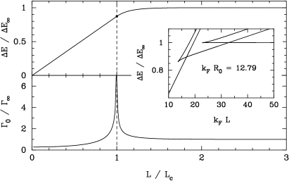
Figure 2: The activation energy $\Delta E$ as a function of the wire length $L$, for the cubic potential with Neumann boundary conditions (top). The dashed line indicates the critical wire length $L_{c}$ at which the transition takes place. The bottom panel shows the prefactor $\Gamma_{0}$, and the inset displays the activation barrier for the full potential $U(\phi)$ for $k_{F}R_{0}=12.79$, exhibiting a succession of first order phase transitions.

When the saddle is constant ($\ell\leqslant\ell_{c}$), the activation barrier scales linearly with (reduced) length $\ell$: $\Delta E/E_{0}=(4/3)\ell$. Above $\ell_{c}$, it is expressible in terms of the complete elliptic integrals of the first kind ${\bf K}(m)$ and the second kind ${\bf E}(m)$:

$$\frac{\Delta E}{E_{0}}=\left[{2-3m-3m^{2}+2m^{3}\over 3\xi(m)^{3/2}}+{2\over 3}\right]\ell\\ +{6\sqrt{2}\over 5\xi(m)^{1/4}}\left[2{\bf E}(m)-{(2-m)(1-m)\over\xi(m)}{\bf K}(m)\right]\,.$$ (13)

As $\ell\to\infty$ (corresponding to $m\to 1^{-}$), $\Delta E/E_{0}\to 12\sqrt{2}/5$. More generally, we denote the asymptotic value $\lim_{L\to\infty}\Delta E(L)\equiv\Delta E_{\infty}$. The activation barrier for the entire range of $\ell$ is shown in Fig. 2.

Calculation of the prefactor $\Gamma_{0}$ in the Kramers transition rate formula is a much more involved matter. It generally requires an analysis of the transverse fluctuations about the extremal solutions. The general method for determining $\Gamma_{0}$ has been discussed elsewhere Maier and Stein (2001); Stein (2004); here, we just present results (in units of the Debye frequency $\nu_{D}$). For $\ell<\ell_{c}$, we find

$$\Gamma_{0}^{<}={1\over\pi}{\sinh(\ell\sqrt{2})\over\sin(\ell\sqrt{2})}\,,$$ (14)

which diverges as $\ell\to{\ell_{c}}^{-}$, with a critical exponent of 1/2. The divergence arises from a soft mode; one of the eigenmodes corresponding to small fluctuations about the saddle has vanishing eigenvalue at $\ell_{c}$. This divergence, and its meaning, are discussed in detail in Stein (2004).

For $\ell>\ell_{c}$, the prefactor is

$$\Gamma_{0}^{>}={2-m+2\sqrt{4m^{2}-m+1}\over 4\pi\xi(m)^{3/8}}\\ \times\sqrt{(1-m)\sinh\Bigl{[}2\xi(m)^{1/4}{\bf K}(m)\Bigr{]}\over\xi(m){\bf E}(m)-\frac{1}{2}(1-m)(2-m){\bf K}(m)}.$$ (15)

This also exhibits a divergence with a critical exponent of $1/2$ as $\ell\to{\ell_{c}}^{+}$. The prefactor over the entire range of $\ell$ is shown in Fig. 2.

The second-order-like transition in activation behavior exhibited in Fig. 2 is interesting, but generally holds only for transitions where the potential $U(\phi)$ can be locally approximated by a smooth potential of quartic or lower order Stein (2004). For some of the minima of Fig. 1, this is not the case, and the wire instead exhibits one or more first-order-like transitions Chudnovsky (1992), as shown in the inset of Fig. 2.

Figure 3: The activation energy $\Delta E_{\infty}$ as a function of radius for a typical stable zone in Au. Solid curve: numerical result for the full potential $U(\phi)$, Eq. (6); dashed curve: result from Eq. (13) using the best cubic-polynomial fit to $U(\phi)$. The wire radius is related to the tensile stress (upper axis).

Figure 3 shows the activation barrier $\Delta E_{\infty}$ as a function of radius $\bar{R}$ for a typical metastable wire, corresponding to the conductance plateau at $G=17\,G_{0}$ in Au. Very good agreement is found between the numerical result for the full potential (6) (solid curve) and the result from Eq. (13) using the best-fit cubic polynomial $U^{(\pm)}$ (dashed curve). Under strain, $\bar{R}$ varies elastically; the corresponding stress in the wire is shown on the upper axis. A stress of a fraction of a nanonewton can significantly change the activation barrier, and even change the direction of escape. The maximum value of $\Delta E_{\infty}$ occurs at the cusp, where the activation barriers for thinning and growth are equal.

Table 1: The lifetime $\tau$ (in seconds) for various cylindrical sodium nanowires at temperatures from 75K to 125K. Here $G$ is the electrical conductance of the wire, $L_{c}$ is the critical length above which the lifetime may be approximated by $\tau\approx\nu_{D}^{-1}\exp(\Delta E_{\infty}/T)$, and $\Delta E_{\infty}$ is the activation energy for an infinitely long wire. Note that wires shorter than $L_{c}$ are predicted to have shorter lifetimes.

$G$	$L_{c}$	$\Delta E_{\infty}$	$\tau$ [s]
[$G_{0}$]	[Å]	[meV]	$75\;$K	$100\;$K	$125\;$K
3	2.8	250	$4\times 10^{5}$	2	$5\times 10^{-3}$
6	4.3	200	7	$3\times 10^{-3}$	$3\times 10^{-5}$
17	5.0	260	$7\times 10^{5}$	3	$8\times 10^{-3}$
23	6.1	230	$2\times 10^{3}$	0.2	$9\times 10^{-4}$
42	7.2	250	$2\times 10^{5}$	1	$10^{-3}$
51	6.8	190	1	$8\times 10^{-4}$	$10^{-4}$
67	18.8	180	0.6	$5\times 10^{-4}$	$7\times 10^{-6}$
96	11.4	250	$10^{5}$	0.8	$3\times 10^{-3}$

The most stable structures, corresponding to the maximum values of $\Delta E_{\infty}$, occur at (or near) the minima of the electron-shell potential, $V(R)$ (Fig. 1). The lifetimes of these equilibrated structures are limited by thinning, since the total energy of the wire is lowered by reducing its volume. We thus fit the effective potential at these minima to the form $U^{(-)}$. Table 1 lists critical lengths $L_{c}$, activation barriers $\Delta E_{\infty}$, and lifetimes $\tau=1/\Gamma$, Eq. (8), at various temperatures for Na nanowires. (Only the minima that are well-fit by $U^{(-)}$ are shown.) The temperature dependence of $\tau$ shows that the lifetime of Na nanowires drops below the threshold for observation in break-junction experiments as the temperature is increased from 75K to 125K. This behavior can explain the observed temperature dependence of conductance histograms for Na nanowires Yanson et al. (1999), which show clear peaks at conductances near the predicted values at temperatures below 100K, but were not reported at higher temperatures. The increase of $L_{c}$ with $G$, shown in Table 1, may also explain the observed exponential decrease in the heights of the conductance peaks with increasing conductance Yanson et al. (1999), since the thicker contacts are more likely to be shorter than $L_{c}$, and hence to have exponentially reduced lifetimes.

An important prediction given in Table 1 is that the lifetimes of the most stable nanowires, while they do exhibit significant variations from one conductance plateau to another, do not vary systematically as a function of radius; the activation barriers in Table 1 vary by only about 30% from one plateau to another, and the wire with a conductance of $96G_{0}$ has essentially the same lifetime as that with a conductance of $3G_{0}$. In this sense, the activation barrier is found to be universal: in any conductance interval, there are very short-lived wires (not shown in Table 1) with very small activation barriers, while the longest-lived wires have activation barriers of a universal size

$$\Delta E_{\infty}\,\simeq\,0.6\left(\frac{\hbar^{2}\sigma}{m_{e}}\right)^{1/2}\!\!\!\!\!,$$ (16)

depending only on the surface tension of the material. Here $m_{e}$ is the conduction-band effective mass, which is comparable to the free-electron rest mass. The fact that the typical activation energy (16) is independent of $\bar{R}$ is a consequence of the virial theorem: Since the instanton is a stationary state of Eq. (4), the bending energy $\langle\frac{\kappa}{2}(\partial_{z}\phi)^{2}\rangle$ is proportional to $\langle U(\phi)\rangle$. Since $\kappa\sim\sigma\bar{R}$ and $V\sim 1/\bar{R}$ Bürki et al. (2003), this implies that the characteristic size of the instanton $L_{c}\sim\sqrt{\sigma}\bar{R}$ and $\Delta E_{\infty}\sim\sqrt{\sigma}$.

Table 2: Fermi energy, surface tension, and typical critical length and activation barrier for various alkali and noble metals. The surface tension values are extrapolations to zero temperature from Ref. Tyson and Miller (1977).

Metal	Li	Na	K	Rb	Cs	Cu	Ag	Au
$\varepsilon_{F}$[eV]	4.74	3.24	2.12	1.85	1.59	7.00	5.49	5.53
$\sigma$ [N/m]	0.52	0.26	0.14	0.12	0.09	1.78	1.24	1.50
$L_{c}/\bar{R}$	0.67	0.71	0.81	0.84	0.88	0.83	0.88	0.97
$\Delta E_{\infty}$ [meV]	290	200	150	140	120	530	440	490

Table 2 lists typical activation barriers and critical lengths for various alkali and noble metals. It shows that noble metal nanowires should have much longer lifetimes than alkali metal nanowires, due to their larger surface tension coefficients. This prediction is consistent with experimental observations Kondo and Takayanagi (1997); Rodrigues et al. (2002); Oshima et al. (2003); Smit et al. (2004); Yanson et al. (1999, 2001), although our estimated activation barriers for noble metal nanowires are still too small to account for their observed stability at room temperature. This discrepancy may stem from the neglect of $d$-electrons in our model (except inasmuch as they enhance $\sigma$ compared to the free-electron value), or due to the presence of impurities which passivate the surface, thereby raising the activation barrier above its intrinsic value.