Data collapse in the critical region using finite-size scaling with subleading corrections

Abstract

We propose a treatment of the subleading corrections to finite-size scaling that preserves the notion of data collapse. This approach is used to extend and improve the usual Binder cumulant analysis. As a demonstration, we present results for the two- and three-dimensional classical Ising models and the two-dimensional, double-layer quantum antiferromagnet.

True phase transitions occur only in systems with an infinite number of degrees of freedom. Nevertheless, it is possible to study critical phenomena by simulating finite systems of increasing size and extrapolating their behaviour to the thermodynamic limit. The standard analysis relies on Fisher’s finite-size scaling (FSS) hypothesis Fisher71 ; Fisher72 , which supposes that near a critical point every thermodynamic property of the system scales as a universal function of the ratio $L/\xi$, where $L$ is the linear size of the system and $\xi$ is the bulk correlation length.

The basic ansatz is that any property with critical exponent $\kappa$ obeys the relation $A(T,L)=L^{\kappa/\nu}f_{A}(L/\xi(t))$, which is valid for large $L$ and small reduced temperature $t=(T-{T}_{\text{c}})/{T}_{\text{c}}$. Here, ${T}_{\text{c}}$ is the critical temperature of the transition, and $\nu$ is the critical exponent of the correlation length $\xi\sim\lvert t\rvert^{-\nu}$. The function $f_{A}(x)$ depends only on the boundary conditions and the system geometry. Equivalently, one can write

$$A(T,L)L^{-\kappa/\nu}=g_{A}(tL^{1/\nu}).$$ (1)

Equation (1) can be formally motivated Brezin82 ; Barber83 ; Brezin85 by arguing that the diverging correlation length leaves the system scale invariant Stanley99 . As $t\rightarrow 0$, fluctuations of the dynamical variables begin to look the same on all length scales (much greater than the lattice spacing). Consequently, any change in the system size $L$ can be compensated by a corresponding change in temperature $t$. The two otherwise independent quantities become locked together in a single composite variable $x=tL^{1/\nu}$.

Graphically, this effect is undersood in terms of so-called data collapse Binder70_80 ; Ferron04 . A plot of Eq. (1) in reduced variables traces out the universal function $g_{A}(x)$. Such a plot can be useful as a data analysis tool. Given some set of measurements $\{(T_{i},L_{i},A_{i})\}$, the critical behaviour of the system can be determined by constructing the coordinates $x_{i}=L_{i}^{1/\nu}(T_{i}-{T}_{\text{c}})/{T}_{\text{c}}$ and $y_{i}=A_{i}L_{i}^{-\kappa/\nu}$ and choosing the values of $\nu$, $\kappa$, and ${T}_{\text{c}}$ such that the graph points $\{(x_{i},y_{i})\}$ have the least amount of scatter endnote1 .

The accuracy of such a fit depends not only on the quantity and quality of the data; it also depends sensitively on whether the data are sufficiently deep in the scaling limit ($L\rightarrow\infty$ at fixed $x$). What constitutes “deep enough,” however, is model dependent and difficult to determine. For high-accuracy studies, it is best not to put complete trust in Eq. (1). Since true scaling is realized only asymptotically, data from all but the largest systems can rarely be made to fall onto a single curve. Worse, the data can sometimes be shoehorned into collapse with incorrect parameters. For lattice sizes that are accessible to computer simulation, there are almost always significant, non-universal corrections to FSS. To simply ignore them can lead to subtle systematic errors, unreliable fits, and overly-optimistic error estimates.

In this Letter, we show how to incorporate subleading corrections into the minimal-scatter optimization described above. We argue that the correct approach is to make small, size-dependent modifications to the prefactor and argument of $g_{A}(x)$ in Eq. (1):

$$A(T,L)L^{-\kappa/\nu}=\mathcal{N}(L)g_{A}(tL^{1/\nu}-\epsilon(L)).$$ (2)

In other words, the features of $A$ are both renormalized and shifted. In the thermodynamic limit, $\mathcal{N}(L)\rightarrow 1$ and $\epsilon(L)\rightarrow 0$; we determine the precise asymptotic form of these functions by renormalization group arguments. The key point is that $\tilde{y}=A(T,L)L^{-\kappa/\nu}\mathcal{N}(L)^{-1}$ now behaves as a universal function of $\tilde{x}=tL^{1/\nu}-\epsilon(L)$.

In the special case where $g_{A}(x)$ is bounded and monotonic, $A(T,L)L^{-\kappa/\nu}$ becomes increasingly step-function-like as $L\rightarrow\infty$. Thus, two such curves, plotted versus temperature for different linear sizes $L$ and $L^{\prime}$, will intersect (except in unusual circumstances) at a unique point in the vicinity of the critical temperature ${T}_{\text{c}}$. Binder’s spin-distribution cumulants Binder81 have this useful property (as does, e.g., the spin stiffness Wang05 ). In the Binder cumulant case, $\kappa=0$ happens to be known a priori. We solve formally for the point of intersection ${T}_{\text{i}}(L,L^{\prime})$ under the assumption of Eq. (2)-like scaling and determine its location as a function of $L$ and $n=L^{\prime}/L$. We prove that a sequence of intersection points ($n$ fixed, $L\rightarrow\infty$) converges to ${T}_{\text{c}}$ faster than $L^{-1/\nu}$. Fitting the $n$ dependence of a data set offers another way of estimating ${T}_{\text{c}}$ and $\nu$.

Corrections to finite-size scaling—FSS can be put on a (somewhat) rigourous basis by invoking the renormalization group (RG) Brezin82 ; Barber83 ; Brezin85 . From the RG point of view, the system is characterized by a set of scaling fields $\{\zeta_{i}\}$. The singular part of the free energy behaves according to

$$f_{\text{s}}(\zeta_{1},\zeta_{2},\zeta_{3},\ldots)=L^{-d}\mathcal{F}(\zeta_{1}L^{y_{1}},\zeta_{2}L^{y_{2}},\zeta_{3}L^{y_{3}},\ldots),$$ (3)

where $\mathcal{F}(x_{1},x_{2},x_{3},\ldots)$ is a regular function of its arguments. The $y_{i}$ are eigenvalues of the RG transformation and characterize the flow of the fields under the rescaling $L\mapsto L/b$ with $b>1$; i.e., $\zeta_{i}\mapsto\zeta_{i}b^{y_{i}}$.

For concreteness, suppose that there is only one relevant scaling field $\zeta_{1}=t$ with a scaling exponent $y_{1}=1/\nu>0$. Then $f_{\text{s}}$ admits a series expansion in the remaining fields (with $\zeta_{i}=\zeta_{i,0}$ fixed):

$$f_{\text{s}}\!=\!L^{-d}\prod_{i=2}^{\infty}\sum_{n=0}^{\infty}\frac{\zeta_{i,0}^{n}L^{-n\lvert y_{i}\rvert}}{n!}\frac{\partial^{n}}{\partial x_{i}^{n}}\mathcal{F}(tL^{1/\nu}\!,x_{2},x_{3},\ldots)\biggr{\rvert}_{x_{i}=0}.$$ (4)

It follows that any thermodynamic quantity generated from Eq. (4) will have the form

$$A(T,L)=L^{\kappa/\nu}g_{A}(tL^{1/\nu})+L^{(\kappa-\phi)/\nu}p_{A}(tL^{1/\nu})+\cdots$$ (5)

where $\phi/\nu=\min(\lvert y_{i}\rvert)$. The functions $g_{A}(x)$ and $p_{A}(x)$ are partial derivatives of $\mathcal{F}$. Their asymptotic behaviour, $g_{A}(x)\sim\lvert x\rvert^{-\kappa}$ and $p_{A}(x)\sim\lvert x\rvert^{-\kappa+\phi}$ as $x\rightarrow\pm\infty$, leads to the thermodynamic limit

$$A(T)=\lim_{L\rightarrow\infty}A(T,L)\sim\lvert t\rvert^{\kappa}\bigl{(}1+(\text{const})\lvert t\rvert^{\phi}+\cdots\bigr{)}.$$ (6)

The functions $g_{A}(x)$ and $p_{A}(x)$ are well-behaved and admit series expansions $g_{A}(x)=g_{0}+g_{1}x+\frac{1}{2}g_{2}x^{2}+\cdots$, etc. Identifying Eqs. (2) and (5) up to $O(x^{3})$, we find that $\mathcal{N}(L)=1+C_{1}L^{-\phi/\nu}$ and $\epsilon(L)=C_{2}L^{-\phi/\nu}$, where

$$C_{1}=\frac{g_{2}p_{0}-g_{1}p_{1}}{g_{2}g_{0}-g_{1}^{2}}\ \ \text{and}\ \ C_{2}=\frac{g_{0}p_{1}-g_{1}p_{0}}{g_{2}g_{0}-g_{1}^{2}}.$$ (7)

This analysis is flawed, however, in that scaling holds only asymptotically. The “equalities” in Eqs. (3) and (4) are subject to corrections analytic in $L^{-1}$. This means that, strictly speaking, $\mathcal{N}(L)=(1+C_{1}L^{-\phi/\nu}+\cdots)(1+a_{1}L^{-1}+a_{2}L^{-2}+\cdots)$. Over some range of $L$ values, this can be represented by $\mathcal{N}(L)=1+cL^{-\omega}$, where $\omega$ has some effective value close to that of the true $L\rightarrow\infty$ exponent, $\min(\phi/\nu,1)$. Thus,

$$A(T,L)=L^{\kappa/\nu}\bigl{(}1+cL^{-\omega})g_{A}(tL^{1/\nu}-dL^{-\phi/\nu})$$ (8)

is the appropriate generalization of Eq. (1). Most important, this scaling ansatz represents an improvement over Eq. (5) in that data collapse can still be engineered by plotting $AL^{-\kappa/\nu}(1+cL^{-\omega})^{-1}$ versus $tL^{1/\nu}-dL^{-\phi/\nu}$, with the addition of $\omega$, $\phi$, $c$, and $d$ as fitting parameters.

Intersection point analysis—In the vicinity of a magnetic phase transition, expectation values of powers of the magnetization obey the scaling relation $\langle\lvert M\rvert^{p}\rangle_{L}=L^{-p\beta/\nu}g_{|\!M\!|^{p}}(tL^{1/\nu})$ for integer $p>0$. At large $x$, the scaling function $g_{|\!M\!|^{p}}(x)$ exhibits power-law behaviour with exponents $p\beta$ as $x\rightarrow-\infty$ and $p\tilde{\beta}<p\beta$ as $x\rightarrow\infty$, which ensures that the magnetization has the correct form in the thermodynamic limit: $\langle\lvert M\rvert^{p}\rangle_{\infty}=(-t)^{p\beta}\theta(-t).$ One can define a family of quotient functions Binder81

$$Q_{p}(T,L)=\frac{\langle M^{2p}\rangle_{L}}{\langle M^{2}\rangle_{L}^{p}}=\mathcal{N}(L)q_{p}(tL^{1/\nu}-\epsilon(L))$$ (9)

—let us call them Binder ratios—constructed in such a way that the leading-order $L$ dependence outside the scaling function factors out. The temperature dependence appears only in the argument of the function $q_{p}(x)=g_{M^{2p}}(x)/[g_{M^{2}}(x)]^{p}$. The subleading corrections enter as shown on the right-hand side of Eq. (9). The two lowest order Binder cumulants [Eqs. (11) and (12) of Ref. Binder81, ] correspond to the linear combinations $U=1-\tfrac{1}{3}Q_{2}$ and $V=1-\tfrac{1}{2}Q_{2}+\tfrac{1}{30}Q_{3}$.

In the thermodynamic limit, the Binder ratios jump discontinuously between $Q_{p}(T<{T}_{\text{c}})=q_{p}(-\infty)=1$ and $Q_{p}(T>{T}_{\text{c}})=q_{p}(\infty)$. The value of $q_{p}(\infty)\neq 1$ is simply a prefactor of the gaussian distribution of thermally randomize spins; the value $Q_{p}({T}_{\text{c}})=q_{p}(0)$ is a non-trivial, universal constant. The Binder cumulants are also step functions, taking the values $U=2/3$ and $V=8/15$ in the ordered phase and $U=V=0$ in the disordered phase.

We now consider the point of intersection ${T}_{\text{i}}(L,L^{\prime})$ between two Binder ratio curves for system sizes $L\neq L^{\prime}$. To start, let us assume that ${T}_{\text{i}}(L,nL)$, for some fixed ratio $n=L^{\prime}/L$, converges to ${T}_{\text{c}}$ as a function of $L$ faster than $L^{-1/\nu}$. In that case, ${t}_{\text{i}}(L,nL)L^{1/\nu}$ is a small quantity. Accordingly,

$$Q({T}_{\text{i}},L)=\mathcal{N}(L)\Bigl{[}q_{0}+q_{1}\bigl{(}{t}_{\text{i}}L^{1/\nu}-\epsilon(L)\bigr{)}+\cdots\Bigr{]}.$$ (10)

[We have dropped the $p$ label; the subscripts here refer to the expansion coefficients of $q(x)$ about $x=0$.] Hence, the crossing criterion $Q({T}_{\text{i}},L)=Q({T}_{\text{i}},L^{\prime})$ implies that

$${t}_{\text{i}}=\frac{-q_{0}\bigl{[}\mathcal{N}(L)-\mathcal{N}(L^{\prime})\bigr{]}+q_{1}\bigl{[}\mathcal{N}(L)\epsilon(L)-\mathcal{N}(L^{\prime})\epsilon(L^{\prime})\bigr{]}}{q_{1}\bigl{[}\mathcal{N}(L)L^{1/\nu}-\mathcal{N}(L^{\prime})(L^{\prime})^{1/\nu}\bigr{]}}$$ (11)

or, in the notation of Eq. (8),

$${t}_{\text{i}}(L,nL)=\frac{cq_{0}}{q_{1}}\biggl{(}\frac{1-n^{-\omega}}{n^{1/\nu}-1}\biggr{)}L^{-1/\nu-\omega}\\ -d\biggl{(}\frac{1-n^{-\phi/\nu}}{n^{1/\nu}-1}\biggr{)}L^{-(1+\phi)/\nu}.$$ (12)

[In retrospect, the assumption that ${T}_{\text{i}}(L,nL)\rightarrow{T}_{\text{c}}$ faster than $L^{-1/\nu}$ was justified.] Note that although Eq. (12) was derived with the Binder ratio in mind, it applies equally to any quantity $A(T,L)L^{-\kappa/\nu}$ obeying Eq. (8) whose scaling function is bounded and monotonic.

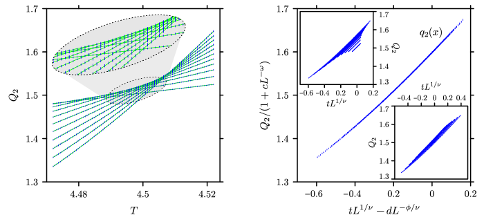
Figure 1: (color online) The second Binder ratio $Q_{2}(T,L)$, computed via Monte Carlo for the 3D Ising model on lattices of size $L=4,5,\ldots,14$. In the left-hand panel, the solid (green) lines are guides to the eye, connecting data points computed for equal system sizes; the curves grow steeper with increasing $L$. The oval inset presents a magnified view in which the individual data points and their error bars (blue) are more clearly visible. The scaling plot in the right-hand panel shows the complete collapse of the data onto a single curve. This best fit gives ${T}_{\text{c}}=4.5114(2)$, $\nu=0.625(1)$, and $q_{2}(0)=1.60(1)$ [or $U^{*}=1-\frac{1}{3}q_{2}(0)$ = 0.467(3)]. The two inset panels are purely leading-order scaling plots ($c=d=0$) based on (top-left) the best fit values just quoted and (bottom-right) the values ${T}_{\text{c}}=4.500(2)$, $\nu=0.60(1)$ obtained by fitting $Q_{2}$ versus $tL^{1/\nu}$.

Numerical results—We have applied these results to three numerical test cases: the two- (2D) and three-dimensional (3D) nearest-neighbour Ising models, and the double-layer quantum Heisenberg antiferromagnet Shevchenko00 . Monte Carlo data were generated for the Ising models using the Swendsen-Wang cluster update algorithm Swendsen87 and for the quantum antiferromagnet using stochastic series expansion Sandvik99 .

The Ising models exhibit classical, thermally-driven phase transitions at $T_{\text{c,2D}}=2/\log(1+\sqrt{2})\approx 2.2691853$ and $T_{\text{c,3D}}\approx 4.511$. The antiferromagnetic bilayer, on the other hand, exhibits a zero-temperature, quantum phase transition as the interlayer coupling strength $\alpha$ is tuned through its critical value ${\alpha}_{\text{c}}\approx 2.5218$ Shevchenko00 ; Wang05 . For each of these cases, we computed the second Binder ratio over a fine, uniform mesh of temperature (coupling) values in a fixed interval containing ${T}_{\text{c}}$ (${\alpha}_{\text{c}}$). (In practice, when rough estimates of ${T}_{\text{c}}$ and $\nu$ are available in advance, it makes more sense to take measurements in the range $\lvert x\rvert=\lvert t\rvert L^{1/\nu}\lesssim 1$.) The simulations were performed for a range of relatively small lattice sizes.

The data were fit to Eq. (8) (with $\kappa=0$) using the the Levenberg-Marquardt nonlinear optimization algorithm Gill81 , which searched the space of parameters ${T}_{\text{c}}$ (${\alpha}_{\text{c}}$), $\nu$, $\omega$, $\phi$, $c$, and $d$ to produce the best collapse of the data. Uncertainties in those values were computed by bootstrapping Efron93 the regression over the original Monte Carlo data. Comparison with the 2D Ising model, where the solution is known Onsager44 , serves as an important proof of concept: the fitted values ${T}_{\text{c}}=2.26917(2)$ and $\nu=0.99(1)$ with $L=4,5,\ldots,32$ agree within statistical uncertainties with the exact results. The same procedure applied to the quantum bilayer with $L=8,10,12,\ldots,42$ yields ${\alpha}_{\text{c}}=2.52181(4)$, the most accurate value to date, and $\nu=0.715(2)$, which is consistent with the 3D classical Heisenberg universality class, as expected Chakravarty88 .

The raw data for the 3D Ising model are shown in the left-hand panel of Fig. 1. In the right-hand panel, the same data are rescaled according to Eq. (8) and collapse convincingly onto a single curve. The two inset panels on the right illustrate the failure of naive FSS: plotted in the conventional reduced coordinates ($c=d=0$), the data are clearly distinguishable as a series of separate curves corresponding to different lattice sizes.

The fitted value of the critical temperature ${T}_{\text{c}}=4.5114(2)$ is consistent with the Rosengren conjecture Rosengren86 and with other reliable estimates; cf. Ref. Talapov96, and Table 19 in Ref. Blote95, . Note that our result is nearly as accurate as those of Pawley et al. and Garcia et al. (viz., ${T}_{\text{c}}=4.5115(1)$ in Ref. Pawley84, and ${T}_{\text{c}}=4.51152(12)$ in Ref. Garcia03, ), which are based on simulations up to sizes $L=64$ and $L=115$, respectively. And while our value of $\nu=0.625(1)$ is small with respect to some estimates Pawley84 ; Ferrenberg91 ; Blote95 , it appears to be in very good agreement with more recent Monte Carlo ($L=90,100,115$) Garcia03 and Monte Carlo Renormalization Group ($L=64,128,256$) Baillie92 ; Gupta96 calculations. As an additional check, we can read off the value $q_{2}(0)=1.60(1)$ (the “y-intercept” in the right-hand panel of Fig. 1), which agrees with the value $q_{2}(0)=1.604(1)$ computed by independent methods Blote95 .

Figure 2 plots the Binder ratio intersection points of the 2D Ising model and the quantum bilayer for several system size ratios $n=L^{\prime}/L$. In each case, the complete set of crossing points was computed by interpolating smooth curves between the measured $Q_{2}$ values (as in the left panel of Fig. 1, where the grid lines form a set of intersection points). The data were successfully fit to the scaling form given by Eqs. (11) and (12). The resulting estimates ${T}_{\text{c}}=2.2692(8)$, $\nu=0.99(2)$ and ${\alpha}_{\text{c}}=2.5218(2)$, $\nu=0.715(8)$ are somewhat less accurate than but consistent with the values determined by the data collapse analysis.

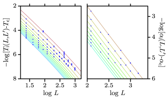
Figure 2: (color online) Binder ratio crossing points ${T}_{\text{i}}(L,L^{\prime})$ plotted with respect to $L$ ($<L^{\prime}$) for the (left) 2D Ising model and (right) double-layer quantum antiferromagnet. The solid lines depict the analytic result given in Eq. (12) for lines of constant $n=L^{\prime}/L$. From top (red) to bottom (blue), the ratios shown are (left) $n=8/7$, $n=3/2,2,\ldots,11/2,6$ (by increments of $1/2$) and (right) $n=3/2,2,\ldots,9/2,5$.

Conclusions—Finite-size scaling describes how critical behaviour emerges from finite systems in the limit of increasingly large system size. As $L\rightarrow\infty$, quantities in the critical region become universal modulo a size-dependent rescaling of the variables, a property which, in principle, can be exploited to measure unknown critical parameters by means of data collapse. In practice, such an analysis is likely to give misleading results. Still, we have shown that data collapse can be made a viable, high-accuracy analysis tool, so long as subleading corrections to finite-size scaling are properly taken into account. We have introduced a new way of expressing those corrections, in which two kinds of deformation—the renormalization $g_{A}\rightarrow\mathcal{N}g_{A}$ and the shift $g_{A}(x)\rightarrow g_{A}(x-\epsilon)$—serve as the fundamental deviations from leading-order FSS. The greater expressiveness of the scaling form typically leads to larger but more meaningful and reliable statistical errors on the critical parameters.

Large simulations devour computing resources. With Monte Carlo, CPU time scales as $L^{d+z}$, where $z$ is a characteristic dynamical exponent. For the Ising model in $d=3$, Swendsen-Wang updates Swendsen87 give $z\approx 0.75$. This implies that it takes as much time to compute the single system size $L=16$ as it does to compute all of $L=4,5,\ldots,12$. (Even worse, for models where specialized update schemes are not available, $z\approx 2$.) The success of Eq. (8) as a fitting form well away from the scaling limit has an interesting implication: it may be more profitable to collect a large quantity of easily-obtainable intermediate-$L$ data endnote2 (so as to maximize the fit statistics) than to make a herculean effort to obtain data for the very largest possible lattice sizes.

References

- (1) M. E. Fisher, in Critical Phenomena, Proceedings of the Enrico Fermi International School of Physics, ed. M. S. Green (Academic, New York, 1971), Vol. 51.
- (2) M. E. Fisher and M. N. Barber, Phys. Rev. Lett., 28, 1516 (1972).
- (3) E. Brézin, J. Phys. (Paris) 43, 15 (1982).
- (4) M. N. Barber, in Phase Transitions and Critical Phenomena, ed. C. Domb (Academic, New York, 1983), Vol. 8.
- (5) E. Brézin and J. Zinn-Justin, Nucl. Phys. B 257, 867 (1985).
- (6) H. E. Stanley, Rev. Mod. Phys. 71, S358 (1999).
- (7) K. Binder, Thin Solid Films 20, 367 (1974); D. P. Landau, Phys. Rev. B 13, 2997 (1976); K. Binder and D. P. Landau, ibid. 21, 1941 (1980).
- (8) A. Ferrón and P. Serra, J. Chem. Phys. 120, 8412 (2004).
- (9) A suitable goodness of fit measure for data collapse can be defined even with no knowledge of ; see S. M. Bhattacharjee and F. Seno, J. Phys. A 34, 6375 (2001).
- (10) K. Binder, Z. Phys. B 43, 119-140 (1981).
- (11) L. Wang, K. S. D. Beach, A. W. Sandvik, to be published.
- (12) P. V. Shevchenko, A. W. Sandvik, and O. P. Sushkov, Phys. Rev. B 61, 3475 (2000).
- (13) R. H. Swendsen and J.-S. Wang, Phys. Rev. Lett. 58, 86 (1987).
- (14) A. Sandvik, Phys. Rev. B, 59, R14157 (1999); ibid. 56, 11678 (1997).
- (15) P. R. Gill, W. Murray, and M. H. Wright, Practical Optimization (Academic Press, San Diego, 1988).
- (16) B. Efron and R. Tibshirani, An Introduction to the Bootstrap (Chapman & Hall/CRC, Boca Raton, 1993).
- (17) L. Onsager, Phys. Rev. 65, 117 (1944).
- (18) S. Chakravarty, B. I. Halperin, and D. R. Nelson, Phys. Rev. Lett. 60, 1057 (1988).
- (19) A. Rosengren, J. Phys. A 19, 1709 (1986).
- (20) A. L. Talapov and H. W. J. Blöte, J. Phys. A 29, 5727 (1996); cond-mat/9603013
- (21) H. W. J. Blöte, E. Luijten, and J. R. Herniga, J. Phys. A 28, 6289 (1995).
- (22) G. S. Pawley, R. H. Swendsen, D. J. Wallace, K. G. Wilson, Phys. Rev. B 29, 4030 (1984).
- (23) J. Garcia and J. A. Gonzalo, Physica A 326, 464 (2003); cond-mat/0211270
- (24) A. M. Ferrenberg and D. P. Landau, Phys. Rev. B 44, 5081 (1991).
- (25) C. F. Baillie, R. Gupta, K. A. Hawick, and G. S. Pawley, Phys. Rev. B 45, 10438 (1992).
- (26) R. Gupta and P. Tamayo, Int. J. Mod. Phys. C 7, 305 (1996); cond-mat/9601048
- (27) Some care must be taken. There may be a crossover scale such that corresponds to an entirely different universality class.