Characterization of Complex Networks:
A Survey of measurements

Abstract

Each complex network (or class of networks) presents specific topological features which characterize its connectivity and highly influence the dynamics of processes executed on the network. The analysis, discrimination, and synthesis of complex networks therefore rely on the use of measurements capable of expressing the most relevant topological features. This article presents a survey of such measurements. It includes general considerations about complex network characterization, a brief review of the principal models, and the presentation of the main existing measurements. Important related issues covered in this work comprise the representation of the evolution of complex networks in terms of trajectories in several measurement spaces, the analysis of the correlations between some of the most traditional measurements, perturbation analysis, as well as the use of multivariate statistics for feature selection and network classification. Depending on the network and the analysis task one has in mind, a specific set of features may be chosen. It is hoped that the present survey will help the proper application and interpretation of measurements.

1 Introduction

Complex networks research can be conceptualized as lying at the intersection between graph theory and statistical mechanics, which endows it with a truly multidisciplinary nature. While its origin can be traced back to the pioneering works on percolation and random graphs by Flory [1], Rapoport [2, 3, 4], and Erdős and Rényi [5, 6, 7], research in complex networks became a focus of attention only recently. The main reason for this was the discovery that real networks have characteristics which are not explained by uniformly random connectivity. Instead, networks derived from real data may involve community structure, power law degree distributions and hubs, among other structural features. Three particular developments have contributed particularly for the ongoing related developments: Watts and Strogatz’s investigation of small-world networks [8], Barabási and Albert’s characterization of scale-free models [9], and Girvan and Newman’s identification of the community structures present in many networks (e.g. [10]).

Although graph theory is a well-established and developed area in mathematics and theoretical computer science (e.g., [11, 12]), many of the recent developments in complex networks have taken place in areas such as sociology (e.g., [13, 14]), biology (e.g., [15]) and physics (e.g., [16, 17]). Current interest has focused not only on applying the developed concepts to many real data and situations, but also on studying the dynamical evolution of network topology. Supported by the availability of high performance computers and large data collections, results like the discovery of the scale-free structure of the Internet [18] and of the WWW [19, 20] were of major importance for the increased interest on the new area of complex networks, whose growing relevance has been substantiated by a large number of recent related publications. Reviews of such developments have been presented in four excellent surveys [21, 22, 23, 24], introductory papers [25, 26, 27, 17] and several books [28, 29, 13, 30, 31, 16, 32]. For additional information about the related areas of percolation, disordered systems and fractals see [33, 34, 35]; for complex systems, see [36, 37, 38].

One of the main reasons behind complex networks popularity is their flexibility and generality for representing virtually any natural structure, including those undergoing dynamical changes of topology. As a matter of fact, every discrete structure such as lists, trees, or even lattices, can be suitably represented as special cases of graphs. It is thus little surprising that several investigations in complex network involve the representation of the structure of interest as a network, followed by an analysis of the topological features of the obtained representation performed in terms of a set of informative measurements. Another interesting problem consists of measuring the structural properties of evolving networks in order to characterize how the connectivity of the investigated structures changes along the process. Both such activities can be understood as directed to the topological characterization of the studied structures. Another related application is to use the obtained measurements in order to identify different categories of structures, which is directly related to the area of pattern recognition [39, 40]. Even when modeling networks, it is often necessary to compare the realizations of the model with real networks, which can be done in terms of the respective measurements. Provided the measurements are comprehensive (ideally the representation by the measurements should be one-to-one or invertible), the fact that the simulated networks yield measurements similar to those of the real counterparts supports the validity of the model.

Particular attention has recently been focused on the relationship between the structure and dynamics of complex networks, an issue which has been covered in two excellent comprehensive reviews [21, 23]. However, relatively little attention has been given to the also important subject of network measurements (e.g. [41]). Indeed, it is only by obtaining informative quantitative features of the networks topology that they can be characterized and analyzed and, particularly, their structure can be fully related with the respective dynamics. The quantitative description of the networks properties also provides fundamental subsidies for classifying theoretical and real networks into major categories. The present survey main objective is to provide a comprehensive and accessible review of the main measurements which can be used in to quantify important properties of complex networks.

Network measurements are therefore essential as a direct or subsidiary resource in many network investigations, including representation, characterization, classification and modeling. Figure 1 shows the mapping of a generic complex network into the feature vector $\vec{\mu}$, i.e. a vector of related measurements such as average vertex degree, average clustering coefficient, the network diameter, and so on. In case the mapping is invertible, in the sense that the network can be recovered from the feature vector, the mapping is said to provide a representation of the network. An example of invertible mapping for networks with uniform vertices and edges is the adjacency matrix (see 2). Note, however, that the characterization and classification of networks does not necessarily require invertible measurements. An interesting strategy which can be used to obtain additional information about the structure of complex networks involves applying a transformation to the original network and obtaining the measurements from the resulting network, as illustrated in Figure 2. In this figure, a transformation $T$ (in this case, deletion of the vertices adjacent to just one other vertex) is applied over the original network to obtain a transformed structure from which new measurements $\vec{\mu}_{T}$ are extracted. In case the feature vectors $\vec{\mu}$ and ${\vec{\mu}_{T}}$ correspond to the same set of measurements, it is also possible to consider the difference between these two vectors in order to obtain additional information about the network under analysis.

Perturbations of networks, which can be understood as a special case of the transformation framework outlined above, can also be used to investigate the sensitivity of the measurements. Informally speaking, if the measurements considered in the feature vector are such that small changes of the network topology (e.g., add/remove a few edges or vertices) imply large changes in the measurements (large values of $||\Delta\vec{\mu}||$), those measurements can be considered as being highly sensitive or unstable. One example of such an unstable measurement is the average shortest path length between two vertices (see Section 16.2).

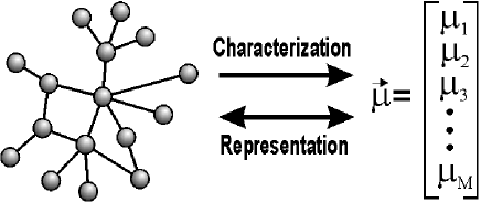
Figure 1: The mapping from a complex network into a feature vector. Generic mappings can be used in order to obtain the characterization of the network in terms of a suitable set of measurements. In case the mapping is invertible, we have a complete representation of the original structure.

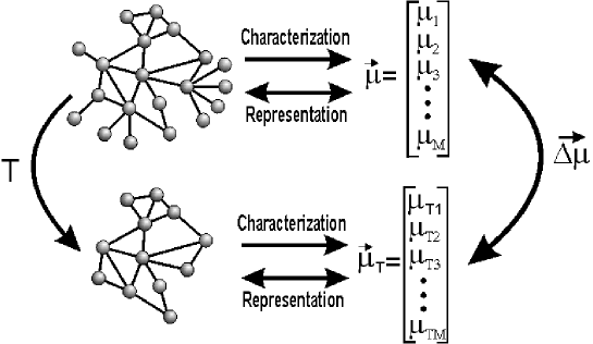
Figure 2: Additional measurements of a complex network can be obtained by applying a transformation $T$ on it and obtaining a new feature vector $\vec{\mu}_{T}$. The difference $\Delta\vec{\mu}$ between the original and transformed features vectors can also be considered in order to obtain additional insights about the properties of the original network.

Another possibility to obtain a richer set of measurements involves the consideration of several instances along development/growth of the network. A feature vector $\vec{\mu}(t)$ is obtained at each “time” instant $t$ along the growth. Figure 3 shows four instances of an evolving network and the respective trajectory defined in one of the possible feature (or phase) spaces involving two generic measurements $\mu_{1}$ and $\mu_{2}$. In such a way, the evolution of a network can now be investigated in terms of a trajectory in a features space.

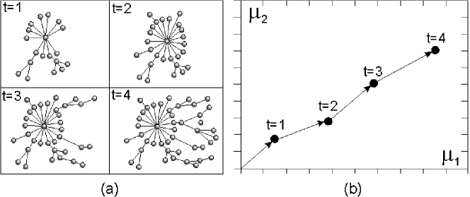
Figure 3: Given a network undergoing some dynamical evolution (a) and a set of measurements (e.g., $\mu_{1}$ and $\mu_{2}$), trajectories can be defined in the feature space (b).

Both the characterization and classification of natural and human-made structures using complex networks imply the same important question of how to choose the most appropriate measurements. While such a choice should reflect the specific interests and application, it is unfortunate that there is no mathematical procedure for identifying the best measurements. There is an unlimited set of topological measurements, and they are often correlated, implying redundancy. Statistical approaches to decorrelation (e.g., principal component analysis and canonical analysis) can help select and enhance measurements (see Section 18), but are not guaranteed to produce optimal results (e.g [39]). Ultimately, one has to rely on her/his knowledge of the problem and available measurements in order to select a suitable set of features to be considered. For such reasons, it is of paramount importance to have a good knowledge not only of the most representative measurements, but also of their respective properties and interpretation. Although a small number of topological measurements, namely the average vertex degree, clustering coefficient and average shortest path length, were typically considered for complex network characterization during the initial stages of this area, a series of new and more sophisticated features have been proposed and used in the literature along the last years. Actually, the fast pace of developments and new results reported in this very dynamic area makes it particularly difficult to follow and to organize the existing measurements.

This review starts by presenting the basic concepts and notation in complex networks and follows by presenting several topological measurements. Illustrations of some of these measurements respectively to Erdős-Rényi, Watts-Strogatz, Barabási-Albert, modular and geographical models are also included. The measurements are presented in sections organized according to their main types, including distance-based measurements, clustering coefficients, assortativity, entropies, centrality, subgraphs, spectral analysis, community-based measurements, hierarchical measurements, and fractal dimensions. A representative set of such measurements is applied to the five considered models and the results are presented and discussed in terms of their cross-correlations and trajectories. The important subjects of measurement selection and assignment of categories to given complex networks are then covered from the light of formal multivariate pattern recognition, including the illustration of such a possibility by using canonical projections and Bayesian decision theory.

2 Basic Concepts

Figure 4 shows the four main types of complex networks, which include weighted digraphs (directed graphs), unweighted digraphs, weighted graphs and unweighted graphs. The operation of symmetry can be used to transform a digraph into a graph, and the operation of thresholding can be applied to transform a weighted graph into its unweighted counterpart. These types of graphs and operations are defined more formally in the following, starting from the concept of weighted digraph, from which all the other three types can be derived.

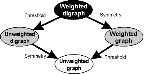
Figure 4: The four main types of complex networks and their transformations. All network types can be derived from the weighted digraph through appropriate transformations.

A weighted directed graph, $G$, is defined by a set $\mathcal{N}(G)$ of $N$ vertices (or nodes), a set $\mathcal{E}(G)$ of $M$ edges (or links), and a mapping $\omega:\mathcal{E}(G)\mapsto\mathbb{R}$. Each vertex can be identified by an integer value $i=1,2,\ldots,N$; the edges are identified by a pair $(i,j)$ that represents a connection going from vertex $i$ to vertex $j$ to which a weight $\omega(i,j)$ is associated. In the complex network literature, it is often assumed that no self-connections or multiple connections exist; i.e. there are no edges of the form $(i,i)$ and for each pair of edges $(i_{1},j_{1})$ and $(i_{2},j_{2})$ it holds that $i_{1}\neq i_{2}$ or $j_{1}\neq j_{2}$. Graphs with self- or duplicate connections are sometimes called multigraphs, or degenerate graphs. Only non-degenerate graphs are considered henceforth. In an unweighted digraph, the edges have no weight, and the mapping $\omega$ is not needed. For undirected graphs (weighted or unweighted), the edges have no directions; the presence of a edge $(i,j)$ in $\mathcal{E}(G)$ thus means that a connection exist from $i$ to $j$ and from $j$ to $i$.

A weighted digraph can be completely represented in terms of its weight matrix $W$, so that each element $w_{ij}=\omega(i,j)$ expresses the weight of the connection from vertex $i$ to vertex $j$. The operation of thresholding can be applied to a weighted digraph to produce an unweighted counterpart. This operation, henceforth represented as $\delta_{T}(W)$, is applied to each element of the matrix $W$, yielding the matrix $A=\delta_{T}(W)$. The elements of the matrix $A$ are computed comparing the corresponding elements of $W$ with a specified threshold $T$; in case $|w_{ij}|>T$ we have $a_{ij}=1$, otherwise $a_{ij}=0$. The resulting matrix $A$ can be understood as the adjacency matrix of the unweighted digraph obtained as a result of the thresholding operation. Any weighted digraph can be transformed into a graph by using the symmetry operation $\sigma(W)=W+W^{T}$, where $W^{T}$ is the transpose of $W$.

For undirected graphs, two vertices $i$ and $j$ are said to be adjacent or neighbors if $a_{ij}\neq 0$. For directed graphs, the corresponding concepts are those of predecessor and successor: if $a_{ij}\neq 0$ then $i$ is a predecessor of $j$ and $j$ is a successor of $i$. The concept of adjacency can also be used in digraphs by considering predecessors and successors as adjacent vertices. The neighborhood of a vertex $i$, henceforth represented as $\nu(i)$, corresponds to the set of vertices adjacent to $i$.

The degree of a vertex $i$, hence $k_{i}$, is the number of edges connected to that vertex, i.e. the cardinality of the set $\nu(i)$ (in the physics literature, this quantity is often called “connectivity” [22]). For undirected networks it can be computed as

$$k_{i}=\sum_{j}a_{ij}=\sum_{j}a_{ji}.$$ (1)

The average degree of a network is the average of $k_{i}$ for all vertices in the network,

$$\langle k\rangle=\frac{1}{N}\sum_{i}k_{i}=\frac{1}{N}\sum_{ij}a_{ij}.$$ (2)

In the case of directed networks, there are two kinds of degrees: the out-degree, $k_{i}^{\mathrm{out}}$, equal to the number of outgoing edges (i.e. the cardinality of the set of successors), and the in-degree, $k_{i}^{\mathrm{in}}$, corresponding to the number of incoming edges (i.e. the cardinality of the set of predecessors),

$$k_{i}^{\mathrm{out}} = \sum_{j}a_{ij},$$ (3)

$$k_{i}^{\mathrm{in}} = \sum_{j}a_{ji}.$$ (4)

Note that in this case the total degree is defined as $k_{i}=k_{i}^{\mathrm{in}}+k_{i}^{\mathrm{out}}.$ The average in- and out-degrees are the same (the network is supposed isolated)

$$\langle k^{\mathrm{out}}\rangle=\langle k^{\mathrm{in}}\rangle=\frac{1}{N}\sum_{ij}a_{ij}.$$ (6)

For weighted networks, the definitions of degree given above can be used, but a quantity called strength of $i$, $s_{i}$, defined as the sum of the weights of the corresponding edges, is more generally used [42]:

$$s^{\mathrm{out}}_{i} = \sum_{j}w_{ij},$$ (7)

$$s^{\mathrm{in}}_{i} = \sum_{j}w_{ji}.$$ (8)

In the general case, two vertices of a complex network are not adjacent. In fact, most of the networks of interest are sparse, in the sense that only a small fraction of all possible edges are present. Nevertheless, two non-adjacent vertices $i$ and $j$ can be connected through a sequence of $m$ edges $(i,k_{1}),(k_{1},k_{2}),\ldots,(k_{m-1},j)$; such set of edges is called a walk between $i$ and $j$, and $m$ is the length of the walk. We say that two vertices are connected if there is at least one walk connecting them. Many measurements are based on the length of these connecting walks (see Section 4). A loop or cycle is defined as a walk starting and terminating in the same vertex $i$ and passing only once through each vertex $k_{n}$. In case all the vertices and edges along a walk are distinct, the walk is a path.

In undirected graphs, if vertices $i$ and $j$ are connected and vertices $j$ and $k$ are connected, then $i$ and $k$ are also connected. This property can be used to partition the vertices of a graph in non-overlapping subsets of connected vertices. These subsets are called connected components or clusters.

If a network has too few edges, i.e. the average connectivity of its vertices $\langle k\rangle$ is too small, there will be many isolated vertices and clusters with a small number of vertices. As more edges are added to the network, the small clusters are connected to larger clusters; after some critical value of the connectivity, most of the vertices are connected into a giant cluster, characterizing the percolation [33] of the network. For the Erdős-Rényi graph in the limit $N\rightarrow\infty$ this happens at $\langle k\rangle=1$ [28]. Of special interest is the distribution of sizes of the clusters in the percolation point and the fraction of vertices in the giant cluster. The critical density of edges (as well as average and standard deviation) needed to achieve percolation can be used to characterize network models or experimental phenomena.

Table 1 lists the basic symbols used in the paper.

Table 1: List of basic symbols used in the text.

Symbol	Concept
$\mathcal{N}(G)$	Set of vertices of graph $G$
$\mathcal{E}(G)$	Set of edges of graph $G$
$|\mathcal{X}|$	Cardinality of set $\mathcal{X}$
$N$	Number of vertices, $|\mathcal{N}(G)|$
$M$	Number of edges, $|\mathcal{E}(G)|$
$W$	Weight matrix
$w_{ij}$	Element of the weight matrix
$A$	Adjacency matrix
$a_{ij}$	Element of the adjacency matrix
$k_{i}$	Degree of a vertex $i$
$k_{i}^{\mathrm{out}}$	Out-degree of a vertex $i$
$k_{i}^{\mathrm{in}}$	In-degree of a vertex $i$
$s_{i}$	Strength of a vertex $i$
$\nu(i)$	Set of neighbors of vertex $i$
$\|X\|$	Sum of the elements of matrix $X$

3 Complex Network Models

With the intent of studying the topological properties of real networks, several network models have been proposed. Some of these models have become subject of great interest, including random graphs, the small-world model, the generalized random graph and Barabási-Albert networks. Other models have been applied to the study of the topology of networks with some specific features, as geographical networks and networks with community structure. We do not intend to cover a comprehensive a review of the various proposed models. Instead, the next subsections present some models used in the discussion on network measurements (Sections 16, 17, and 18).

3.1 The Random Graph of Erdős and Rényi

The random graph developed by Rapoport [2, 3, 4] and independently by Erdős and Rényi [5, 6, 7] can be considered the most basic model of complex networks. In their $1959$ paper [5], Erdős and Rényi introduced a model to generate random graphs consisting of $N$ vertices and $M$ edges. Starting with $N$ disconnected vertices, the network is constructed by the addition of $L$ edges at random, avoiding multiple and self connections. Another similar model defines $N$ vertices and a probability $p$ of connecting each pair of vertices. The latter model is widely known as Erdős-Rényi (ER) model. Figure 5(a) shows an example of this type of network.

Figure 5: The random graph of Erdős and Rényi: (a) an example of a random graph and (b) average degree distribution over $10$ random networks formed by $10\,000$ vertices using a probability $p=0.2$.

For the ER model, in the large network size limit ($N\rightarrow\infty$), the average number of connections of each vertex $\langle k\rangle$, given by

$$\langle k\rangle=p(N-1),$$ (9)

diverges if $p$ is fixed. Instead, $p$ is chosen as a function of $N$ to keep $\langle k\rangle$ fixed: $p=\langle k\rangle/(N-1).$ For this model, $P(k)$ (the degree distribution, see Section 6) is a Poisson distribution (see Figure 5(b) and Table 2).

3.2 The Small-World Model of Watts and Strogatz

Many real world networks exhibit what is called the small world property, i.e. most vertices can be reached from the others through a small number of edges. This characteristic is found, for example, in social networks, where everyone in the world can be reached through a short chain of social acquaintances [43, 44]. This concept originated from the famous experiment made by Milgram in 1967 [45], who found that two US citizens chosen at random were connected by an average of six acquaintances.

Another property of many networks is the presence of a large number of loops of size three, i.e. if vertex $i$ is connected to vertices $j$ and $k$, there is a high probability of vertices $j$ and $k$ being connected (the clustering coefficient, Section 5, is high); for example, in a friendship network, if B and C are friends of A, there is a high probability that B and C are also friends. ER networks have the small world property but a small average clustering coefficient; on the other hand, regular networks with the second property are easy to construct, but they have large average distances. The most popular model of random networks with small world characteristics and an abundance of short loops was developed by Watts and Strogatz [8] and is called the Watts-Strogatz (WS) small-world model. They showed that small-world networks are common in a variety of realms ranging from the C. elegans neuronal system to power grids. This model is situated between an ordered finite lattice and a random graph presenting the small world property and high clustering coefficient.

To construct a small-word network, one starts with a regular lattice of $N$ vertices (Figure 6) in which each vertex is connected to $\kappa$ nearest neighbors in each direction, totalizing $2\kappa$ connections, where $N\gg\kappa\gg\log(N)\gg 1$. Next, each edge is randomly rewired with probability $p$. When $p=0$ we have an ordered lattice with high number of loops but large distances and when $p\rightarrow 1$, the network becomes a random graph with short distances but few loops. Watts and Strogatz have shown that, in an intermediate regime, both short distances and a large number of loops are present. Figure 7(a) shows an example of a Watts-Strogatz network. Alternative procedures to generate small-world networks based on addition of edges instead of rewiring have been proposed [46, 47], but are not discussed here.

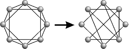
Figure 6: The construction of a small-word network according to Watts and Strogatz: A regular network has its edges rewired with probability $p$. For $p\approx 0$ the network is regular, with many triangles and large distances, for $p\approx 1$, the network becomes a random network, with small distances and few triangles.

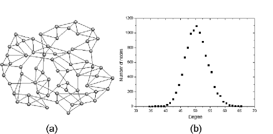
Figure 7: The small-world model of Watts and Strogatz: (a) an example of a network with $N=64$ vertices, $\kappa=2$, $p=0.1$, and (b) average degree distribution over $10$ WS networks with $10\,000$ vertices, $\kappa=25$ and $p=0.3$.

The degree distribution for small-world networks is similar to that of random networks, with a peak at $\langle k\rangle=2\kappa$ (see also Table 2).

3.3 Generalized Random Graphs

A common way to study real networks is to compare their characteristics with the values expected for similar random networks. As the degrees of the vertices are important features of the network, it is interesting to make the comparison with networks with the same degree distribution. Models to generate networks with a given degree distribution, while being random in other aspects, have been proposed.

Bender and Canfield [48] first proposed a model to generate random graphs with a pre-defined degree distribution called configuration model. Later, Molloy and Reed [49, 50] proposed a different method that produces multigraphs (i.e. loops and multiple edges between the same pair of vertices are allowed).

The common method used to generate this kind of random graph involves selecting a degree sequence specified by a set $\{k_{i}\}$ of degrees of the vertices drawn from the desired distribution $P(k)$. Afterwards, to each vertex $i$ is associated a number $k_{i}$ of “stubs” or “spokes” (ends of edges emerging from a vertex) according to the desired degree sequence. Next, pairs of such stubs are selected uniformly and joined together to form an edge. When all stubs have been used up, a random graph that is a member of the ensemble of graphs with that degree sequence is obtained [51, 52, 53].

Another possibility, the rewiring method, is to start with a network (possibly a real network under study) that already has the desired degree distribution, and then iteratively chose two edges and interchange the corresponding attached vertices [54]. This rewiring procedure is used in some results presented in Section 16.2.

Due to its importance and amenability to analytical treatment, many works deal with this model, including the papers of Newman [23], Aiello et al. [55], Chung and Lu [56] and Cohen and Havlin [57].

3.4 Scale-free Networks of Barabási and Albert

After Watts and Strogatz’s model, Barabási and Albert [9] showed that the degree distribution of many real systems is characterized by an uneven distribution. Instead of the vertices of these networks having a random pattern of connections with a characteristic degree, as with the ER and WS models (see Figure 5(a)), some vertices are highly connected while others have few connections, with the absence of a characteristic degree. More specifically, the degree distribution has been found to follow a power law for large $k$,

$$P(k)\sim k^{-\gamma}$$ (10)

(see Figure 8(b)). These networks are called scale-free networks.

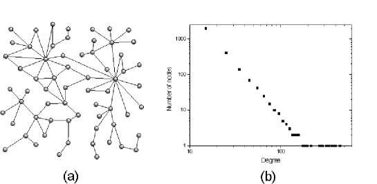
Figure 8: The scale-free network of Barabási and Albert. (a) an example of a scale-free network and (b) average degree distribution over $10$ Barabási-Albert networks formed by $10,000$ vertices using $m=5$. The degree distribution follows a power law, in contrast to that presented in Figure 5.

A characteristic of this kind of network is the existence of hubs, i.e. vertices that are linked to a significant fraction of the total number of edges of the network.

The Barabási-Albert (BA) network model is based on two basic rules: growth and preferential attachment. The network is generated starting with a set of $m_{0}$ vertices; afterwards, at each step of the construction the network grows with the addition of new vertices. For each new vertex, $m$ new edges are inserted between the new vertex and some previous vertex. The vertices which receive the new edges are chosen following a linear preferential attachment rule, i.e. the probability of the new vertex $i$ to connect with an existing vertex $j$ is proportional to the degree of $j$,

$$\mathcal{P}(i\rightarrow j)=\frac{k_{j}}{\sum_{u}k_{u}}.$$ (11)

Thus, the most connected vertices have greater probability to receive new vertices. This is known as “the rich get richer” paradigm.

Figure 8(a) shows an example of a Barabási-Albert network.

Table 2: Analytical result of some basic measurements for the Erdős-Rényi,Watts-Strogatz and Barabási-Albert network models.

Measurement	Erdős-Rényi	Watts-Strogatz	Barabási-Albert
Degree
distribution	$P(k)=\frac{e^{-\langle k\rangle}\langle k\rangle^{k}}{k!}$	$P(k)=\sum_{i=1}^{min(k-\kappa,\kappa)}\left(\begin{array}[]{c}\kappa\\ i\\ \end{array}\right)(1-p)^{i}p^{\kappa-i}\frac{(p\kappa)^{k-\kappa-i}}{(k-\kappa-i)!}e^{-p\kappa}$	$P(k)\sim k^{-3}$
Average
vertex degree	$\langle k\rangle=p(N-1)$	$\langle k\rangle=2\kappa^{\star}$	$\langle k\rangle=2m$
Clustering
coefficient	$C=p$	$C(p)\sim\frac{3(\kappa-1)}{2(2\kappa-1)}(1-p)^{3}$	$C\sim N^{-0.75}$
Average
path length	$\ell\sim\frac{\ln N}{\ln\langle k\rangle}$	$\ell(N,p)\sim p^{\tau}f(Np^{\tau})^{\ast}$	$\ell\sim\frac{\log N}{\log(\log N)}$

$\star$ In WS networks, the value $\kappa$ represents the number of neighbors of each vertex in the initial regular network (in Figure 6, $\kappa=4$).
$\ast$ The function $f(u)=$ constant if $u\ll 1$ or $f(u)=\ln(u)/u$ if $u\gg 1$.

3.5 Networks with Community Structure

Some real networks, such as social and biological networks, present modular structure [10]. These networks are formed by sets or communities of vertices such that most connections are found between vertices inside the same community, while connections between vertices of different communities are less common. A model to generate networks with this property was proposed by Girvan and Newman [10]. This model is a kind of random graph constructed with different probabilities. Initially, a set of $N$ vertices is classified into $c$ communities. At each following step, two vertices are selected and linked with probability $p_{\mathrm{in}}$, if they are in the same community, or $p_{\mathrm{out}}$, if they are in different communities. The values of $p_{\mathrm{in}}$ and $p_{\mathrm{out}}$ should be chosen so as to generate networks with the desired sharpness in the distinction of the communities. When $p_{\mathrm{out}}\ll p_{\mathrm{in}}$, the communities can be easily identified. On the other hand, when $p_{\mathrm{out}}\approx p_{\mathrm{in}}$, the communities become blurred.

Figure 9(a) presents a network generated by using the procedure above.

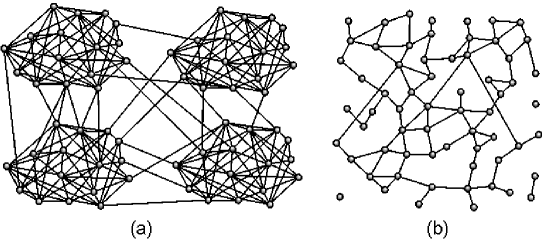
Figure 9: (a) An example of a random network with community structure formed by $64$ vertices divides in $4$ communities. (b) An example of geographical network formed by $64$ vertices.

3.6 Geographical Models

Complex networks are generally considered as lying in an abstract space, where the position of vertices has no particular meaning. In the case of several kinds of networks, such as protein-protein interaction networks or networks of movie actors, this consideration is reasonable. However, there are many networks where the position of vertices is particularly important as it influences the network evolution. This is the case of highway networks or the Internet, for example, where the position of cities and routers can be localized in a map and the edges between correspond to real physical entities, such as roads and optical fibers [58]. This kind of networks is called geographical or spatial networks. Other important examples of geographical networks are power grids [59, 60], airport networks [61, 62, 63], subway [64] and neural networks [65].

In geographical networks, the existence of a direct connection between vertices can depend on a lot of constraints such as the distance between them, geographical accidents, available resources to construct the network, territorial limitation and so on. The models considered to represent these networks should consider these constraints.

A simple way to generate geographical networks, used in the results described in Sections 16, 17, and 18, is to distribute $N$ vertices at random in a two-dimensional space $\Omega$ and link them with a given probability which decays with the distance, for instance

$$\mathcal{P}(i\rightarrow j)\sim e^{-\lambda s_{ij}}$$ (12)

where $s_{ij}$ is the geographical distance of the vertices and $\lambda$ fixes the length scale of the edges. This model generates a Poisson degree distribution as observed for random graphs and can be used to model road networks (see Figure 9(b)). Alternatively, the network development might start with few nodes while new nodes and connections are added at each subsequent time step (spatial growth). Such a model is able to generate a wide range of network topologies including small-world and linear scale-free networks  [66].

4 Measurements Related with Distance

For undirected, unweighted graphs, the number of edges in a path connecting vertices $i$ and $j$ is called the length of the path. A geodesic path (or shortest path), between vertices $i$ and $j$, is one of the paths connecting these vertices with minimum length (many geodesic paths may exist between two vertices); the length of the geodesic paths is the geodesic distance $d_{ij}$ between vertices $i$ and $j$. If the graph is weighted, the same definition can be used, but generally one is interested in taking into account the edge weights. Two main possibilities include: first, the edge weights may be proportionally related to some physical distance, for example if the vertices correspond to cities and the weights to distances between these cities through given highways. In this case, one can compute the distance along a path as the sum of the weights of the edges in the path. Second, the edge weights may reflect the strength of connection between the vertices, for example if the vertices are Internet routers and the weights are the bandwidth of the edges, the distance corresponding to each edge can be taken as the reciprocal of the edge weight, and the path length is the sum of the reciprocal of the weight of the edges along the path. If there are no paths from vertex $i$ to vertex $j$, then $d_{ij}=\infty.$ For digraphs, the same definitions can be used, but in general $d_{ij}\neq d_{ji}$, as the paths from vertex $i$ to vertex $j$ are different from the paths from $j$ to $i$.

Distance is an important characteristic that depends on the overall network structure. The following describes some measurements based on vertex distance.

4.1 Average Distance

We can define a network measurement by computing the mean value of $d_{ij}$, known as average geodesic distance:

$$\ell=\frac{1}{N(N-1)}\sum_{i\neq j}d_{ij}.$$ (13)

A problem with this definition is that it diverges if there are unconnected vertices in the network. To circumvent this problem, only connected pairs of vertices are included in the sum. This avoids the divergence, but introduces a distortion for networks with many unconnected pairs of vertices, which will show a small value of average distance, expected only for networks with a high number of connections. Latora and Marchiori [67] proposed a closely related measurement that they called global efficiency:

$$E=\frac{1}{N(N-1)}\sum_{i\neq j}\frac{1}{d_{ij}},$$ (14)

where the sum takes all pairs of vertices into account. This measurement quantifies the efficiency of the network in sending information between vertices, assuming that the efficiency for sending information between two vertices $i$ and $j$ is proportional to the reciprocal of their distance. The reciprocal of the global efficiency is the harmonic mean of the geodesic distances:

$$h=\frac{1}{E}.$$ (15)

As Eq. (15) does not present the divergence problem of Eq. (13), it is therefore a more appropriate measurement for graphs with more than one connected component.

The determination of shortest distances in a network is only possible with global information on the structure of the network. This information is not always available. When global information is unavailable, navigation in a network must happen using limited, local information and a specific algorithm. The effective distance between two vertices is thus generally larger than the shortest distance, and dependent on the algorithm used for navigation as well as network structure [68].

4.2 Vulnerability

In infrastructure networks (like WWW, the Internet, energy supply, etc), it is important to know which components (vertices or edges) are crucial to their best functioning. Intuitively, the critical vertices of a network are their hubs (vertices with higher degree), however there are situations in which they are not necessarily most vital for the performance of the system which the network underlies. For instance, all vertices of a network in the form of a binary tree have equal degree, therefore there is no hub, but disconnection of vertices closer to the root and the root itself have a greater impact than of those near the leaves. This suggests that networks have a hierarchical property, which means that the most crucial components are those in higher positions in the hierarchy.

A way to find critical components of a network is by looking for the most vulnerable vertices. If we associate the performance of a network with its global efficiency, Eq. (14), the vulnerability of a vertex can be defined as the drop in performance when the vertex and all its edges are removed from the network [69]

$$V_{i}=\frac{E-E_{i}}{E}$$ (16)

where $E$ is the global efficiency of the original network and $E_{i}$ is the global efficiency after the removal of the vertex $i$ and all its edges. As suggested by Gol’dshtein et al. [69], the ordered distribution of vertices with respect to their vulnerability $V_{i}$ is related to the network hierarchy, thus the most vulnerable (critical) vertex occupies the highest position in the network hierarchy.

A measurement of network vulnerability [70] is the maximum vulnerability for all of its vertices:

$$V=\max_{i}V_{i}.$$ (17)

5 Clustering and Cycles

A characteristic of the Erdős-Rényi model is that the local structure of the network near a vertex tends to be a tree. More precisely, the probability of loops involving a small number of vertices goes to $0$ in the large network size limit. This is in marked contrast with the profusion of short loops which appear in many real-world networks. Some measurements proposed to study the cyclic structure of networks and the tendency to form sets of tightly connected vertices are described in the following.

5.1 Clustering Coefficients

One way to characterize the presence of loops of order three is through the clustering coefficient.

Two different clustering coefficients are frequently used. The first, also known as transitivity [71], is based on the following definition for undirected unweighted networks:

$$C=\frac{3N_{\triangle}}{N_{3}},$$ (18)

where $N_{\triangle}$ is the number of triangles in the network and $N_{3}$ is the number of connected triples. The factor three accounts for the fact that each triangle can be seen as consisting of three different connected triples, one with each of the vertices as central vertex, and assures that $0\leq C\leq 1$. A triangle is a set of three vertices with edges between each pair of vertices; a connected triple is a set of three vertices where each vertex can be reached from each other (directly or indirectly), i.e. two vertices must be adjacent to another vertex (the central vertex). Therefore we have

$$N_{\triangle} = \sum_{k>j>i}a_{ij}a_{ik}a_{jk},$$ (19)

$$N_{3} = \sum_{k>j>i}(a_{ij}a_{ik}+a_{ji}a_{jk}+a_{ki}a_{kj}),$$ (20)

where the $a_{ij}$ are the elements of the adjacency matrix $A$ and the sum is taken over all triples of distinct vertices $i$, $j$, and $k$ only one time.

It is also possible to define the clustering coefficient of a given vertex $i$ [8] as:

$$C_{i}=\frac{N_{\triangle}(i)}{N_{3}(i)},$$ (21)

where $N_{\triangle}(i)$ is the number of triangles involving vertex $i$ and $N_{3}(i)$ is the number of connected triples having $i$ as the central vertex:

$$N_{\triangle}(i) = \sum_{k>j}a_{ij}a_{ik}a_{jk},$$ (22)

$$N_{3}(i) = \sum_{k>j}a_{ij}a_{ik},$$ (23)

If $k_{i}$ is the number of neighbors of vertex $i$, then $N_{3}(i)=k_{i}(k_{i}-1)/2$. $N_{\triangle}(i)$ counts the number of edges between neighbors of $i$. Representing the number of edges between neighbors of $i$ as $l_{i}$, Eq. (21) can be rewritten as:

$$C_{i}=\frac{2l_{i}}{k_{i}(k_{i}-1)}.$$ (24)

Using $C_{i}$, an alternative definition of the network clustering coefficient (different from that in Eq. (18)) is

$$\widetilde{C}=\frac{1}{N}\sum_{i}C_{i}.$$ (25)

The difference between the two definitions is that the average in Eq. (18) gives the same weight to each triangle in the network, while Eq. (25) gives the same weight to each vertex, resulting in different values because vertices of higher degree are possibly involved in a larger number of triangles than vertices of smaller degree.

For weighted graphs, Barthélemy [42] introduced the concept of weighted clustering coefficient of a vertex,

$$C^{w}_{i}=\frac{1}{s_{i}(k_{i}-1)}\sum_{(j,k)}\frac{w_{ij}+w_{ik}}{2}a_{ij}a_{ik}a_{jk},$$ (26)

where the normalizing factor $s_{i}(k_{i}-1)$ ($s_{i}$ is the strength of the vertex, see Section 2) assures that $0\leq C^{w}_{i}\leq 1$. From this equation, a possible definition of clustering coefficient for weighted networks is

$$C^{w}=\frac{1}{N}\sum_{i}C^{w}_{i}.$$ (27)

Another definition for clustering in weighted networks [72] is based on the intensity of the triangle subgraphs, (see Section 12.2),

$$\widetilde{C}_{i}^{w}=\frac{2}{k_{i}(k_{i}-1)}\sum_{(j,k)}(\hat{w}_{ij}\hat{w}_{jk}\hat{w}_{ki})^{1/3},$$ (28)

where $\hat{w}_{ij}=w_{ij}/\max_{ij}w_{ij}$.

Given the clustering coefficients of the vertices, the clustering coefficient can be expressed as a function of the degree of the vertices:

$$C(k)=\frac{\sum_{i}C_{i}\delta_{k_{i}k}}{\sum_{i}\delta_{k_{i}k}},$$ (29)

where $\delta_{ij}$ is the Kronecker delta. For some networks, this function has the form $C(k)\sim k^{-\alpha}$. This behavior has been associated with a hierarchical structure of the network, with the exponent $\alpha$ being called its hierarchical exponent [73]. Soffer and Vázquez [74] found that this dependence of the clustering coefficient with $k$ is to some extent due to the degree correlations (Section 6) of the networks, with vertices of high degree connecting with vertices of low degree. They suggested a new definition of clustering coefficient without degree correlation bias:

$$\hat{C}_{i}=\frac{l_{i}}{\omega_{i}},$$ (30)

where $l_{i}$ is the number of edges between neighbors of $i$ and $\omega_{i}$ is the maximum number of edges possible between the neighbors of vertex $i$, considering their vertex degrees and the fact that they are necessarily connected with vertex $i$.

5.2 Cyclic Coefficient

Kim and Kim [75] defined a cyclic coefficient in order to measure how cyclic a network is. The local cyclic coefficient of a vertex $i$ is defined as the average of the inverse of the sizes of the smallest cycles formed by vertex $i$ and its neighbors,

$$\Theta_{i}=\frac{2}{k_{i}(k_{i}-1)}\sum_{(j,k)}{\frac{1}{S_{ijk}}a_{ij}a_{ik}},$$ (31)

where $S_{ijk}$ is the size of the smallest cycle which passes through vertices $i$, $j$ and $k$. Note that if vertices $j$ and $k$ are connected, the smallest cycle is a triangle and $S_{ijk}=3$. If there is no loop passing through $i$, $j$ and $k$, then these vertices are tree-like connected and $S_{ijk}=\infty$. The cyclic coefficient of a network is the average of the cyclic coefficient of all its vertices:

$$\Theta=\frac{1}{N}\sum_{i}\Theta_{i}.$$ (32)

5.3 Rich-Club Coefficient

In science, influential researchers of some areas tend to form collaborative groups and publish papers together [76]. This tendency is observed in other real networks and reflect the tendency of hubs to be well connected with each other. This phenomenon, known as rich-club, can be measured by the rich-club coefficient, introduced by Zhou and Mondragon [77]. The rich-club of degree $k$ of a network $G$ is the set of vertices with degree greater than $k$, $\mathcal{R}(k)=\{v\in\mathcal{N}(G)|k_{v}>k\}.$ The rich-club coefficient of degree $k$ is given by

$$\phi(k)=\frac{1}{|\mathcal{R}(k)|(|\mathcal{R}(k)|-1)}\sum_{i,j\in\mathcal{R}(k)}a_{ij}$$ (33)

(the sum corresponds to two times the number of edges between vertices in the club). This measurement is similar to that defined before for the clustering coefficient (see Eq. (24)), giving the fraction of existing connections among vertices with degree higher than $k$.

Colizza et al. [76] derived an analytical expression of the rich-club coefficient, valid for uncorrelated networks,

$$\phi_{\mathrm{unc}}(k)\sim\frac{k^{2}}{\langle k\rangle N}.$$ (34)

The definition of the weighted rich-club coefficient for weighted networks is straightforward. If $\mathcal{R}^{w}(s)$ is the set of vertices with strength greater than $s$, $\mathcal{R}^{w}(s)=\{v\in G|s_{v}>s\},$

$$\phi^{w}(s)=\frac{\sum_{i,j\in\mathcal{R}^{w}(s)}w_{ij}}{\sum_{i\in\mathcal{R}^{w}(s)}s_{i}}$$ (35)

(the sum in the numerator give two times the weight of the edges between elements of the rich-club, the sum in the denominator gives the total strength of the vertices in the club).

6 Degree Distribution and Correlations

The degree is an important characteristic of a vertex [78]. Based on the degree of the vertices, it is possible to derive many measurements for the network. One of the simplest is the maximum degree:

$$k_{\mathrm{max}}=\max_{i}k_{i}.$$ (36)

Additional information is provided by the degree distribution, $P(k)$, which expresses the fraction of vertices in a network with degree $k$. An important property of many real world networks is their power law degree distribution [9]. For directed networks there are an out-degree distribution $P^{\mathrm{out}}(k^{\mathrm{out}})$, an in-degree distribution $P^{\mathrm{in}}(k^{\mathrm{in}})$, and the joint in-degree and out-degree distribution $P^{\mathrm{io}}(k^{\mathrm{in}},k^{\mathrm{out}})$. The latter distribution gives the probability of finding a vertex with in-degree $k\mathrm{in}$ and out-degree $k_{\mathrm{out}}$. Similar definitions considering the strength of the vertices can be used for weighted networks. An objective quantification of the level to which a log-log distribution of points approach a power law can be provided by the respective Pearson coefficient, which is henceforth called straightness and abbreviated as $\mathit{st}$.

It is often interesting to check for correlations between the degrees of different vertices, which have been found to play an important role in many structural and dynamical network properties [79]. The most natural approach is to consider the correlations between two vertices connected by an edge. This correlation can be expressed by the joint degree distribution $P(k,k^{\prime})$, i.e. as the probability that an arbitrary edge connects a vertex of degree $k$ to a vertex of degree $k^{\prime}$. Another way to express the dependence between vertex degrees is in terms of the conditional probability that an arbitrary neighbor of a vertex of degree $k$ has degree $k^{\prime}$ [80, 81],

$$P(k^{\prime}|k)=\frac{\langle k\rangle P(k,k^{\prime})}{kP(k)}.$$ (37)

Notice that $\sum_{k^{\prime}}P(k^{\prime}|k)=1$. For undirected networks, $P(k,k^{\prime})=P(k^{\prime},k)$ and $k^{\prime}P(k|k^{\prime})P(k^{\prime})=kP(k^{\prime}|k)P(k)$. For directed networks, $k$ is the degree at the tail of the edge, $k^{\prime}$ is the degree at the head, both $k$ and $k^{\prime}$ may be in-, out-, or total degrees, and in general $P(k,k^{\prime})\neq P(k,k^{\prime})$. For weighted networks the strength $s$ can be used instead of $k$.

$P(k,k^{\prime})$ and $P(k|k^{\prime})$ characterize formally the vertex degree correlations, but they are difficult to evaluate experimentally, especially for fat-tailed distributions, as a consequence of the finite network size and the resulting small sample of vertices with high degree. This problem can be addressed by computing the average degree of the nearest neighbors of vertices with a given degree $k$ [82], which is given by

$$k_{\mathrm{nn}}(k)=\sum_{k^{\prime}}k^{\prime}P(k^{\prime}|k).$$ (38)

If there are no correlations, $k_{\mathrm{nn}}(k)$ is independent of $k$, $k_{\mathrm{nn}}(k)=\langle k^{2}\rangle/\langle k\rangle$. When $k_{\mathrm{nn}}(k)$ is an increasing function of $k$, vertices of high degree tend to connect with vertices of high degree, and the network is classified as assortative, whereas whenever $k_{\mathrm{nn}}(k)$ is a decreasing function of $k$, vertices of high degree tend to connect with vertices of low degree, and the network is called disassortative [83].

Another way to determine the degree correlation is by considering the Pearson correlation coefficient of the degrees at both ends of the edges [83]:

$$r=\frac{\frac{1}{M}\sum_{j>i}k_{i}k_{j}a_{ij}-\left[\frac{1}{M}\sum_{j>i}\frac{1}{2}(k_{i}+k_{j})a_{ij}\right]^{2}}{\frac{1}{M}\sum_{j>i}\frac{1}{2}(k_{i}^{2}+k_{j}^{2})a_{ij}-\left[\frac{1}{M}\sum_{j>i}\frac{1}{2}(k_{i}+k_{j})a_{ij}\right]^{2}},$$ (39)

where $M$ is the total number of edges. If $r>0$ the network is assortative; if $r<0$, the network is disassortative; for $r=0$ there are no correlation between vertex degrees.

Degree correlations can be used to characterize networks and to validate the ability of network models to represent real network topologies. Newman [83] computed the Pearson correlation coefficient for some real and model networks and discovered that, although the models reproduce specific topological features such as the power law degree distribution or the small-world property, most of them (e.g., the Erdő-Rényi and Barabási-Albert models) fail to reproduce the assortative mixing ($r=0$ for the Erdő-Rényi and Barabási-Albert models). Further, it was found that the assortativity depends on the type of network. While social networks tend to be assortative, biological and technological networks are often disassortative. The latter property is undesirable for practical purposes, because assortative networks are known to be resilient to simple target attack, at the least. So, for instance, in disease propagation, social networks would ideally be vulnerable (i.e. the network is dismantled into connected components, isolating the focus of disease) and technological and biological networks should be resilient against attacks. The degree correlations are related to the network evolution process and, therefore, should be taken into account in the development of new models as done, for instance, in the papers by Catanzaro et al. [84] on social networks, Park and Newman [85] on the Internet, and Berg et al. [86] on protein interaction networks. Degree correlations also have strong influence on dynamical processes like instability [87], synchronization [88, 89] and spreading [80, 90, 91]. For additional discussions about dynamical process as in networks see Ref. [24].

7 Networks with Different Vertex Types

Some networks include vertices of different types. For example, in a sociological network where the vertices are people and the edges are a social relation between two persons (e.g., friendship), one may be interested in answering questions like: how probable is a friendship relation between two persons of different economic classes? In this case, it is interesting to consider that the vertices are not homogeneous, having different types. In the following, measurements associated with such kind of networks are discussed.

7.1 Assortativity

For networks with different types of vertices, a type mixing matrix $E$ can be defined, with elements $e_{st}$ such that $e_{st}$ is the number of edges connecting vertices of type $s$ to vertices of type $t$ (or the total strength of the edges connecting the two vertices of the given types, for weighted networks). It can be normalized as

$$\hat{E}=\frac{E}{\|E\|},$$ (40)

where $\|X\|$ (cardinality) represents the sum of all elements of matrix $X$.

The probability of a vertex of type $s$ having a neighbor of type $t$ therefore is

$$P^{\mathrm{(type)}}(t|s)=\frac{\hat{e}_{st}}{\sum_{u}\hat{e}_{su}}.$$ (41)

Note that $\sum_{t}P^{\mathrm{(type)}}(t|s)=1.$

$P^{\mathrm{(type)}}(s,t)$ and $\hat{E}$ can be used to quantify the tendency in the network of vertices of some type to connect to vertices of the same type, called assortativity. We can define an assortativity coefficient [92, 23] as:

$$\widetilde{\mathbb{Q}}=\frac{\sum_{s}P^{\mathrm{(type)}}(s|s)-1}{N_{T}-1},$$ (42)

where $N_{T}$ is the number of different vertex types in the network. It can be seen that $0\leq\tilde{\mathbb{Q}}\leq 1$, where $\tilde{\mathbb{Q}}=1$ for a perfectly assortative network (only edges between vertices of the same type) and $\tilde{\mathbb{Q}}=0$ for random mixing. But each vertex type has the same weight in $\tilde{\mathbb{Q}}$, regardless of the number of vertices of that type. An alternative definition that avoids this problem [93] is:

$$\mathbb{Q}=\frac{\mathrm{Tr}\,\hat{E}-\|\hat{E}^{2}\|}{1-\|\hat{E}^{2}\|}.$$ (43)

It is interesting to associate the vertex type to its degree. The Pearson correlation coefficient of vertex degrees, Eq. (39), can be considered as an assortativity coefficient for this case.

7.2 Bipartivity Degree

A special case of disassortativity is that of bipartite networks. A network is called bipartite if its vertices can be separated into two sets such that edges exist only between vertices of different sets. It is a known fact that a network is bipartite if and only if it has no loops of odd length (e.g. [94]). Although some networks are bipartite by construction, others, like a network of sexual contacts, are only approximately bipartite. A way to quantify how much a network is bipartite is therefore needed. A possible measurement is based on the number of edges between vertices of the same subset in the best possible division [94],

$$b=1-\frac{\sum_{ij}a_{ij}\delta_{\vartheta(i),\vartheta(j)}}{\sum_{ij}a_{ij}},$$ (44)

where $\vartheta(i)$ maps a vertex $i$ to its type and $\delta$ is the Kronecker delta. The smallest value of $b$ for all possible divisions is the bipartivity of the network. The problem with this measurement is that its computation is NP-complete, due to the necessity of evaluating $b$ for the best possible division. A measurement that approximates $b$ but is computationally easier was proposed in [94], based on a process of marking the minimum possible number of edges as responsible for the creation of loops of odd length.

Another approach is based on the subgraph centrality [95] (Section 12.3). The subgraph centrality of the network, Eq. (84), is divided in a part due to even closed walks and a part due to odd closed walks (a closed walk is a walk, possibly with repetition of vertices, ending on the starting vertex). As odd closed walks are not possible in bipartite networks, the fraction of the subgraph centrality of the network due to even closed walks can be used as the bipartivity degree [95]:

$$\beta=\frac{\mathit{SC}_{\mathrm{even}}}{\mathit{SC}}=\frac{\sum_{j=1}^{N}\cosh\lambda_{j}}{\sum_{j=1}^{N}e^{\lambda_{j}}},$$ (45)

where $\mathit{SC}$ is the subgraph centrality of the network (Section 12.3), $\mathit{SC}_{\mathrm{even}}$ is the subgraph centrality due to the even closed walks and the $\lambda_{j}$ are the eigenvalues of the adjacency matrix of the network.

8 Entropy

Entropy is a key concept in thermodynamics, statistical mechanics [96] and information theory [97]. It has important physical implications related to the amount of “disorder” and information in a system [98]. In information theory, entropy describes how much randomness is present in a signal or random event [99]. This concept can be usefully applied to complex networks.

8.1 Entropy of the Degree Distribution

The entropy of the degree distribution provides an average measurement of the heterogeneity of the network, which can be defined as

$$H=-\sum_{k}P(k)\log P(k).$$ (46)

The maximum value of entropy is obtained for a uniform degree distribution and the minimum value $H_{\mathrm{min}}=0$ is achieved whenever all vertices have the same degree [100]. Network entropy has been related to the robustness of networks, i.e. their resilience to attacks [100], and the contribution of vertices to the network entropy is correlated with lethality in protein interactions networks [101].

Solé and Valverde [102] suggested the use of the remaining degree distribution to compute the entropy. The remaining degree of a vertex at one end of an edge is the number of edges connected to that vertex not counting the original edge. The remaining degree distribution can be computed as

$$q(k)=\frac{(k+1)P(k+1)}{\langle k\rangle}.$$ (47)

The entropy of the remaining degree is given by

$$H^{*}=-\sum_{k}q(k)\log q(k).$$ (48)

8.2 Search Information, Target Entropy and Road Entropy

The structure of a complex network is related to its reliability and information propagation speed. The difficulty while searching information in the network can be quantified through the information entropy of the network [103, 104]. Rosvall et al. [105] introduced measurements to quantify the information associated to locating a specific target in a network. Let $p(i,b)$ be a shortest path starting at vertex $i$ and ending at vertex $b$. The probability to follow this path in a random walk is

$$\mathcal{P}[p(i,b)]=\frac{1}{k_{i}}\prod_{j\in p(i,b)}\frac{1}{k_{j}-1},$$ (49)

where $k_{j}$ is the degree of vertex $j$ and the product includes all vertices $j$ in the path $p(i,b)$ with the exclusion of $i$ and $b$. The search information, corresponding to the total information needed to identify one of the shortest paths between $i$ and $b$, is given by

$$\mathcal{S}(i,b)=-\log_{2}\sum_{\{p(i,b)\}}\mathcal{P}[p(i,b)],$$ (50)

where the sum is taken over all shortest paths $p(i,b)$ from $i$ to $b$.

The average search information characterizes the ease or difficulty of navigation in a network and is given by [105]

$$\mathcal{S}=\frac{1}{N^{2}}\sum_{ij}\mathcal{S}(i,b).$$ (51)

This value depends on the structure of the network. As discussed by Rosvall et al. [105], city networks are more difficult to be navigated than their random counterparts.

In order to measure how difficult it is to locate vertices in the network starting from a given vertex $i$, the access information is used,

$$\mathcal{A}_{i}=\frac{1}{N}\sum_{b}\mathcal{S}(i,b),$$ (52)

which measures the average number of “questions” needed to locate another vertex starting from $i$. To quantify how difficult is to find the vertex $b$ starting from the other vertices in the network, the hide information is used,

$$\mathcal{H}_{b}=\frac{1}{N}\sum_{i}\mathcal{S}(i,b).$$ (53)

Note that the average value of $\mathcal{A}_{i}$ and $\mathcal{H}_{b}$ for a network is $\mathcal{S}$: $\sum_{i}\mathcal{A}_{i}=\sum_{b}\mathcal{H}_{b}=\mathcal{S}N$.

Considering the exchange of messages in the network, it is possible to define entropies in order to quantify the predictability of the message flow. Assuming that messages always flow through shortest paths and all pairs of vertices exchange the same number of messages at the same rate, the following entropies can be defined [103]:

$$\mathcal{T}_{i} = -\sum_{ij}a_{ji}c_{ij}\log_{2}c_{ij},$$ (54)

$$\mathcal{R}_{i} = -\sum_{ij}a_{ji}b_{ij}\log_{2}b_{ij},$$ (55)

where $a_{ji}$ is an element of the adjacency matrix, $c_{ij}$ is the fraction of messages targeted at vertex $i$ that comes through vertex $j$, and $b_{ij}$ is the fraction of messages that goes through vertex $i$ coming from vertex $j$. In addition, $\mathcal{T}_{i}$ is the target entropy of vertex $i$ and $\mathcal{R}_{i}$ is the road entropy of vertex $i$. Low values of these entropies mean that the vertex from where the next message originates (to vertex $i$ or passing through vertex $i$) can be easily predicted.

As a general measurement of the flows of messages, we can define target and road entropies for the network as averages among all vertices

$$\mathcal{T} = \frac{1}{N}\sum_{i}\mathcal{T}_{i},$$ (56)

$$\mathcal{R} = \frac{1}{N}\sum_{i}\mathcal{R}_{i}.$$ (57)

As shown in [103], these quantities are related to the organization of the network: a network with a low value of $\mathcal{T}$ has a star structure and a low value of $\mathcal{R}$ means that the network is composed by hubs connected in a string.

Further works related to searchability in networks have been reported by Trusina et al. [106], who defined a search information weighted by the traffic on the network, and Rosvall et al. [107] who studied networks with higher order organization like modular or hierarchical structure.

9 Centrality Measurements

In networks, the greater the number of paths in which a vertex or edge participates, the higher the importance of this vertex or edge for the network. Thus, assuming that the interactions follow the shortest paths between two vertices, it is possible to quantify the importance of a vertex or a edge in terms of its betweenness centrality [108] defined as:

$$B_{u}=\sum_{ij}\frac{\sigma(i,u,j)}{\sigma(i,j)},$$ (58)

where $\sigma(i,u,j)$ is the number of shortest paths between vertices $i$ and $j$ that pass through vertex or edge $u$, $\sigma(i,j)$ is the total number of shortest paths between $i$ and $j$, and the sum is over all pairs $i,j$ of distinct vertices.

When one takes into account the fact that the shortest paths might not be known and instead a search algorithm is used for navigation (see Section 4.1), the betweenness of a vertex or edge must be defined in terms of the probability of it being visited by the search algorithm. This generalization, which was introduced by Arenas et al. [109], subsumes the betweenness centrality based on random walks as proposed by Newman [110].

The central point dominance is defined as [108]

$$\mathit{CPD}=\frac{1}{N-1}\sum_{i}(B_{\mathrm{max}}-B_{i}),$$ (59)

where $B_{\mathrm{max}}$ is the largest value of betweenness centrality in the network. The central point dominance will be $0$ for a complete graph and $1$ for a star graph in which there is a central vertex included in all paths. Other centrality measurements can be found in the interesting survey by Koschützki et al. [111].

10 Spectral Measurements

The spectrum of a network corresponds to the set of eigenvalues $\lambda_{i}$ ($i=1,2,\ldots,N$) of its adjacency matrix $A$. The spectral density of the network is defined as [112, 113]:

$$\rho(\lambda)=\frac{1}{N}\sum_{i}\delta(\lambda-\lambda_{i}),$$ (60)

where $\delta(x)$ is the Dirac delta function and $\rho$ approaches a continuous function as $N\rightarrow\infty$; e.g., for Erdős-Rényi networks, if $p$ is constant as $N\rightarrow\infty$, $\rho(\lambda)$ converges to a semicircle [112]. Also, the eigenvalues can be used to compute the $l$th-moments,

$$M_{l}=\frac{1}{N}\sum_{i_{1},i_{2},\ldots,i_{l}}a_{i_{1}i_{2}}a_{i_{2}i_{3}}\cdots a_{i_{l}i_{1}}=\frac{1}{N}\sum_{i}(\lambda_{i})^{l}.$$ (61)

The eigenvalues and associated eigenvectors of a network are related to the diameter, the number of cycles and connectivity properties of the network [112, 113]. The quantity $D_{l}=NM_{l}$ is the number of paths returning to the same vertex in the graph passing through $l$ edges. Note that these paths can contain already visited vertices. Because in a tree-like graph a return walk is only possible going back through the already visited edges, the presence of odd moments is a sure sign of cycles in the graph; in particular, as a walk can go through three edges and return to its starting vertex only by following three different edges (if self-connections are not allowed), $D_{3}$ is related with the number of triangles in the network [113].

In addition, spectral analysis allows the identification whether a network is bipartite (if it does not contain any odd cycle [95], see section 7.2), characterizing models of real networks [114, 115], and visualizing networks [116]. In addition, spectral analysis of networks is important to determine communities and subgraphs, as discussed in the next section.

11 Community Identification and Measurements

Many real networks present an inhomogeneous connecting structure characterized by the presence of groups whose vertices are more densely interconnected one another than with the rest of the network. This modular structure has been found in many kinds of networks such as social networks [117, 118], metabolic networks [119] and in the worldwide flight transportation network [62]. Figure 10 presents a network with a well-defined community structure.

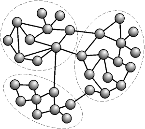
Figure 10: A network with community structure represented by the dashed lines. The communities are the groups of more intensely interconnected vertices.

Community identification in large networks is particularly useful because vertices belonging to the same community are more likely to share properties and dynamics. In addition, the number and characteristics of the existing communities provide subsidies for identifying the category of a network as well as understanding its dynamical evolution and organization. In the case of the World Wide Web, for instance, pages related to the same subject are typically organized into communities, so that the identification of these communities can help the task of seeking for information. Similarly, in the case of the Internet, information about communities formed by routers geographically close one another can be considered in order to improve the flow of data.

Despite the importance of the concept of community, there is no consensus about its definition. An intuitive definition was proposed by Radichi et al. [120] based on the comparison of the edge density among vertices. Communities are defined in a strong and a weak sense. In a strong sense, a subgraph is a community if all of its vertices have more connections between them than with the rest of the network. In a weak sense, on the other hand, a subgraph is a community if the sum of all vertex degrees inside the subgraph is larger than outside it. Though these definitions are intuitive, one of their consequences is that every union of communities is also a community. To overcome this limitation a hierarchy among the communities can be assumed a priori, as discussed by Reichardt and Bornholdt [121], who defined community in networks as the spin configuration that minimizes the energy of the spin glass by mapping the community identification problem onto finding the ground state of a infinite range Potts spin glass [122, 123].

Another fundamental related problem concerns how to best divide a network into its constituent communities. In real networks, no information is generally available about the number of existing communities. In order to address this problem, a measurement of the quality of a particular division of networks was proposed by Newman and Girvan [124], called modularity and typically represented by $Q$. If a particular network is split into $c$ communities, $Q$ can be calculated from the symmetric $c\times c$ mixing matrix $E$ whose elements along the main diagonal, $e_{ii}$, give the fraction of connections between vertices in the same community $i$ while the other elements, $e_{ij}$ ($i\neq j)$ identify the fraction of connections between vertices in the different communities $i$ and $j$. This is similar to the definition used to compute assortativity, Section 7. The calculation of $Q$ can then be performed as follows:

$$Q=\sum_{i}[e_{ii}-(\sum_{j}e_{ij})^{2}]=\mathrm{Tr}E-||E^{2}||,$$ (62)

The situation $Q=1$ identifies networks formed by disconnected modules. This quantity has been used in many community-finding algorithms, as briefly reviewed in the following.

Though there are many ways to defined modularity, a generally accepted definition of a module does not exist [125]. The definitions described above estimate the modularity in terms of a given partitioning. Ziv et al. [126] proposed the modularity to be defined in terms of information entropy (see Section 8). This algorithm, which has been called the Network Information Bottleneck, tends to allow performance better than the algorithm based on betweenness centrality of Girvan and Newman.

It should be noted that this review of community finding methods focus the subject of how specific network measurements have been adopted to identify the communities. Since we do not attempt to provide a comprehensive study of this important subject, the interested reader should refer to recent papers by Newman [127] and Danon et al. [128] for further information and a more complete review of community finding methods. The following discussion has been organized into subsections according to the nature of the adopted methodology.

11.1 Spectral Methods

Spectral methods are based on the analysis of the eigenvectors of matrices derived from the networks [129]. These methods have been discussed in a recent survey by Newman [130]. The quantity measured corresponds to the eigenvalues of matrices associated with the adjacency matrix. These matrices can be the Laplacian matrix (also known as Kirchhoff matrix),

$$L=D-A,$$ (63)

or the Normal matrix,

$$\tilde{A}=D^{-1}A,$$ (64)

where $D$ is the diagonal matrix of vertex degrees with elements $d_{ii}=\sum_{j}a_{ij},$ $d_{ij}=0$ for $i\neq j$.

A particular method, called spectral bisection [131, 132, 130], is based on the diagonalization of the Laplacian matrix. If the network is separated into $c$ disconnected components, $L$ will be block diagonal and have $c$ degenerated eigenvectors, all corresponding to eigenvalue $0$. However, if the separation is not clear, the diagonalization of $L$ will produce one eigenvector with eigenvalues $0$ and $c-1$ eigenvalues slightly different from $0$. The spectral bisection considers the case when $c=2$ and the division of the network is obtained assigning positive components of the eigenvector associated with the second eigenvalue (the positive eigenvalue most close to $0$) to one community and the negative ones to another community. Particularly, the second eigenvalue, called algebraic connectivity, is a measurement of how good the division is, with small values corresponding to better divisions. Although spectral bisection is easy to implement, it tends to be a poor approach for detecting communities in real networks [130]. There are many alternative methods based on spectral analysis [133], to be found in [127, 128].

Recently, Newman [134] proposed a method which reformulates the modularity concept in terms of the eigenvectors of a new characteristic matrix for the network, called modularity matrix. For each subgraph $g$, its modularity matrix $B^{(g)}$ has elements

$$b_{ij}^{(g)}=a_{ij}-\frac{k_{i}k_{j}}{2M}-\delta_{ij}\sum_{u\in\mathcal{N}(g)}\left[a_{iu}-\frac{k_{i}k_{u}}{2M}\right],$$ (65)

for vertices $i$ and $j$ in $g$. Thus, in order to split the network in communities, first the modularity matrix is constructed and its most positive eigenvalue and corresponding eigenvector are determined. According to the signs of the elements of this vector, the network is divided into two parts (vertices with positive elements are assigned to a community and vertices with negative elements to another). Next, the process is repeated recursively to each community until a split which makes zero or a negative contribution to the total modularity is reached. Following this idea, Newman proposed a new definition of communities as indivisible subgraphs, i.e. subgraphs whose division would increase the modularity. Currently, this method is believed to be the most precise, as it is able to find a division with the highest value of modularity for many networks [134].

11.2 Divisive Methods

In a divisive method, the underlying idea is to find the edges which connect different communities and remove them in a iterative form, breaking the network into disconnected groups of vertices. The computation of modularity can be used afterwards to determine the best division of the network. Next we give a brief description of the most known divisive methods according to the adopted measurement used to choose the vertex to remove.

11.2.1 Betweenness Centrality

The most popular divisive method is the Girvan-Newman algorithm [10]. Because different communities are connected by a small number of edges, this method considers that bottlenecks are formed at the edges which connect communities, through which all shortest paths should pass. In order to measure this traffic-related property in networks, the algorithm uses the concept of edge betweenness [10], see Section 9. Edges with high betweenness are progressively removed. After removing each edge, the betweenness of each remaining edge must be calculated again.

Although this algorithm represents a powerful alternative to determine communities (as shown in Figure 11), it has some disadvantages. The main one is its high computational cost. As discussed by Girvan and Newman [10], the entire algorithm runs in worst-case time $O(M^{2}N)$ on networks with $M$ edges and $N$ vertices. In order to overcome this limitation, some improvements in the algorithm were proposed including the Tyler’s algorithm [135], which introduced a stochastic element to the method, restricting the calculation of the betweenness only to a partial set of edges and using statistics to estimate the real betweenness.

11.2.2 Edge Clustering Coefficient

A different approach was proposed by Radicchi et al. [120] (see also [136]), which is based on counting short loops of order $l$ (triangles for $l=3$) in networks. The algorithm is similar to Girvan and Newman’s method, but instead of the betweenness centrality, it computes the edge clustering coefficient. This measurement is based on the fact that edges which connect communities tend to exhibit a small value for this coefficient. The clustering coefficient of edge $(i,j)$ is calculated as

$$C_{ij}=\frac{Z_{ij}+1}{\min(k_{i}-1,k_{j}-1)}$$ (66)

where $Z_{ij}$ is the number of triangles to which $(i,j)$ belongs. This method can be generalized to more complex loops, e.g., squares. Though this method is simple and fast ($O(M^{4}/N^{2})$), it fails whenever the network has a small average clustering coefficient, because the value of $C_{ij}$ will be small for all edges. This suggests that the method will work well only when applied to networks with a high average clustering coefficient, such as social networks [128].

11.3 Agglomerative Methods

Some networks are characterized by the fact that the vertices belonging to each community present similar features. So, it is in principle possible to obtain the communities by considering such similarities between vertices. In contrast to divisive methods, agglomerative approaches start with all vertices disconnected and then apply some similarity criterion to progressively join them and obtain the communities. It is interesting to note that this type of method presents a direct relationship with pattern recognition and clustering theory and algorithms (e.g., [137, 138, 139, 39]), which have been traditionally used in order to group individuals represented by a vector of features into meaningful clusters.

11.3.1 Similarity Measurements

One important family of agglomerative methods is known as hierarchical clustering [137, 138, 39, 13], which starts with $N$ vertices and no edges. Edges are added progressively to the network in decreasing order of similarity, starting with the pair with strongest similarity [140, 127]. To evaluate the similarity associated with edge $(i,j)$, a possibility is to use the so called Euclidian distance, given by

$$\sqrt{\sum_{k\neq i,j}(a_{ik}-a_{jk})^{2}},$$ (67)

or the Pearson correlation between vertices as represented in the adjacency matrix, defined as

$$\frac{\frac{1}{N}\sum_{k}(a_{ik}-\mu_{i})(a_{jk}-\mu_{j})}{\sigma_{i}\sigma_{j}},$$ (68)

where $\mu_{i}=\frac{1}{N}\sum_{j}a_{ij}$ and $\sigma_{i}^{2}=\frac{1}{N-1}\sum_{j}(a_{ij}-\mu_{i})^{2}.$

Although this method is fast, the obtained division of the network is not generally satisfactory for real networks, as discussed in [127].

11.4 Maximization of the Modularity

Newman [124, 141] proposed a method based on joining communities in such a way as to maximize the modularity. In this method, two communities $i$ and $j$ are joined according to a measurement of affinity, given by the change of the modularity $Q$ of the network (Eq. 62) when the communities are joined

$$\Delta Q_{ij}=2\left(e_{ij}-\frac{\sum_{j}e_{ij}\sum_{i}e_{ij}}{2M}\right).$$ (69)

Thus, starting with each vertex disconnected and considering each of them as a community, we repeatedly join communities together in pairs, choosing at each step the joining that results in the greatest increase (or smallest decrease) in the modularity $Q$. This process can be repeated until the whole network is contained in one community. Currently, as discussed by Danon et al. [128], the Newman’s method is believed to be the fastest one, running in $O(N\log^{2}N)$. Also, this method is more precise than the traditional method based on betweenness centrality [124]. However, as discussed by Danon et al. [142], the fast Newman’s method has a limitation when the size of communities is not homogeneous, as a newly joined community $i$ has the new values of $e_{ij}$ in Eq. 69 increased, and tends to be chosen for new joining. In real networks the distribution of sizes of communities tends to follow a power law. So, this approach fails in many real networks. In order to overcome this limitation, it was proposed [142] to normalize the value of $\Delta Q$ by the number of edges in community $i$,

$$\Delta\widehat{Q}_{ij}=\frac{\Delta Q_{ij}}{\sum_{j}e_{ij}}=\frac{2}{\sum_{j}e_{ij}}\left(e_{ij}-\frac{\sum_{j}e_{ij}\sum_{i}e_{ij}}{2M}\right).$$ (70)

This alteration on the local modularity makes the method more precise while not affecting its execution time.

11.4.1 Extremal Optimization

The extremal optimization method proposed by Duch and Arenas [143] is a heuristic search for optimizing the value of the modularity $Q$. The local modularity represents the contribution of individual vertex $i$ to the modularity $Q$. If $c_{i}$ is the community of vertex $i$, the local modularity is given by

$$q_{i}=\sum_{j}a_{ij}\delta_{c_{i},c_{j}}-k_{i}\sum_{c_{k}}e_{c_{i}c_{k}}$$ (71)

where $e_{ij}$ are the elements of the community mixing matrix (page 11) and $\delta$ is the Kronecker delta. In order to keep the value of this contribution in the interval $[-1,1]$ and independent of vertex degree, it should be normalized by the degree of the vertex, i.e. $\hat{q}_{i}=q_{i}/k_{i}$. The value of $\hat{q}_{i}$ is used as the fitness for the extremal optimization algorithm. A heuristic search is performed to obtain the maximum value of the modularity. Initially, the network is split into two random partitions with the same number of vertices. After each step, the system self-organizes by moving the vertex with lowest fitness from one partition to another. The process stops when the maximum value of $Q$ is reached.

Although this method is not particularly fast, scaling as $O(N^{2}\log N)$, it can achieve high modularity values [143]. By comparing the precision of some methods as presented in Figure 11, we can see that the extremal optimization method is more precise than the methods based on removing edges with highest betweenness centrality value. Moreover, it is clear that the computation of betweenness centrality by counting the number of shortest paths passing through each edge is more precise than calculating this coefficient by random walks [124].

Figure 11: Comparison of precision between the methods developed by Girvan and Newman [10] (based on removing edges with highest betweenness centrality value), the same method based on random walks [144], and the method developed by Duch and Arenas, based on extremal optimization [143]. Each point in this graph is an average of 100 realizations of networks with 128 vertices organized into 4 communities.

11.5 Local Methods

More recently, some methods have been developed to detect the local community of a vertex based only on local information about the network topology. One such method was proposed by Bagrow and Bolt [145], which is based on the change of the hierarchical degree between two consecutive distances (see Section 13). Starting from a vertex $v_{0}$, the vertices of successive hierarchical rings are added to the community, as long as the relation between the successive hierarchical degrees is greater than a specified threshold $\alpha$

$$\frac{k_{d}(v_{0})}{k_{d-1}(v_{0})}>\alpha.$$ (72)

When the expansion reaches a distance $d$ for which the above condition fails, the community stops growing.

Despite its favorable speed, this approach has an important limitation: the division is precise only when $v_{0}$ is equidistant from all parts of its enclosing community’s boundary [146]. In order to overcome this drawback, it has been suggested [145] that the algorithm be executed $N$ times starting from each vertex and then achieve a consensus about the detected communities. However, this approach increases the execution time of the algorithm.

Another local method was proposed by Clauset [146] which is based on computing the local modularity. The idea is that of a step-by-step growth of the community together with the exploration of the network. The community $\mathcal{C}$ starts with only the original vertex $v_{0}$. When a vertex is explored, a list of its neighbors is known. The set $\mathcal{U}$ is a list of all vertices that are not in $\mathcal{C}$ but are adjacent to some of its vertices; the set $\mathcal{B}$ (the boundary of $\mathcal{C}$) is the subset of vertices in $\mathcal{C}$ that are adjacent of at least one vertex in $\mathcal{U}.$ The local modularity is defined as the ratio of the number of edges with one end point in $\mathcal{B}$ and neither end point in $\mathcal{U}$ to the number of edges with end points in $\mathcal{B}.$ Considering undirected networks, this can be written as

$$R=\frac{\sum_{i\in\mathcal{B},j\in\mathcal{C}}a_{ij}}{\sum_{i\in\mathcal{B},j}a_{ij}}.$$ (73)

The algorithm consists in choosing iteratively from the set $\mathcal{U}$ the vertex that would result in the largest increase (or smallest decrease) in the value of $R$ when added to $\mathcal{C}$. The iteration stops when a pre-defined number of vertices was included in the community.

11.6 Method Selection

Despite the many interesting alternative methods, including those briefly reviewed above, it should be noted that the problem of community finding remains a challenge because no single method is fast and sensitive enough to ensure ideal results for general, large networks, a problem which is compounded by the lack of a clear definition of communities. If communities are to be identified with high precision, the spectral method proposed by Newman [134] is a good choice. However, if priority is assigned to speed, methods such as those using greedy algorithms (runs in $O(N\log^{2}N)$) should be considered [141]. In brief, the choice of the best method to be used depends on the configuration of the problem and the kind of desired results [128].

One fact that should have become clear from our brief review of community finding approaches is the essential importance of the choice of the measurements adopted to express the separation of the communities. As a matter of fact, such measurements ultimately represent an objective definition of communities. Therefore, an interesting perspective for further research would be to consider the possible adaptation and combination of some of the measurements reported in this survey with the specific objective of community characterization.

11.7 Roles of Vertices

After community identification, it is possible to determine the role of vertices [119] by using the z-score of the within-module degree, $z_{i}$, and the participation coefficient, $P_{i}$. The z-score measures how “well-connected” vertex $i$ is to the other vertices in the community, being defined by

$$z_{i}=\frac{q_{i}-\overline{q}_{s_{i}}}{\sigma_{q_{s_{i}}}},$$ (74)

where $q_{i}$ is the number of connections $i$ makes with other vertices in its own community $s_{i}$, $\overline{q}_{s_{i}}$ is the average of $q$ over all vertex in $s_{i}$, and $\sigma_{q_{s_{i}}}$ is the standard deviation of $q$ in $s_{i}$.

The participation coefficient measures how “well-distributed” the edges of vertex $i$ are among different communities,

$$P_{i}=1-\sum_{s=1}^{N_{M}}\left(\frac{q_{is}}{k_{i}}\right)^{2},$$ (75)

where $q_{is}$ is the number of edges from vertex $i$ to community $s$ and $k_{i}$ is the degree of vertex $i$. This value is zero if all edges are within its own community and it is close to one if its edges are uniformly distributed among all communities. Based on these two index, a $zP$ parameter-space can be constructed, allowing the classification of vertices into different roles (see e.g., [119]).

12 Subgraphs

A graph $g$ is a subgraph of the graph $G$ if $\mathcal{N}(g)\subseteq\mathcal{N}(G)$ and $\mathcal{E}(g)\subseteq\mathcal{E}(G)$, with the edges in $\mathcal{E}(g)$ extending over vertices in $\mathcal{N}(g)$. If $g$ contains all edges of $G$ that connect vertices in $\mathcal{N}(g)$, the subgraph $g$ is said to be implied by $\mathcal{N}(g)$. Important subgraphs include loops, trees (connected graphs without loops) and complete subnetworks (cliques). Figure 12 shows a network and some subnetworks. The probability distribution of subgraphs in random graphs has been studied for some time [28], but interest has increased recently as a consequence of the discovery of network motifs as discussed below.

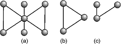
Figure 12: A network such as that in (a) includes several subgraphs, such as cycles (b) and trees (c).

12.1 Network Motifs

Network motifs are subgraphs that appear more frequently in a real network than could be statistically expected [147, 148, 149] (see Figure 13). Figure 14 shows some possible motifs of directed networks and their conventional names. To find the motifs in a real network, the number of occurrences of subgraphs in the network is compared with the expected number in the ensemble of networks with the same degree for each vertex. A large number of randomized networks from this ensemble is generated in order to compute the statistics of occurrence of each subgraph of interest. If the probability of a given subgraph to appear at least the same number of times as in the real network is smaller than a given threshold (usually $0.01$), the subgraph is considered a motif of the network.

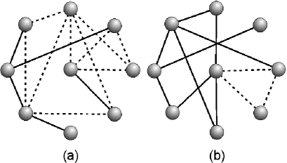
Figure 13: In a real network (a), the number of motifs (represented here by three vertices linked by dashed lines) is greater than in an equivalent random network (b).

Figure 14: Some types of motifs: (a) three-vertex feedback, (b) three chain, (c) feed-forward loop, (d) bi-parallel, (e) four-vertex feedback, (f) bi-fan, (g) feedback with two mutual dyads, (h) fully connected triad and (i) uplinked mutual dyad.

In order to quantify the significance of a given motif, its $Z$-score can be computed. If $N^{(\mathrm{real})}_{i}$ is the number of times that a motif $i$ appears in the real network, $\langle N^{(\mathrm{rand})}_{i}\rangle$ the ensemble average of its number of occurrences, and $\sigma^{(\mathrm{rand})}_{i}$ the standard deviation of the number of occurrences, then:

$$Z_{i}=\frac{N^{(\mathrm{real})}_{i}-\langle N^{(\mathrm{rand})}_{i}\rangle}{\sigma^{(\mathrm{rand})}_{i}}.$$ (76)

It is also possible to categorize different networks by the $Z$-scores of their motifs: networks that show emphasis on the same motifs can be considered as part of the same family [150]. For this purpose, the significance profile of the network can be computed. The significance profile is a vector that, for each motif of interest $i$, is used to compute the importance of this motif with respect to other motifs in the network:

$$\mathit{SP}_{i}=\frac{Z_{i}}{\sum_{j}Z_{j}^{2}}.$$ (77)

It is interesting to note that motifs are related to network evolution. As described by Milo et al. [148], different kinds of networks present different types of motifs e.g., for transcription networks of Saccharomyces cerevisiae and Escherichia coli two main motifs are identified: feed-forward loop and bi-fan; for neurons: feed-forward loop, bi-fan and bi-parallel; for food-webs: three chain and bi-parallel; for electronic circuits: feed-forward loop, bi-fan, bi-parallel, four-node feedback and three node feedback loop; and for the WWW: feedback with two mutual dyads, fully connected triad and uplinked mutual dyad. Thus, motifs can be considered as building blocks of complex networks and many papers have been published investigating the functions and evolution of motifs in networks [15].

12.2 Subgraphs and Motifs in Weighted Networks

In weighted networks, a subgraph may be present with different values for the weights of the edges. Onnela et al. [72] suggested a definition for the intensity of a subgraph based on the geometric mean of its weights on the network. Given a subgraph $g$, its intensity is defined by

$$I(g)=\left(\prod_{(i,j)\in\mathcal{E}(g)}w_{ij}\right)^{1/n_{g}},$$ (78)

where $n_{g}=|\mathcal{E}(g)|$ is the number of edges of subgraph $g$.

In order to verify whether the intensity of a subgraph is small because all its edges have small weight values or just one of the weights is too small, the coherence of the subgraph $\Psi$, defined as the ratio between geometric and arithmetic mean of its weights, can be used:

$$\Psi(g)=\frac{I(g)n_{g}}{\sum_{(i,j)\in\mathcal{E}(g)}w_{ij}}.$$ (79)

All possible subgraphs of the weighted graph can be categorized into sets of topologically equivalent subgraphs. Let $M$ be one such set of topologically equivalent subgraphs. The intensity of $M$ is given by $I_{M}=\sum_{g\in M}I(g)$ and its coherence by $\Psi_{M}=\sum_{g\in M}\Psi(g)$. An intensity score $ZI_{M}$ can be accordingly defined by

$$ZI_{M}=\frac{I_{M}-\langle I_{M}^{\mathrm{(rand)}}\rangle}{\sigma_{I_{M}}^{\mathrm{(rand)}}}$$ (80)

and the coherence score,

$$Z\Psi_{M}=\frac{\Psi_{M}-\langle\Psi_{M}^{\mathrm{(rand)}}\rangle}{\sigma^{\mathrm{(rand)}}_{\Psi_{M}}},$$ (81)

where $\langle I_{M}^{\mathrm{(rand)}}\rangle$ and $\sigma_{I_{M}}^{\mathrm{(rand)}}$ are the mean and the standard deviation of the intensities in a randomized graph ensemble; $\langle\Psi_{M}^{\mathrm{(rand)}}\rangle$ and $\sigma_{\Psi_{M}}^{\mathrm{(rand)}}$ are the average and the standard deviation of the coherence in the randomized ensemble. When the network is transformed to its unweighted version, $ZI_{M}$ and $Z\Psi_{M}$ tend to $Z$ (see Eq. (76)).

12.3 Subgraph Centrality

A way to quantify the centrality of a vertex based on the number of subgraphs in which the vertex takes part has been proposed [151]. The respective measurement, called subgraph centrality, considers the number of subgraphs that constitute a closed walk starting and ending at a given vertex $i$, with higher weights given to smaller subgraphs. This measurement is related to the moments of the adjacency matrix, Eq. (61):

$$\mathit{SC}_{i}=\sum_{k=0}^{\infty}\frac{(A^{k})_{ii}}{k!},$$ (82)

where $(A^{k})_{ii}$ is the $i$th diagonal element of the $k$th power of the adjacency matrix $A$, and the factor $k!$ assures that the sum converges and that smaller subgraphs have more weight in the sum. Subgraph centrality can be easily computed [151] from the spectral decomposition of the adjacency matrix,

$$\mathit{SC}_{i}=\sum_{j=1}^{N}v_{j}(i)^{2}e^{\lambda_{j}},$$ (83)

where $\lambda_{j}$ is the $j$th eigenvalue and $v_{j}(i)$ is the $i$th element of the associated eigenvector. This set of eigenvectors should be orthogonalized. The subgraph centrality of a graph is given by [95]:

$$\mathit{SC}=\frac{1}{N}\sum_{i=1}^{N}{\mathit{SC}_{i}}=\frac{1}{N}\sum_{i=1}^{N}{e^{\lambda_{i}}}.$$ (84)

13 Hierarchical Measurements

Using concepts of mathematical morphology [152, 153, 154, 155], it is possible to extend some of the traditional network measurements and develop new ones [156, 157, 158]. Two fundamental operations of mathematical morphology are dilation and erosion (see Figure 15). Given a subgraph $g$ of a graph $G$, the complement of $g$, denoted $\overline{g}$, is the subgraph implied by the set of vertices in $G$ that are not in $g$,

$$\mathcal{N}(\overline{g})=\mathcal{N}(G)\setminus\mathcal{N}(g)$$

($\setminus$ is the operator of set difference). The dilation of $g$ is the subgraph $\delta(g)$ implied by the vertices in $g$ plus the vertices directly connected to a vertex in $g$. The erosion of $g$, denoted $\varepsilon(g)$, is defined as the complement of the dilation of the complement of $g$:

$$\varepsilon(g)=\overline{\delta(\overline{g})}.$$

These operations can be applied repeatedly to generate the $d$-dilations and $d$-erosions:

$$\delta_{d}(g) = \underbrace{\delta(\delta(...(g)...))}_{d},$$ (85)

$$\varepsilon_{d}(g) = \underbrace{\varepsilon(\varepsilon(...(g)...))}_{d}.$$ (86)

The first operation converges to the entire network $G$ and the second converges to an empty network.

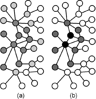
Figure 15: Example of morphological operations: (a) Dilation: the dilation of the initial subnetwork (dark gray vertices) corresponds to the dark and light gray vertices; (b) Erosion: the erosion of the original subnetwork, given by the dark gray vertices in (a), results in the subnetwork represented by the black vertices in (b).

The $d$-ring of subgraph $g$, denoted $R_{d}(g)$, is the subgraph implied by the set of vertices

$$\mathcal{N}(\delta_{d}(g))\setminus\mathcal{N}(\delta_{d-1}(g));$$

the $rs$-ring of $g$, denoted $R_{rs}(g)$, is the subgraph implied by

$$\mathcal{N}(\delta_{s}(g))\setminus\mathcal{N}(\delta_{r-1}(g)).$$

Note that $R_{d}(g)=R_{dd}(g).$ The same definitions can be extended to a single vertex considering the subgraph implied by that vertex, and to an edge considering the subgraph formed by the edge and the two vertices that it connects. In the case of a single vertex $i$ the abbreviations $R_{d}(i)$ and $R_{rs}(i)$ are used. For example, in Figure 16, $R_{1}(15)$ includes the vertices $\{8,14,16,17\}$; $R_{2}(15)$ includes $\{1,13,18,19\}$; for the graph $g$ implied by the vertices $\{1,15,22\}$ (in black), $R_{1}(g)$ includes the vertices in white: $\{2,3,4,5,6,7,8,9,14,16,17\}$.

The hierarchical degree of a subgraph $g$ at distance $d$, henceforth represented as $k_{d}(g)$, can be defined as the number of edges connecting rings $R_{d}(g)$ to $R_{d+1}(g)$. Note that $k_{0}(i)$ is equal to $k_{i}$.

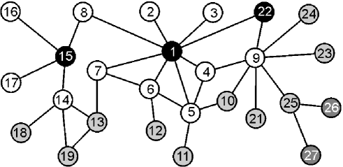
Figure 16: The subgraph of interest is defined by black vertices, $g=\{1,15,22\}$. The first hierarchical level of $g$ is given by the first dilation around $g$, represented by the white vertices; the second hierarchical level is obtained dilating the subnetwork again, represented by the gray vertices. The hierarchical degree of the first level is given by the number of edges from white to light gray vertices, $k_{1}(g)=12$, and the hierarchical degree of the second level is the number of edges from light gray to dark gray vertices, $k_{2}(g)=2$.

Another measurement which can be hierarchically extended is the clustering coefficient. The $rs$-clustering coefficient of $g$, $C_{rs}(g)$, can be defined as the number of edges in the respective $rs$-ring $n_{rs}$, divided by the total of possible edges between the vertices in that ring, i.e. for undirected networks

$$C_{rs}(g)=\frac{2n_{rs}(g)}{|\mathcal{N}(R_{rs}(g))|(|\mathcal{N}(R_{rs}(g))|-1)}.$$ (87)

Other possible hierarchical measurements are briefly described in the following. The convergence ratio at distance $d$ of subgraph $g$, $\mathit{cv}_{d}(g)$, corresponds to the ratio between the hierarchical subgraph degree at distance $d-1$ and the number of vertices in the ring at distance $d$; it can be understood as the average number of edges received by each vertex in the hierarchical level $d$ from the previous level,

$$\mathit{cv}_{d}(g)=\frac{k_{d-1}(g)}{|\mathcal{N}(R_{d}(g))|}.$$ (88)

It is also possible to define the divergence ratio, which corresponds to the reciprocal of the convergence ratio

$$\mathit{dv}_{d}(g)=\frac{|\mathcal{N}(R_{d}(g))|}{k_{d-1}(g)}.$$ (89)

The intra-ring degree is obtained by taking the average among the degrees of vertices in the subnetwork $R_{d}(g)$; note that only internal ring edges are considered. On the other hand, the inter-ring degree is defined by the average number of connections between vertices in ring $R_{d}(g)$ and those in $R_{d+1}(g)$.

14 Fractal Dimensionality

Fractals are objects or quantities that display self-similarity (or self-affinity) in all scales. For complex networks, the concept of self-similarity under a length-scale transformation was not expected because of the small world property, implying the average shortest path length of a network increases logarithmically with the number of vertices. However, Song et al. [159] analyzed complex networks by using fractal methodologies and verified that real complex networks may consist of self-repeating patterns on all length scales.

In order to measure the fractal dimension of complex networks, a box counting method and a cluster growing method has been proposed [159]. In the former, the network is covered with $N_{B}$ boxes, where all vertices in each of them are connected by a minimum distance smaller than $l_{B}$. $N_{B}$ and $l_{B}$ are found to be related by

$$N_{B}\sim l_{B}^{-d_{B}},$$ (90)

where $d_{B}$ is the fractal box dimension of the network.

For the cluster growing method, a seed vertex is chosen at random and a cluster is formed by vertices distant at most $l$ from the seed. This process is repeated many times and the average mass of resulting clusters is calculated as a function of $l$, resulting in the relation

$$\langle M_{c}\rangle\sim l^{d_{f}},$$ (91)

where the average mass $\langle M_{c}\rangle$ is defined as the number of vertices in the cluster and $d_{f}$ is the fractal cluster dimension.

For a network whose vertices have a typical number of connections, both exponents are the same, but this is not the case for scale-free networks.

Another scaling relation is found with a renormalization procedure based on the box counting method [159]. A renormalized network is created with each box of the original network transformed into a vertex and two new vertices are connected if at least one edge exists between vertices of the corresponding boxes in the original network. By considering the degree $k^{\prime}$ of each vertex of the renormalized network versus the maximum degree $k$ in each box of the original network we have that:

$$k^{\prime}\approx l_{B}^{-d_{k}}k,$$ (92)

The exponents $\gamma$ (of the power law of the degree distribution), $d_{B}$ and $d_{k}$ are related by [159]:

$$\gamma=1+d_{B}/d_{k}.$$ (93)

Thus, scale-free networks, characterized by the exponent $\gamma$, can also be described by the two length invariant exponents $d_{B}$ and $d_{k}$.

15 Other measurements

This section describes additional, complementary measurements related to network complexity, edge reciprocity and matching index.

15.1 Network Complexity

It might be of interest to quantify the ‘complexity’ of a network. Lattices and other regular structures, as well as purely random graphs, should have small values of complexity. Some recent proposals are briefly presented below.

Machta and Machta [160] proposed the use of the computational complexity of a parallel algorithm [161] for the generation of a network as a complexity measurement of the network model. If there is a known parallel algorithm for the generation of the network of order $\mathcal{O}(f(N))$, with $f(x)$ a given function, then the complexity of the network model is defined as $\mathcal{O}(f(N))$. For example, Barabási-Albert networks can be generated in $\mathcal{O}(\log\log N)$ parallel steps [160].

Meyer-Ortmanns [162] associated the complexity of the network with the number of topologically non-equivalent graphs generated by splitting vertices and partitioning the edges of the original vertex among the new vertices, the transformations being restricted by some constraints to guarantee the generation of valid graphs.

The off-diagonal complexity, proposed by Claussen [163] is defined as an entropy of a specially defined vertex-vertex edge correlation matrix. An element with indexes $(k,l)$ of this matrix has contributions from all edges that connect a vertex of degree $k$ to a vertex of degree $l$ (only values $k>l$ are used).

15.2 Edge Reciprocity

For directed networks, it is often interesting to know if their edges are reciprocal, i.e. if vertex $i$ is linked to vertex $j$, is vertex $j$ also linked to vertex $i$? Such information helps to obtain a better characterization of the network, can be used to test network models against real networks and gives indication of how much information is lost when the direction of the edges is discarded (e.g. for the computation of some measurements that only apply to undirected networks).

A standard way to obtain information about reciprocity is to compute the fraction of bilateral edges:

$$\varrho=\frac{\sum_{ij}a_{ij}a_{ji}}{M},$$ (94)

where $M$ is the total number of edges.

A problem with this measurement is that its value is only relevant with respect to a random version of the network, as networks with higher connectivity tend to have a higher number of reciprocal edges due exclusively to random factors. Garlaschelli and Loffredo [164] proposed the use of the correlation coefficient of the adjacency matrix:

$$\rho=\frac{\sum_{ij}(a_{ij}-\bar{a})(a_{ji}-\bar{a})}{\sum_{ij}(a_{ij}-\bar{a})^{2}},$$ (95)

where $\bar{a}$ is the mean value of the elements of the adjacency matrix. This expression, known as edge reciprocity, simplifies to

$$\rho=\frac{\varrho-\bar{a}}{1-\bar{a}}.$$ (96)

This value is an absolute quantity, in the sense that values of $\rho$ greater than zero imply larger reciprocity than the random version (reciprocal networks), while values below zero imply smaller reciprocity than a random network (antireciprocal networks). This concept can be easily extended to weighted networks by substituting $a_{ij}$ for $w_{ij}$ in the above expressions.

15.3 Matching Index

A matching index can be assigned to each edge in a network in order to quantify the similarity between the connectivity of the two vertices adjacent to that edge [165]. A low value of the matching index identifies an edge that connects two dissimilar regions of the network, thus possibly playing an important role as a shortcut between distant network regions [165]. The matching index of edge $(i,j)$ is computed as the number of matching connections of vertices $i$ and $j$ (i.e. connections to the same other vertex $k$), divided by the total number of connections of both vertices (excluding connections between $i$ and $j$),

$$\mu_{ij}=\frac{\sum_{k\neq i,j}a_{ik}a_{jk}}{\sum_{k\neq j}a_{ik}+\sum_{k\neq i}a_{jk}}.$$ (97)

For directed networks, matching connections are only those in the same direction, and incoming and outgoing connections of vertices $i$ and $j$ should be considered separately. The matching index has also been adapted to apply to consider all the immediate neighbors of a node, instead of a single edge [166].

16 Measurements of Network Dynamics and Perturbation

This section covers two important related issues, namely the use of trajectories to characterize the dynamical evolution of complex networks connectivity and a brief discussion about the sensitivity of measurements to perturbations.

16.1 Trajectories

As motivated in the Introduction of this work, in the following we analyze the behavior of trajectories (see Figure 17) defined by tuples of measurements as the analyzed network undergoes progressive modification, such as during their growth. The network models considered for the illustration of trajectories include: Erdős-Rényi random graphs (ER), random networks with community structure (CN), Watts-Strogatz small-worlds (WS), Geographical Networks (GN), and Barabási and Albert scale-free networks (BA) (see section 3 for a description of these models). The number of vertices considered was $250,500,1000$ and $2000$, and the number of edges varies so that the average vertex degree ranges from $4$ to $204$, increasing by steps of $20$. In the case of the GN model, the vertices were randomly distributed through a square box of unit size. The $\lambda$ parameter in Eq. 12 was adjusted in order to guarantee the desired average degree. The CN networks include four communities interconnected by using $p_{\mathrm{out}}/p_{\mathrm{in}}$ (see Section 3) equal to $5\%$, $10\%$ and $15\%$. In the WS model, the probability $p$ of rewiring the edges was $0.0002$, $0.02$ and $0.1$. For the sake of better visualization, the trajectories of the WS and CN models are drawn separately from the other cases. The direction of evolution of the trajectories as more edges are included is indicated by arrows in Figures 17. These results are discussed subsequently with respect to several pairs of measurements.

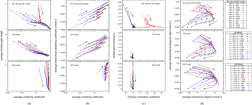
Figure 17: Trajectories defined by pairs of measurements. Each point corresponds to $10$ network model realizations. Network sizes used are $250,500,1000,$ and $2000$; average degrees vary from $4$ to $204$ in steps of $20$; for the community model, $p_{\mathrm{out}}/p_{\mathrm{in}}$ is $5\%,10\%,$ and $15\%$; for the WS model the rewiring probability values are $0.0002,0.02,$ and $0.1$.

16.1.1 Average Clustering Coefficient and Average Shortest Path Length

By inspecting the trajectories associated to this pair of measurements (see Figure 17(a)), two distinct behaviors can be identified. First, the average clustering coefficient $\widetilde{C}$ exhibits a high variation while the average shortest path length $\ell$ remains almost constant with addition of edges for the ER, CN and BA models. Second, an opposite effect is observed for GN and WS models. In the latter case, the $\ell$ value undergoes a steep decrease, while staying almost constant for the other network models. This effect is related to the fact that GN and WS models are formed by vertices that tend to link to closer neighbors. Hence, with the addition of edges some long-range connections may decrease $\ell$ while $\widetilde{C}$ remains almost unchanged. Furthermore, $\ell$ decreases faster for WS model than for GN while $\widetilde{C}$ for the former model remains larger than in the other cases. This can be explained by the fact that the WS model is more regular than the GN and has larger $\widetilde{C}$.

In the case of ER, CN and BA models, the values of $\ell$ and $\widetilde{C}$ are smaller than for the other models. For $\ell$ the connections are not limited by proximity, adjacency or geography, and for $\widetilde{C}$ loops of order three appear when new edges are added to them, increasing this measurement.

Another interesting fact observed from Figure 17(a) is that all curves converge to the same point, corresponding to fully connected graphs, as the networks become denser. Therefore, $\ell$ and $\widetilde{C}$ tend in this stage to a unit value.

16.1.2 Average Clustering Coefficient and Average Hierarchical Clustering Coefficient of Second Level

The combination of $\widetilde{C}$ and the average hierarchical clustering coefficient of second level $\langle C_{2}(i)\rangle$, where the average is taken over all vertices in the network, see Figure 17(b), tend to follow a power law for all trajectories except for the GN and WS models, whose curves have a minimum value for $\langle C_{2}(i)\rangle$. Nonetheless, the highest growth rate is observed for the trajectories of WS model after their minimum value of $\langle C_{2}(i)\rangle$ is reached.

Another interesting characteristic of this combination of measurements is that $\widetilde{C}$ is greater than $\langle C_{2}(i)\rangle$. This can be explained by the fact of $\langle C_{2}(i)\rangle$ is related to the presence of loops of order five without additional connections between their vertices [158]. Since loops of higher orders are less likely to appear in the considered networks, $\widetilde{C}$ is larger than $\langle C_{2}(i)\rangle$.

16.1.3 Pearson Correlation Coefficient and Central Point Dominance

For all network models, except for the GN, the $r$ value is close to zero even with the addition of new edges, as can be seen in Figure 17(c), which shows the trajectories defined by the pair of measurements Pearson correlation of the degrees $r$ (Section 6) and central point dominance $\mathit{CPD}$ (Section 9) as the average degree increases. This property can be explained by the fact that in ER, CN and WS models edges are placed without regard to vertex degree, while the BA model is based on growth [83], which leads to non-assortative mixing (i.e. no correlation between vertex degrees). The $r$ value for the GN model is greater than zero in almost all cases because its growing dynamics is based on the geographic proximity of vertices. As the position of vertices is randomly chosen, some regions may result highly populated, implying the respective vertices to have a high probability of becoming highly interconnected. On the other hand, vertices belonging to the regions barely populated have a small likelihood to become “hubs” while still having a good chance of being connected. These two opposite behaviors lead to a $r$ value greater than zero.

The central point dominance is a measurement of the maximum betweenness of any point in the network [108] (see Section 9 for further details). By observing Figure 17(c), one can see that most network models exhibit average values of this measurement close to zero, except for the BA, GN and WS cases. In BA networks, values significantly larger than zero only occur in the beginning of the growth process (i.e. with few edges).

For WS models, the way in which they are normally constructed (see Section 3) directly contributes to producing a network with modular structure, hence a high $\mathit{CPD}$ value. Nevertheless, when new edges are added, the network gets denser and the value of this measurement goes to zero. In CN models, the $\mathit{CPD}$ coefficient depends on the relation between the average vertex degrees inside and outside communities, i.e. when the network is highly modular, the $\mathit{CPD}$ value tends to become larger.

16.1.4 Average Hierarchical Degree of Second Level and Average Hierarchical Divergence Ratio of Third Level

As shown in Figure 17(d), all curves obtained for the average hierarchical degree of second level $\langle k_{2}(i)\rangle$ and the average hierarchical divergence ratio of level three $\langle\mathit{dv}_{3}(i)\rangle$ have similar behavior. When the networks are sparse and new edges are added to them increasing the average vertex degree, the average hierarchical counterpart increases until a maximum value. Afterwards, since the networks have a finite size, further increase of the connectivity tends to reduce the number of hierarchical levels in the networks and, as consequence, the average hierarchical vertex degree of levels higher than one tends to decrease. The hierarchical divergence ratio of level three decreases with larger average vertex degree.

16.1.5 Discussion

As presented in Figure 17, each measurement is specifically sensitive to the effects of addition of new edges to a network. Interestingly, the sensitivity also depend strongly on the network model. Some trajectories resulted closer one another for specific network models as a consequence of inherent structural similarities. This effect is particularly pronounced in trajectories defined by the average clustering coefficient and average shortest path length, where two classes of trajectories appear, one for ER, BA and CN, and another for GN and WS.

The analysis of network dynamics provides insights about model similarities. If network trajectories evolve in a similar fashion, it is possible to infer that these networks have similar structure concerning the respective pair of measurements. However, for other measurements, this similarity may be weaker or non-existent. For instance, in the space defined by the average clustering coefficient and average shortest path length, the curves obtained for RA and BA evolve in similar fashion. This behavior is not observed in the space defined by the central point dominance and Pearson correlation coefficient. Also, by inspecting the trajectories, it is possible to determine the correlation between measurements during the network evolution. For instance, the dynamics of the average clustering coefficient and the average hierarchical clustering coefficient of second level present correlation for ER and CN.

The trajectory-based study described here can be immediately extended to real network analysis and modeling. In the case of the WWW, for instance, by inspecting its evolution in the measurements space it is possible to develop more precise models to represent and characterize its structure. For citation networks, it is possible to characterize the networks generated for different knowledge areas and obtain insights about their structure and evolution. All in all, trajectories provide a visually clear and accessible interpretation and dynamics about the evolution of complex networks connectivity.

16.2 Perturbation Analysis

Another important property of a given measurement relates to how much it changes when the networks undergo small perturbations (e.g., rewiring, edge or vertex attack, weight changes, etc.). For instance, the shortest path length provides a good example of a particularly sensitive measurement, in the sense that the modification of a single connection may have great impact in its value. The quantification of the sensitivity of measurements to different types of perturbations and networks therefore provides valuable information to be considered for characterization, analysis and classification of complex networks.

Interesting insights can be obtained as far as this subject is concerned by performing progressive perturbations in a specific network and observing the respective relative variations in the measurement of interest. Figure 18 shows the trajectories obtained in the $\{\widetilde{C},\ell\}$ and $\{\widetilde{C},\mathit{CPD}\}$ feature spaces shown in Figure 18(a) and (b), respectively, while considering edge randomization [54] (see also Section 3.3) progressively performed for the BA, ER, GN and WS models ($N=1000$, $\langle k\rangle=6$). The values shown in this figure were normalized through division by the respective averages of the measurements in order to provide suitable visual comparison.

Figure 18: Example of perturbations. Each point corresponds to $100$ realizations of networks with $N=1000$ and $\langle k\rangle=6$.

Each successive point along the trajectories, which are indicated by arrows in Figure 18, was obtained after a number of rewirings which are successive integer powers of two (for the sake of obtaining more uniform visualization). It is clear from the results that the sensitivity of the two pairs of measurements varies substantially with respect to the type of network under consideration. More specifically, much wider variations were observed for the GN and WS models. The stable trajectories obtained for the shortest path length in the case of the BA model is a direct consequence of the fact that these networks are inherently characterized by low overall average shortest path length. A similar situation is verified for the clustering coefficient, which tends to be small in those two types of networks. The evolution of the trajectory regarding the clustering coefficient and average shortest path length for the GN and WS networks is a direct consequence of the fact that the progressive edge rewiring tend to strongly reduce those two measurements. The marked difference of sensitivity of measurements to perturbations depending on the type of network model suggests that quantifications of the sensitivity (e.g. the standard deviation or entropy) can be potentially useful as measurements for network identification.

17 Correlations Analysis

In order to investigate possible linear relationships between several of the measurements considered, we calculated them for the BA, ER and GN models ($N=1000$ and $\left<k\right>=4$) and estimated the respective pairwise correlations. Table 3 shows the values obtained with respect to each model and also considering all models together (‘All’).

Table 3: Correlation between measurements for the BA, ER and GN models and “All” jointly. Values estimated from $1000$ realizations (for each model) of networks with $N=1000$ and $\langle k\rangle=4$.

		$\mathit{st}$	$r$	$\widetilde{C}$	$\ell$	$\mathit{CPD}$	$\langle k_{2}(i)\rangle$	$\langle C_{2}(i)\rangle$	$\langle\mathit{dv}_{3}(i)\rangle$
	BA	1.00
$\mathit{st}$	ER	1.00
	GN	1.00
	All	1.00
	BA	-0.22	1.00
$r$	ER	-0.01	1.00
	GN	-0.13	1.00
	All	0.71	1.00
	BA	0.06	-0.29	1.00
$\widetilde{C}$	ER	-0.01	0.07	1.00
	GN	0.04	-0.00	1.00
	All	0.31	0.82	1.00
	BA	-0.01	0.38	-0.63	1.00
$\ell$	ER	-0.06	0.04	-0.08	1.00
	GN	-0.10	0.02	0.03	1.00
	All	0.69	0.96	0.88	1.00
	BA	-0.09	0.23	0.39	-0.58	1.00
$\mathit{CPD}$	ER	-0.61	0.10	0.03	0.07	1.00
	GN	-0.05	-0.02	0.03	0.23	1.00
	All	-0.87	-0.44	0.02	-0.41	1.00
	BA	0.01	-0.30	0.63	-0.99	0.60	1.00
$\langle k_{2}(i)\rangle$	ER	0.04	0.03	0.08	-0.90	-0.06	1.00
	GN	0.08	0.28	-0.02	-0.65	-0.13	1.00
	All	-0.96	-0.80	-0.43	-0.79	0.85	1.00
	BA	0.02	0.02	0.58	-0.74	0.59	0.76	1.00
$\langle C_{2}(i)\rangle$	ER	-0.03	0.04	0.45	-0.16	0.02	0.19	1.00
	GN	-0.00	0.09	0.59	0.18	0.07	-0.11	1.00
	All	0.37	0.86	0.99	0.91	-0.05	-0.49	1.00
	BA	0.01	0.26	-0.57	0.91	-0.52	-0.94	-0.69	1.00
$\langle\mathit{dv}_{3}(i)\rangle$	ER	0.03	-0.10	-0.01	-0.25	-0.01	-0.16	-0.04	1.00
	GN	-0.02	-0.28	-0.09	-0.03	-0.00	-0.50	-0.21	1.00
	All	-0.14	-0.74	-0.97	-0.79	-0.18	0.27	-0.96	1.00

Several interesting facts can be inferred from this table. First, particularly high absolute values of correlations have been obtained for the BA model, with low absolute values observed for the ER and GN cases. This seems to represent a particularly interesting property of the BA networks. Another interesting finding regards the fact that the correlations obtained for specific network models not necessarily agree with that obtained when the three models are considered together. This is the case, for instance, of the low correlation observed between the measurement average shortest path length $\ell$ and log-log degree distribution straightness $\mathit{st}$ for each of the three individual models and high correlation otherwise obtained when these three models are considered jointly. This interesting behavior can be immediately understood from Figure 19, which indicates that the three low correlations groups obtained for the individual models tend to align globally, therefore implying the relatively strong negative correlation. Such situations indicate that the individual and global correlations provide information about different types of relationships and should be treated accordingly.

Figure 19: Example of scatterplot showing the low correlation between log-log degree density straightness and the average shortest path length for all the individual models and the high correlation for all models together. The networks have $N=1000$ and $\langle k\rangle=4$; $500$ realizations of each model were used.

It is also clear from the results in Table 3 that particularly high correlations were obtained between the average shortest path length $\ell$ and the vertex degree at the second hierarchical level $\langle k_{2}(i)\rangle$. This fact suggests that this specific hierarchical vertex degree may be considered, at least for the three types of networks, as an estimation of the average shortest path length, allowing substantial computational saving. Another interesting result is that the highest correlations were obtained for the BA model, a possible consequence of the respective hubs. For instance, the correlation between the average shortest path length and the average clustering coefficient was equal to -0.63 for the BA models. This is a consequence of the fact that additional links tend to be established with the hubs and therefore contribute to higher clustering and shortest paths.

18 Multivariate Statistical Methods for Measurement Selection and Network Classification

The intrinsic statistical variability of the connectivity of real and simulated complex networks, even when produced by the same process or belonging to the same class, implies that sound characterization, comparison and classification of networks should take into account not only the average measurements, but also additional information about their variability including higher statistical moments (e.g., variance, kurtosis, etc.) as well as multivariate statistical distribution of the measurements. For example, realizations obtained by using the Barabási-Albert (BA) model with fixed parameters will produce networks which, though not identical, will have equivalent statistical distribution of their properties. Figures 20 shows a scatterplot obtained by considering 1000 realizations of the BA model with $N=1000$ and $m=3$ with respect to the measurements $(r,\widetilde{C},\ell)$, where $r$ is the Pearson correlation coefficient of vertex degrees; $\widetilde{C}$, the average clustering coefficient; and $\ell$, the average shortest path length. Although the obtained points form a well-defined cluster around the average point $(-0.0653,\,0.0365,\,3.255)$, there is a significant dispersion of cases around this center, implying that additional measurements other than the mean need to be used for proper characterization of the network under analysis. Therefore, any objective attempt at characterizing, comparing or classifying complex networks needs to take into account distributions in phase spaces such as that in Figure 20. Such an important task can be effectively accomplished by using traditional and well-established concepts and methods from Multivariate Statistics (e.g., [39, 40],McLachlan:04) and Pattern Recognition (e.g., [39, 167, 40]).

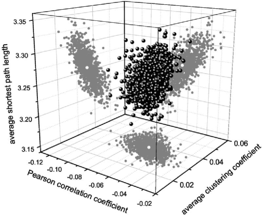
Figure 20: The spatial distribution in the $(r,\widetilde{C},\ell)$ phase space of $1000$ different realizations of the BA model with $N=1000$ and $m=3$. The distribution has been projected into the three main planes (gray shadows) for the purpose of better visualization. The white circles in the middle of the gray shadows represent the mean projected into these planes.

As far as the choice and interpretation of network measurements are concerned, two multivariate methods stand out as being particularly useful, namely Principal Component Analysis — PCA (e.g. [39, 40]) and Canonical Variable Analysis (e.g., [168]). While the former procedure allows the reduction of the dimensionality of the measurement phase space, obtained in terms of projections so as to concentrate the variation of the data along the first axes (i.e. those associated to the highest covariance matrix eigenvalues), the second method implements such projections so as to achieve best separation, in terms of inter and intra-class distances (see below), between the involved classes of networks under analysis.

Another situation in multivariate statistics which is particularly important for complex network research concerns network identification. Indeed, it is often a critical issue to decide to which of several models a given theoretical or experimentally obtained network belongs. This important problem can be approached in a sound way by using Bayesian decision theory [40], a well-established methodology which, provided we have good probabilistic models of the properties of the networks, allows near-optimal classification performance .

The current section presents and illustrates in a self-contained and accessible fashion these two families of methods from multivariate statistics, i.e. dimensionality reduction (PCA and canonical analysis) and classification (Bayesian decision theory). The possibility to apply Bayesian decision theory on phase spaces obtained through canonical variable analysis projections of multidimensional measurement spaces is also illustrated. The potential for applications of these methods is illustrated with respect to three reference complex network models — namely Erdős and Rényi random graph (ER), Barabási-Albert (BA) and Geographical Network model (GN), against which some real-world networks are classified.

It should be observed that many other methods from multivariate statistical analysis, including hierarchical clustering and structural equation modeling, can also be valuable for investigations in complex network research. Though the potential of hierarchical clustering for suggesting relationships between the classes is briefly illustrated in the following, further information about such methods can be found in textbooks such as [167, 40, 39, 169, 170, 168].

18.1 Principal Component Analysis

Let the connectivity properties of a set of $R$ complex networks, irrespective of their type or origin, be described in terms of $P$ scalar measurements $x_{i}$, $i=1,2,\ldots,P$, organized as the feature vector $\vec{x}=(x_{1},x_{2},\ldots,x_{P})^{T}$. The covariance matrix $K$ can be estimated as

$$K=\frac{(\vec{x}-\vec{\left<x\right>})(\vec{x}-\vec{\left<x\right>})^{T}}{R},$$ (98)

where $\vec{\left<x\right>}$ is the average feature vector, each element of which corresponds to the average of the respective measurement. As $K$ is a real and symmetric $P\times P$ matrix, a set of $P$ decreasing eigenvalues $\lambda_{i}$ and respectively associated eigenvectors $\vec{v_{i}}$ can be obtained. Moreover, if all eigenvalues are distinct, the eigenvectors will be orthogonal . These eigenvectors can be stacked to obtain the transformation matrix $T$, i.e.

$$T=\left[\begin{array}[]{ c }\leftarrow\vec{v_{1}}\rightarrow\\ \leftarrow\vec{v_{2}}\rightarrow\\ \ldots\\ \leftarrow\vec{v_{P}}\rightarrow\end{array}\right].$$ (99)

The original feature vectors $\vec{x}$ can now be transformed into a new coordinates reference through the following linear transformation corresponding to axes rotation:

$$\vec{X}=T\vec{x}$$ (100)

which defines the principal component projections.

It can be shown [170] that the distribution of points in the new phase space obtained by the above transformation is such that the largest variance is observed along the first axis, followed by decreasing variances along the subsequent axes, with the initial axes called principal. Such an important property allows, by considering only the principal eigenvalues, the original cloud of points to be projected along phase spaces of a smaller dimension $p$. In order to do so, the transformation matrix is constructed while taking into account only the first $T_{p}$ eigenvectors associated to the largest eigenvalues, i.e.

$$T_{p}=\left[\begin{array}[]{ c }\leftarrow\vec{v_{1}}\rightarrow\\ \leftarrow\vec{v_{2}}\rightarrow\\ \ldots\\ \leftarrow\vec{v_{p}}\rightarrow\end{array}\right].$$ (101)

Figure 21: The principal component projection of the distribution of measurements in Figure 20. Measurement values were first normalized by subtracting the corresponding mean value and dividing by the standard deviation, to avoid distortions due to the different absolute values. The first and second PCA variable have projecting vectors $(-0.005,0.707,-0.707)$ and $(0.006,0.707,0.707)$ in the space defined by $(r,\widetilde{C},\ell)$, respectively.

Figure 21 shows the effect of projecting the cloud of points in Figure 20 onto the two main axes where the variance of the samples is maximized. Although useful for implementing dimensionality reduction — which favors visualization, redundancy reduction, and computational savings — the principal component analysis method is limited as it does not explicitly consider the category of each individual. This limitation is overcome by the canonical variable analysis described below. Note that the obtained projections are little influenced by the measurement $r$, which is compatible with the fact that degree correlations are almost absent in BA networks [24].

18.2 Canonical Variable Analysis

The method known as canonical variable analysis provides a powerful extension of principal component analysis by performing projections which optimize the separation between the known categories of objects. Before presenting the method, we introduce a series of scatter measurements considering each category separately and also all categories, from which the overall criterion for class separation is defined.

Let us consider that the $R$ complex networks of interest can be divided into $N_{c}$ classes, each one with $N_{i}$ objects and identified as $C_{i}$, $i=1,2,\ldots,N_{c}$, and that each object $\xi$ is represented by its respective feature vector $\vec{x_{\xi}}=(x_{1},x_{2},\ldots,x_{P})^{T}$ (see the previous section). The total scatter matrix, $S$, expressing the overall dispersion of the measurements [39] is defined as follows

$$S=\sum_{\xi\,=1}^{R}\left(\vec{x_{\xi}}-\vec{\left<x\right>}\right)\left(\vec{x_{\xi}}-\vec{\left<x\right>}\right)^{T}.$$ (102)

The scatter matrix for each class $C_{i}$ is given as

$$S_{i}=\sum_{\xi\in\;C_{i}}\left(\vec{x_{\xi}}-\vec{\left<x\right>}_{i}\right)\left(\vec{x_{\xi}}-\vec{\left<x\right>}_{i}\right)^{T},$$ (103)

where $\vec{\left<x\right>}_{i}$ is the average feature vector of the class $C_{i}$.

The intraclass scatter matrix, providing the dispersion inside each of the classes, is defined as

$$S_{\mathrm{intra}}=\sum_{i=1}^{N_{c}}S_{i}.$$ (104)

Finally, the interclass scatter matrix, characterizing the dispersion between each pair of classes, is given as

$$S_{\mathrm{inter}}=\sum_{i=1}^{N_{c}}N_{i}\left(\vec{\left<x\right>}_{i}-\vec{\left<x\right>}\right)\left(\vec{\left<x\right>}_{i}-\vec{\left<x\right>}\right)^{T}.$$ (105)

It can be verified that

$$S=S_{\mathrm{intra}}+S_{\mathrm{inter}}.$$ (106)

The objective of the canonical analysis method is to maximize the interclass dispersion while minimizing the intraclass scattering (e.g., [168]). This can be achieved through the following linear transformation

$$\vec{X_{\xi}}=\Gamma\vec{x_{\xi}}$$ (107)

where $\Gamma=[\vec{\gamma_{1}},\vec{\gamma_{2}},\ldots,\vec{\gamma_{p}}]^{T}$ is chosen so that $\vec{\gamma_{1}}$ maximizes the ratio

$$\frac{\vec{\gamma_{1}}^{T}S_{\mathrm{inter}}\vec{\gamma_{1}}}{\vec{\gamma_{1}}^{T}S_{\mathrm{intra}}\vec{\gamma_{1}}},$$ (108)

and $\vec{\gamma_{\xi}}$, $\xi=2,3,\ldots,p$, maximizes a similar ratio and

$$\vec{\gamma_{\xi}}^{T}S_{\mathrm{intra}}\vec{\gamma_{\xi}}=0.$$ (109)

It can be shown that the vectors $\vec{\gamma_{1}},\vec{\gamma_{2}},\ldots,\vec{\gamma_{\xi}}$ correspond to the eigenvectors of the matrix $S_{\mathrm{intra}}^{-1}S_{\mathrm{inter}}$.

Figure 22 illustrates a phase space (a) containing two distributions of observations, as well as the respective PCA (b) and canonical analysis (c) projections considering two dimensions. The potential of the canonical approach for obtaining separated clusters is evident from this example.

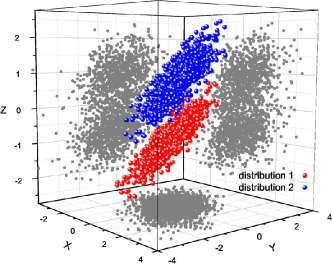
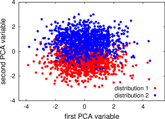
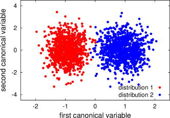
Figure 22: A phase space (scatterplot) containing two distributions of points (a) and respective PCA (b) and canonical (c) projections. Note that neither the projections into the three main planes (a) nor the PCA projection (b) separate the distributions, in contrast to the canonical projection (c).

18.3 Bayesian Decision Theory

The elegant and sound methodology known as Bayesian decision theory provides an intuitive and effective means for classifying objects into a given set of categories. In principle, it is assumed that the mass probabilities $P_{i}$, as well as the conditional probability densities, $p(\vec{x_{\xi}}|C_{i})$, are all given or can be properly estimated (e.g., by using parametric or non-parametric methods, see [40, 167, 39]). The mass probability $P_{i}$ corresponds to the probability that an object, irrespective of its properties, belongs to class $C_{i}$, and therefore can be estimated from the respective relative frequency. The conditional probabilities $p(\vec{x_{\xi}}|C_{i})$ provide a statistical model of how the measurements in the feature vectors are distributed inside each category. Given an object with unknown classification, the most likely category $c$ to be assigned to it is the one for which the respectively observed feature vector $\vec{x}$ produces the highest value of $P_{\xi}p(\vec{x}|C_{\xi})$. In case the probability functions are not available, it is still possible to use an approximate classification method, known as $k$-nearest neighbors (e.g. [40]), which consists in identifying the set of the $k$ individuals which are closer (i.e. smaller distance between feature vectors) to the sample to be classified, and take as the resulting category that corresponding to the most frequent class among the nearest neighbors.

Let us illustrate the above concepts and methodology in terms of a situation involving three categories $C_{1}$, $C_{2}$ and $C_{3}$ of complex networks, namely Geographical Network (GN), Watts-Strogatz small-world network (WS) and Erdős and Rényi random graph (ER), characterized in terms of their normalized average shortest path length $l$ and Pearson correlation coefficient of vertex degrees $r$. The corresponding scatterplot is shown in Figure 23(a).

Figure 23: A scatterplot of normalized measurements containing several complex networks derived from three main categories, i.e. Geographical Network (GN), Watts-Strogatz (WS) and Erdős and Rényi random graph (ER) models (a), and respective Gaussians and decision regions obtained by using the Bayes method considering parametric (b) and non-parametric (c) estimation. Network parameters are $N=250,\langle k\rangle=20$, with $1000$ realizations for each model; rewiring probability in the WS model is $0.4$.

Usually we do not know the mass and conditional probabilities of each type of networks, so they have to be estimated from the available data. This stage can be understood as the training phase of the Bayesian decision theory method. There are two main ways to estimate the probabilities required: parametric and non-parametric. In the former, the mathematical form of the probability functions is known (e.g., normal distribution) and the respective parameters (mean and covariance matrix, in the case of normal distributions) need to be estimated; in the latter, the mathematical type of the densities is unknown , being estimated, e.g., through some interpolation procedure such as the Parzen windows methodology [40]. Once the training phase is concluded, new objects whose classes are to be determined have their measurements estimated and used to identify, among the probability distributions of the trained models, which are the most likely respective classes. This categorization procedure corresponds to the decision phase of the Bayesian methodology.

Figure 23(b) illustrates the parametric approach, considering three normal density distributions, as applied to the data in Figure 23(a). These distributions were defined by having their parameters (namely average vector and covariance matrix) estimated from the respective experimental measurements. The separating frontiers are shown in the projection at the bottom of the figure. The decision regions obtained by using non-parametric estimation through Parzen windows is shown in Figure 23(c).

Note that a very high dimensional feature space implies that a substantially high number of individuals must be considered in order to obtain properly estimated (i.e. not too sparse) densities. Therefore, it is essential to limit the number of measurements to a small set of more discriminative features. An interesting alternative involves the use of canonical projections in order to reduce the dimensionality of the problem. A key open question which is briefly addressed in this section regards which of the several topological measurements available for complex networks characterization can yield the best characterization and discrimination among the principal network models.

18.4 Combining Canonical Variable Analysis and Bayesian Decision Theory

An interesting possibility for classifying networks involves the combination of canonical variable analysis and Bayesian decision theory (e.g., [39, 168, 171]). More specifically, the observations considered for the training stage are projected into a reduced dimensional feature space by using canonical analysis, so that the Bayesian decision method is applied not over the larger original features space, but onto a more manageable and representative features space. This possibility is explored in this section to address the important issue of classifying experimental complex networks into three main categories defined by the similarity with the Barabási-Albert (BA), Erdős and Rényi random graph (ER) and Geographical Network (GN) models. The following experimental networks are considered in our experiments:

US Airlines Transportation Network (USATN): The USATN is composed by $332$ airports, localized in the United States in 1997, connected by flights. The data was collected from the Pajek datasets [172]. This kind of network exhibits a power law behavior as described in [173, 62].

Protein-Protein Interaction Network of the Saccharomyces Cerevisiae (PPIN): PPIN is formed by $1922$ proteins linked according to identified direct physical interactions [174], a dataset is available at the Center for Complex Network Research (The University of Notre Dame). The vertex degree distributions of protein-interaction networks tend to follow a power law [174].

Autonomous System (AS): In the Internet, an AS is a collection of IP networks and routers under the control of one entity that presents a common routing policy to the Internet. Each AS is a large domain of IP addresses that usually belong to one organization such as a university, a business enterprise, or an Internet Service Provider. In this type of networks, two vertices (AS) are connected if there is at least one physical link between them. This kind of network is usually described by the Barabási-Albert model [175] and the data considered in our work is available at the web site of the National Laboratory of Applied Network Research (http://www.nlanr.net). We used the data collected in Feb. $1998$, with the network containing $3522$ vertices and $6324$ edges.

Transcriptional Regulation Network of the E. coli (TRNE): In this network, the vertices represent operons (an operon is a group of contiguous genes that are transcribed into a single mRNA molecule) and each edge is directed from an operon that encodes a transcription factor to another operon that is regulated by that transcription factor. Hence, this kind of network, which is believed to be scale free [147], controls gene expression. We used the undirected version of the network analyzed by Shen-Orr et al. [147], which is formed by $577$ interactions and $424$ operons. The original network was transformed into the undirected form by the operation of symmetry as described in Section 2.

Delaunay Network (DLN): This network was obtained by distributing a set of points (the vertices) uniformly (but with an exclusion radius in order to avoid points to become too close) along a unit square and obtaining the edges from the respective Delaunay triangulation (e.g. [176]). Therefore, each point defines a tile in the respective Voronoi diagram, and every pair of adjacent vertices are connected (see Figure 24). The connectivity of this type of geometrical structure, henceforth called Delaunay network, is therefore completely determined by the adjacency between the vertices, which is in turn defined by the geographical distribution of the vertices. As such, Voronoi networks provide one interesting extreme case of geographical networks where only the immediate spatial neighborhood is considered for connection. The network considered here contains $251$ vertices and $700$ edges. Progressively rewired (degree preserving) versions of this network are also considered in order to illustrate the evolution of trajectories in decision spaces. Figure 24 illustrates four of these successive configurations.

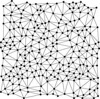
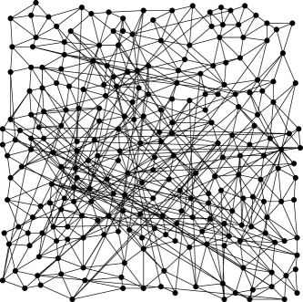
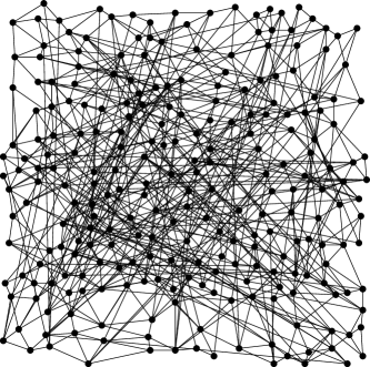
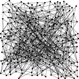
Figure 24: The Delaunay geographical network (DLN) for several numbers of rewirings: original (a) and after 60 (b), 120 (c) and 200 (d) rewirings.

A total of three sets of $300$ realization of each reference model (BA, ER and GN) were then generated. The networks for each set were designed to have average vertex degrees near the experimental value. The model and experimental networks were characterized in terms of the following measurements: straightness $\mathit{st}$, average vertex degree $\langle k\rangle$, Pearson correlation coefficient of vertex degrees $r$, average clustering coefficient $\widetilde{C}$, average shortest path length $\ell$, central point dominance $\mathit{CPD}$, average hierarchical degree of second level $\langle k_{2}(i)\rangle$, average hierarchical clustering coefficient of second level $\langle C_{2}(i)\rangle$ and average hierarchical divergence ratio of the third level $\langle\mathit{dv}_{3}(i)\rangle$.

In order to provide a general and representative view of the effect of these measurements in the classification of real networks by using the methodology involving the canonical analysis followed by Bayesian decision, we considered the following combinations of measurements:

1. $\{\ell,st\}$,

2. $\{\langle k\rangle,\widetilde{C},\ell\}$,

3. $\{\langle k_{2}(i)\rangle,\langle C_{2}(i)\rangle,\langle\mathit{dv}_{3}(i)\rangle\}$,

4. $\{st,r,\mathit{CPD}\}$,

5. $\{\langle k\rangle,\widetilde{C},\ell,st,r,\mathit{CPD}\}$,

6. $\{\langle k\rangle,\widetilde{C},\ell,\langle k_{2}(i)\rangle,\langle C_{2}(i)\rangle,\langle\mathit{dv}_{3}(i)\rangle\}$,

7. $\{st,r,\mathit{CPD},\langle k_{2}(i)\rangle,\langle C_{2}(i)\rangle,\langle\mathit{dv}_{3}(i)\rangle\}$,

8. all measurements.

The combination (i) was the only one that did not require canonical analysis. Table 4 shows the results, i.e. the theoretical model and respective average vertex degree which have been associated to each experimental network by the classification procedure, obtained for each of these configurations. More specifically, each experimental network was classified as having the same category as the theoretical model defining the decision region in the canonical projection space where the feature vector of the experimental data was mapped.

Table 4: The classes assigned to the real networks by considering each combination of measurements. The classes in bold mean wrong identified model and, in italic style, wrong average vertex degree. The $*$ symbol represents an identified class well away from all theoretical models (see, for instance, Figure 26(c)).

Experimental	Expected	Identified networks for the following combinations:
Network	Network	(i)	(ii)	(iii)	(iv)	(v)	(vi)	(vii)	(viii)
US Airlines Trans-
portation Network	BA/GN	BA	GN*	GN*	BA	BA*	BA*	GN*	BA*
(USATN)	$\langle k\rangle=12.8$	$\mathit{\langle k\rangle=10.0}$	$\mathit{\langle k\rangle=10.0}$	$\langle k\rangle=12.8$	$\mathit{\langle k\rangle=10.0}$	$\mathit{\langle k\rangle=10.0}$	$\mathit{\langle k\rangle=10.0}$	$\mathit{\langle k\rangle=14.0}$	$\langle k\rangle=12.0$
$\langle k\rangle=12.8$
Autonomous
System (AS)	BA	BA	GN	BA	BA	GN	GN	BA	GN
$\langle k\rangle=3.59$	$\langle k\rangle=3.59$	$\mathit{\langle k\rangle=6.0}$	$\langle k\rangle=3.59$	$\mathit{\langle k\rangle=6.0}$	$\langle k\rangle=4.0$	$\langle k\rangle=3.59$	$\langle k\rangle=3.59$	$\mathit{\langle k\rangle=6.0}$	$\langle k\rangle=3.59$
Transcriptional Regu-
lation Network of	BA	BA	GN	GN	BA	ER	ER	GN	ER
the E. coli (TRNE)	$\langle k\rangle=2.45$	$\langle k\rangle=2.0$	$\langle k\rangle=2.45$	$\mathit{\langle k\rangle=4.0}$	$\mathit{\langle k\rangle=4.0}$	$\langle k\rangle=2.45$	$\langle k\rangle=2.45$	$\langle k\rangle=2.45$	$\langle k\rangle=2.45$
$\langle k\rangle=2.45$
Protein-Protein
Interaction Network
of the Saccharomyces	BA	ER	GN	GN	ER	GN	GN	ER	GN
Cerevisiae (PPIN)	$\langle k\rangle=3.03$	$\mathit{\langle k\rangle=2.0}$	$\langle k\rangle=3.03$	$\mathit{\langle k\rangle=2.0}$	$\mathit{\langle k\rangle=2.0}$	$\langle k\rangle=3.03$	$\langle k\rangle=3.03$	$\mathit{\langle k\rangle=2.0}$	$\langle k\rangle=3.03$
$\langle k\rangle=3.03$
Delaunay
Network (DLN)	GN	GN	GN	GN	GN	GN	GN	GN	GN
$\langle k\rangle=6.0$	$\langle k\rangle=6.0$	$\mathit{\langle k\rangle=4.0}$	$\mathit{\langle k\rangle=4.0}$	$\langle k\rangle=6.0$	$\mathit{\langle k\rangle=4.0}$	$\mathit{\langle k\rangle=4.0}$	$\langle k\rangle=6.0$	$\langle k\rangle=6.0$	$\langle k\rangle=6.0$

A number of interesting facts can be inferred from Table 4. To begin with, the compatibility between the type of network model expected and obtained for each of the experimental networks varies considerably for each case. The best compatibility was obtained for the DLN, i.e. the identified model was compatible with the expected type (geographical) for all considered combinations of measurements. Compatible average vertex degrees have also been obtained for cases (iii), (vi)-(viii). Figure 25 illustrates the location of this network in the scatterplot defined by the canonical projection of the combination of all measurements. In this figure, which also shows the separating frontiers of the decision regions, the experimental network DLN (represented as $\diamond$) resulted closer to GN with average vertex degree of $6$. PPIN implied the highest number of incompatible classifications which, instead of being identified as a scale-free network (as expected [174]), was understood as GN except for the cases $\{\ell,st\}$ and $\{st,r,\mathit{CPD}\}$. A similar situation was verified regarding the average vertex degrees. Figure 26(c) and (d) show the resulting position of this network within the scatterplots obtained by canonical projection of the combination of all measurements (c) and all except those hierarchical (d). Note the good agreement between the resulting categories obtained for these two cases. In both cases, the PPIN resulted very close to the GN with average vertex degree of $3.03$.

Figure 25: Separating frontiers between the decision regions in the scatterplots obtained by canonical analysis for the DLN. The separating frontiers were obtained by Bayesian decision theory. Note the trajectory defined by the mapping of the progressively rewired versions of the original DLN network, extending from the GN towards the ER region with $\langle k\rangle=6$.

Figure 26: Examples of classification by canonical variable analysis and Bayesian decision theory: (a) US Airlines Transportation Network (USATN); (b) the Transcriptional Regulation Network of the E. coli (TRNE); and (c) the Protein-Protein Interaction Network of the Saccharomyces Cerevisiae (PPIN), considering all measurements; (d) the same protein network as in (c) but excluding the hierarchical measurements. Note the presence of the separating frontiers between the decision regions in the scatterplots. The arrows indicate the experimental networks.

A particularly interesting result has been obtained for the USATN, which tended to appear well away from all theoretical groups in most cases, as illustrated in the scatterplot shown in Figure 26(a) with respect to the case $\{\langle k\rangle,\widetilde{C},\ell\}$. Intermediate results were obtained for the other networks. For instance, TRNE has been classified as expected (i.e. as a BA network) in $2$ cases, identified as an ER in only one case and as a GN in $5$ cases. Figure 26(b) shows the position of this network in the scatterplot defined for all measurements. Note that TRNE appears almost in the middle of the ER and GN types for average vertex degree of $2.45$.

It is also possible to use hierarchical clustering algorithms (e.g. [40, 39, 158]) in order obtain additional information about the relationship between the analyzed networks. Figure 27 shows the dendrogram obtained for the situation depicted in Figure 26(c) by using Ward’s aglomerative method. In this method the networks, inititally treated as individual clusters, are progressively merged in order to guarantee minimal dispersion inside each cluster. The linkage distance is shown along the $y-$axis, indicating the point where the clusters are merged (the sooner two clusters are merged, the most similar they are). The similarity between the cases belonging to each of the three types of networks is reflected by the fact that three respective main branches are obtained in the dendrogram in Figure 27. The GN cluster incorporates the experimental protein-protein network, to which it is most closely related by the measurements. Note that the GN group, including the protein-protein network, is significantly different from the ER and BA models at the right-hand side of the figure, as indicated by the high linkage distance at which these two groups (i.e. the GN and ER/BA) are merged.

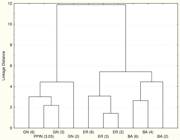
Figure 27: Dendrogram obtained for the protein-protein interaction network considering all measurements except those hierarchical. Note that the BA, ER and GN networks resulted in well-separated branches, while the protein-protein network was included into the latter group.

The results discussed above illustrate the classification procedure and its potential for identifying the category of networks of unknown nature. The fact that the assigned category sometimes varies according to the choice of measurements suggests the presence of specific topological features in some experimental networks which are not fully compatible with any of the assumed theoretical models. Indeed, the consideration of more measurements can, in principle, provide a more comprehensive subclassification of the networks. Such a possibility is particularly important in the case of scale-free networks, which are known to involve subtypes [24]. For instance, TRNE has been identified in our experiments as having BA type while considering two measurements (i.e. $\{st,\ell\}$), but was understood as a GN model by considering three measurements (i.e. $\{\langle k\rangle,\widetilde{C},\ell\}$) and as ER when we considered six measurements (i.e. $\{\langle k\rangle,\widetilde{C},\ell,st,r,\mathit{CPD}\}$).

It should be always kept in mind that the consideration of an excessive number of measurements may ultimately compromise the quality of the classification. Methodologies such as the canonical analysis followed by Bayesian classification can be used to identify the features which contribute the most for the correct classifications. This can be done by considering the measurements which contribute more intensely for the canonical projections providing the largest number of correct classifications. A simpler methodology involves the application of the principal component analysis to remove the redundancies between the measurements. In the case of a reduced number of measurements it is also possible to consider all the respective combinations and evaluate which of them yields the best classifications. Another interesting possibility for investigating complex network connectivity is to consider outliers analysis (e.g. [166]). The reader interested in additional information on multivariate statistics and feature selection is referred to the specialized literature (e.g., [40, 39, 168, 167]) for more in-depth discussion and coverage.

19 Concluding Remarks

Measurements of the connectivity and topology of complex networks are essential for the characterization, analysis, classification, modeling and validation of complex networks. Although initially limited to simple features such as vertex degree, clustering coefficient and shortest path length, several novel, powerful measurements have been proposed. We hope it has been made clear that the several available measurements often provide complementary characterization of distinct connectivity properties of the structures under analysis. It is only by becoming familiar with such measurements that one can expect to identify proper sets of features to be used for the characterization of complex networks. The current survey has been organized to provide a comprehensive coverage of not only the most traditional measurements but also complementary alternatives which, though not so frequently used, can provide valuable resources for characterizing specific topological properties of complex networks. Special attention was also given to the application of measurements in community finding algorithms, an important issue in complex network research.

In addition to presenting such measurements according to coherent categories, we also addressed issues such as visualization, in terms of trajectories defined by measurements, of complex network growth. As illustrated by the results presented, which considered several important theoretical network models, such trajectories clearly reflect, in graphical terms, important tendencies exhibited by different network categories as their average degree is increased. Another important point to be kept in mind in network measurements is correlations. While high correlation between a pair of measurements indicates that they are largely redundant, our results show that the own correlation values vary from one network model to another, providing further useful information for network characterization. Another important property of a specific measurement is its sensitivity to small perturbations in the network, such as the inclusion or removal of edges or vertices. We illustrated that different measurements can behave very differently with respect to such induced changes. Because one of the most challenging issues related to network categorization regards the choice of the features to be taken into account, we provided a self-contained discussion about how multivariate statistics concepts and methods can be applied for that aim. More specifically, we showed how high dimensional measurement spaces can be effectively projected, by using principal component analysis, into lower-dimensional spaces favoring visualization and application of computationally intensive measurements. We also described how two useful methods, namely canonical analysis and Bayesian decision theory, can be combined to provide the means for semi-automated identification of the effective linear combinations of measurements, in the sense of allowing good discrimination between network categories. The potential of such multivariate methodologies was illustrated for theoretical models and experimental networks. The results clearly suggested that considering a comprehensive set of measurements can provide more complete characterization of the topological properties of the networks to the point of requiring a revision of the traditional classification of experimental networks into subclasses or new models.

All in all, this survey provides for the first time an integrated presentation and discussion of a comprehensive set of measurements previously covered in separated works. In addition, it addresses important issues related to application of these measurements for characterization and classification of networks, including dynamical representations in terms of trajectories, redundancy between measurements as quantified by correlations, perturbation effects and a powerful multivariate framework for classification of networks of unknown category. The systematic application of such concepts and tools is poised to yield a wealthy of new results in the study of complex networks.

References

- [1] P. J. Flory. Molecular size distribution in three-dimensional polymers. I. Gelation. Journal of the American Chemical Society, 63:3083–3090, 1941.
- [2] A. Rapoport. Nets with distance bias. Bulletin of Mathematical Biophysics, 13:85–91, 1951.
- [3] A. Rapoport. Spread of information through a population with socio-structural bias: I. Assumption of transitivity. Bulletin of Mathematical Biophysics, 15:523–533, 1953.
- [4] A. Rapoport. Contribution to the theory of random and biased nets. Bulletin of Mathematical Biophysics, 19:257–277, 1957.
- [5] P. Erdős and A. Rényi. On random graphs. Publicationes Mathematicae, 6:290–297, 1959.
- [6] P. Erdős and A. Rényi. On the evolution of random graphs. Publ. Math. Inst. Hungar. Acad. Sci, 5:17–61, 1960.
- [7] P. Erdős and A. Rényi. On the strenght of connectedness of a random graph. Acta Mathematica Scientia Hungary, 12:261–267, 1961.
- [8] D. J. Watts and S. H. Strogatz. Collective dynamics of small-world networks. Nature, 393(6684):440–442, 1998.
- [9] A.-L. Barabási and R. Albert. Emergence of scaling in random networks. Science, 286:509–512, 1997.
- [10] M. Girvan and M. E. J. Newman. Community structure in social and biological networks. Proceedings of the National Academy of Science USA, 99(12):7821–7826, 2002.
- [11] B. Bollobás. Modern Graph Theory. Graduate Texts in Mathematics, Springer-Verlag, New York, 1998.
- [12] D. B. West. Introduction to Graph Theory. Prentice Hall, 2001.
- [13] J. P. Scott. Social Network Analysis: A Handbook. Sage Publications, 2000.
- [14] M. E. J. Newman and J. Park. Why social networks are different from other types of networks. Physical Review E, 68(036122), 2003.
- [15] A.-L. Barabási and Z. N. Oltvai. Network biology: Understanding the cells functional organization. Nature, 5:101–113, 2004.
- [16] S. Bornholdt and H. G. Schuste, editors. Handbook of Graphs and Networks: From the Genome to the Internet. Wiley-VCH, 2003.
- [17] L. A. N. Amaral and J. M. Ottino. Complex networks. European Physical Journal B, 38:147–162, 2004.
- [18] M. Faloutsos, P. Faloutsos, and C. Faloutsos. On power-law relationships of the internet topology. Computer Communication Review, 29(4):251–262, 1999.
- [19] R. Albert, H. Jeong, and A.-L. Barabási. Diameter of the world wide web. Nature, 401:130–131, 1999.
- [20] A.-L. Barabási, R. Albert, and H. Jeong. Scale-free characteristics of random networks: the topology of the world wide web. Physica A, 281:69–77, 2000.
- [21] R. Albert and A.-L. Barabási. Statistical mechanics of complex networks. Reviews of Modern Physics, 74:48–98, 2002.
- [22] S. N. Dorogovtsev and J. F. F. Mendes. Evolution of networks. Advances in Physics, 51:1079–1187, 2002.
- [23] M. E. J. Newman. Structure and function of complex networks. SIAM Review, 45(2):167–256, 2003.
- [24] S. Boccaletti, V. Latora, Y. Moreno, M. Chaves, and D.-U. Hwang. Complex networks: structure and dynamics. Physics Reports, 424:175–308, 2006.
- [25] A.-L. Barabási and E. Bonabeau. Scale-free networks. Scientific American, 288:60–69, 2003.
- [26] B. Hayes. Graph Theory in Practice: Part I. American Scientist, 88(1):9–13, 2000.
- [27] B. Hayes. Graph theory in practice: Part II. American Scientist, 88(2):104–109, 2000.
- [28] B. Bollobás. Random graphs. Academic Press, Inc., 1985.
- [29] S. Wasserman and K. Faust. Social Network Analysis. Cambridge University Press, 1994.
- [30] A.-L. Barabási. Linked: How Everything Is Connected to Everything Else and What It Means. Plume, 2002.
- [31] S. N. Dorogovtsev and J. F. F. Mendes. Evolution of Networks – From Biological Nets to the Internet and WWW. Oxford University Press, 2003.
- [32] M. E. J. Newman, A.-L. Barábasi, and D. J. Watts, editors. The Structure and Dynamics of Networks. Princeton University Press, 2006.
- [33] D. Stauffer and A. Aharony. Introduction to Percolation Theory. Taylor and Francis, 1994.
- [34] A. Bunde and S. Havlin. Fractals and Disordered Systems. Springer, 1996.
- [35] A. Bunde and S. Havlin. Fractals in Science. Springer, 1995.
- [36] N. Boccara. Modeling Complex Systems. Springer-Verlag New York, 2004.
- [37] Y. Bar-Yam. Dynamics of Complex Systems. Perseus Books, 1992.
- [38] S. Strogatz. Sync: The Emerging Science of Spontaneous Order. Hyperion, 2003.
- [39] L. da F. Costa and R. M. Cesar Jr. Shape Analysis and Classification: Theory and Practice. CRC Press, 2001.
- [40] R. O. Duda, P. E. Hart, and D. G. Stork. Pattern Classification. John Wiley & Sons, Inc., 2001.
- [41] E. Ziv, R. Koytcheff, M. Middendorf, and C. Wiggins. Systematic identification of statistically significant network measures. Physical Review E, 71:016110, 2005.
- [42] M. Barthélemy, A. Barrat, R. Pastor-Satorras, and A. Vespignani. Characterization and modeling of weighted networks. Physica A, 346:34–43, 2005.
- [43] D. J. Watts. Small worlds : the dynamics of networks between order and randomness. Princeton University Press, 1999.
- [44] D. J. Watts. Six Degrees. The Science of a Connected Age. W.W. Norton & Company, 2003.
- [45] S. Milgran. The small world problem. Psychology Today, 1(1):60–67, 1967.
- [46] R. Monasson. Diffusion, localization and dispersion relations on “small-world” lattices. European Physical Journal B, 12(555), 1999.
- [47] M. E. J. Newman and D. J. Watts. Renormalization group analysis of the small-world network model. Physical Review Letters A, 263:341–346, 1999.
- [48] E. A. Bender and E. R. Can. The asymptotic number of labeled graphs with given degree sequences. Journal of Combinatorial Theory, Ser. A 24:296–307, 1978.
- [49] M. Molloy and B. Reed. A critical point for random graphs with a given degree sequence. Random Structures and Algorithms, 6:161–179, 1995.
- [50] M. Molloy and B. Reed. The size of the giant component of a random graph with a given degree sequence. Probability and Computing, 7:295–305, 1998.
- [51] M. E. J. Newman. Random graphs as models of networks. In S. Bornholdt and H. G. Schuster, editors, Handbook of Graphs and Networks: From the Genome to the Internet. Wiley-VCH, 2003.
- [52] M. E. J. Newman, D. J. Watts, and S. H. Strogatz. Random graphs with arbitrary degree distributions and their applications. Proceedings of the National Academy of Science USA, 99:2566–2572, 2002.
- [53] M. E. J. Newman, S. H. Strogatz, and D. J. Watts. Random graphs with arbitrary degree distributions and their applications. Physical Review E, 64(026118), 2001.
- [54] R. Milo, N. Kashtan, S. Itzkovitz, M. E. J. Newman, and U. Alon. On the uniform generation of random graphs with prescribed degree sequences. cond-mat/0312028, 2003.
- [55] W. Aiello, F. Chung, and L. Lu. A random graph model for massive graphs. In Proceedings of the thirty-second annual ACM symposium on Theory of computing, pages 171–180, Portland, Oregon, United States, 2000. ACM Press.
- [56] F. Chung and L. Lu. The average distances in random graphs with given expected degrees. Proceedings of the National Academy of Science USA, 99:15879–15882, 2002.
- [57] R. Cohen and S. Havlin. Scale-free networks are ultrasmall. Physical Review Letters, 90(058701), 2003.
- [58] M. T. Gastner and M. E. J. Newman. The spatial structure of networks. The European Physical Journal B, 49:247, 2006.
- [59] R. Albert, I. Albert, and G. L. Nakarado. Structural vulnerability of the north american power grid. Physical Review E, 69:025103, 2004.
- [60] R. Kinney, P. Crucitti, R. Albert, and V. Latora. Modeling cascading failures in the north american power grid. European Physical Journal B, 46:101–107, 2005.
- [61] A. Barrat, M. Barthélemy, R. Pastor-Satorras, and A. Vespignani. The architecture of complex weighted networks. Proceedings of the National Academy of Science USA, 101(11):3747–3752, 2004.
- [62] R. Guimerà, S. Mossa, A. Turtschi, and L. A. N. Amaral. The worldwide air transportation network: Anomalous centrality, community structure, and cities’ global roles. Proceedings of the National Academy of Science USA, 102:7794–7799, 2005.
- [63] Y. Hayashi. A review of recent studies of geographical scale-free networks. physics/0512011, 2005.
- [64] V. Latora and M. Marchiori. Is the boston subway a small-world network? Physica A, 314:109–113, 2002.
- [65] O. Sporns. Network analysis, complexity and brain function. Complexity, 8(56–60), 2002.
- [66] M. Kaiser and C. C. Hilgetag. Spatial growth in real-time networks. Phys. Rev. E, 69:036103, 2004.
- [67] V. Latora and M. Marchiori. Efficient behavior of small-world networks. Physics Review Letters, 87:198701, 2001.
- [68] R. Guimerà, A. Díaz-Guilera, F. Vega-Redondo, A. Cabrales, and A. Arenas. Optimal network topologies for local search with congestion. Physical Review Letters, 89:248701, 2002.
- [69] V. Gol’dshtein, G. A. Koganov, and G. I. Surdutovich. Vulnerability and hierarchy of complex networks. cond-mat/0409298, 2004.
- [70] V. Latora and M. Marchiori. Vulnerability and protection of critical infrastructures. Physical Review E, 71:015103R, 2005.
- [71] M. E. J. Newman. Scientific collaboration networks: I. Network construction and fundamental results. Physical Review E, 64:016131, 2001.
- [72] J.-P. Onnela, J. Saramäki, J. Kertész, and K. Kaski. Intensity and coherence of motifs in weighted complex networks. Physical Review E, 71:065103(R), 2005.
- [73] E. Ravasz and A.-L. Barabási. Hierarchical organization in complex networks. Physical Review E, 67:026112, 2003.
- [74] S. N. Soffer and A. Vázquez. Clustering coefficient without degree correlations biases. Physical Review E, 71:057101, 2005.
- [75] H. J. Kim and J. M. Kim. Cyclic topology in complex network. Physical Review E, 72:036109, 2005.
- [76] V. Colizza, A. Flammini, M. A. Serrano, and A. Vespignani. Detecting rich-club ordering in complex networks. Nature Physics, 2:110–115, 2006.
- [77] S. Zhou and R. J. Mondragon. The rich-club phenomenon in the internet topology. Communications Letters, IEEE, 8(3):180–182, 2004.
- [78] S. N. Dorogovtsev and J. F. F. Mendes. The shortest path to complex networks. cond-mat/0404593, 2004.
- [79] S. Maslov and K. Sneppen. Specificity and stability in topology of protein networks. Science, 296(5569):910–913, 2002.
- [80] M. Bogu ná and R. Pastor-Satorras. Epidemic spreading in correlated complex networks. Physical Review E, 66:047104, 2002.
- [81] M. Bogu ná, R. Pastor-Satorras, and A. Vespignani. Statistical mechanics of complex networks. Lecture and Notes in Physics, 625(127), 2003.
- [82] R. Pastor-Satorras, A. Vazquez, and A. Vespignani. Dynamical and correlation properties of the internet. Physical Review Letters, 87(25):258701, 2001.
- [83] M. E. J. Newman. Assortative mixing in networks. Physical Review Letters, 89(20):208701, 2002.
- [84] M. Catanzaro, G. Caldarelli, and L. Pietronero. Assortative model for social networks. Physical Review E, 70:037101, 2004.
- [85] J. Park and M. E. J. Newman. The origin of degree correlations in the internet and other networks. Physical Review E, 68:026112, 2003.
- [86] J. Berg, M. Lässig, and A. Wagner. Structure and evolution of protein interaction networks: A statistical model for link dynamics and gene duplications. BMC Evolutionary Biology, 4:51, 2004.
- [87] M. Brede and S. Sinha. Assortative mixing by degree makes a network more unstable. cond-mat/0507710, 2005.
- [88] M. di Bernardo, F. Garofalo, and F. Sorrentino. Synchronization of degree correlated physical networks. cond-mat/0506236, 05.
- [89] M. di Bernardo, F. Garofalo, and F. Sorrentino. Synchronizability of degree correlated networks. To appear in International Journal of Bifurcations and Chaos, 2006.
- [90] N. Madar, T. Kalisky, R. Cohen, D. ben Avraham, and S. Havlin. Immunization and epidemic dynamics in complex networks. The European Physical Journal B, 38:269–276, 2004.
- [91] T. Zhou, Z.-Q. Fu, and B.-H. Wang. Epidemic dynamics on complex networks. Progress in Natural Science, 16:452–457, 2006.
- [92] S. Gupta, R. M. Anderson, and R. M. May. Network of sexual contacts: Implications for the pattern of spread of HIV. AIDS, 03:807–817, 1989.
- [93] M. E. J. Newman. Mixing patterns in networks. Physical Review E, 67:026126, 2003.
- [94] P. Holme, F. Liljeros, C. R. Edling, and B. J. Kim. Network bipartivity. Physical Review E, 68:056107, 2003.
- [95] E. Estrada and J. A. Rodríguez-Veláquez. Spectral measures of bipartivity in complex networks. Physical Review E, 72:046105, 2005.
- [96] F. Reif. Fundamentals of statistical and thermal physics. McGraw-Hill, 1965.
- [97] L. Brillouin. Science and Information Theory. Dover Phoenix Editions, 2004.
- [98] L. E. Reichl. A Modern Course in Statistical Physics. Wiley-Interscience, 1998.
- [99] C. E. Shannon and W. Weaver. The Mathematical Theory of communication. University of Illinois, 1963.
- [100] B. Wang, H. Tang, C. Guo, and Z. Xiu. Entropy optimization of scale-free networks robustness to random failures. cond-mat/0506725, 2005.
- [101] L. Demetrius and T. Manke. Robustness and network evolution — an entropic principle. Physica A, 346(3–4):682–696, 2004.
- [102] R. V. Solé and S. Valverde. Information theory of complex networks in: Complex networks. In E. Ben-Naim, H. Frauenfelder, and Z. Toroczkai, editors, Lecture Notes in Phyics, pages 169–190, Berlin, 2004. Springer.
- [103] K. Sneppen, A. Trusina, and M. Rosvall. Hide and seek on complex networks. Europhysics Letters, 69(5):853–859, 2005.
- [104] M. Rosvall and K. Sneppen. Networks and our limited information horizon. cond-mat/0604036, 2006.
- [105] M. Rosvall, A. Trusina, P. Minhagen, and K. Sneppen. Networks and cities: An information perspective. Physical Review Letters, 94:028701, 2005.
- [106] A. Trusina, M. Rosvall, and K. Sneppen. Information horizons in networks. Physical Review Letters, 94:238701, 2005.
- [107] M. Rosvall, A. Grönlund, P. Minnhagen, and K. Sneppen. Searchability of networks. Physical Review E, 72:046117, 2005.
- [108] L. C. Freeman. A set of measures of centrality based on betweenness. Sociometry, 40:35–41, 1977.
- [109] A. Arenas, A. Cabrales, A. Díaz-Guilera, R. Guimerà, and F. Vega-Redondo. Search and congestion in complex networks. In Statistical Mechanics of Complex Networks, volume 625 of Lecture Notes in Physics. Springer, 2003.
- [110] M. E. J. Newman. A measure of betweenness centrality based on random walks. Social Networks, 27:39–54, 2005.
- [111] D. Koschützki, K. A. Lehmann, L. Peeters, S. Richter, D. Tenfelde-Podehl, and O. Zlotowski. Centrality indices. Lecture Notes in Computer Science, 3418, 2005.
- [112] I. J. Farkas, I. Derenyi, A.-L. Barabási, and T. Vicsek. Spectra of “real-world” graphs: beyond the semicircle law. Physical Review E, 64:026704, 2001.
- [113] K.-I. Goh, B. Kahng, and D. Kim. Spectra and eigenvectors of scale-free networks. Physical Review E, 64:051903, 2001.
- [114] V. Rosato and F. Tiriticco. Growth mechanisms of the AS-level internet network. Europhysics Letters, 66(4):471–477, 2004.
- [115] M. L. Mehta. Random Matrices. Academic Press, 1991.
- [116] A. J. Seary and W. D. Richards. Spectral methods for analyzing and visualizing networks: an introduction. In Dynamic Social Network Modeling and Analysis, pages 209–228. National Academy Press, 2003.
- [117] A. Arenas, L. Danon, A. Díaz-Guilera, P. M. Gleiser, and R. Guimerà. Community analysis in social networks. European Physical Journal B, 38:373–380, 2004.
- [118] P. M. Gleiser and L. Danon. Community structure in jazz. Advances in complex systems, 6(4), 2003.
- [119] R. Guimerà and L. A. N. Amaral. Functional cartography of complex metabolic networks. Nature, 433:895–900, 2005.
- [120] F. Radicchi, C. Castellano, F. Cecconi, V. Loreto, and D. Parisi. Defining and identifying communities in networks. Proceedings of the National Academy of Science USA, 101(9):2658–2663, 2004.
- [121] J. Reichardt and S. Bornholdt. Statistical mechanics of community detection. cond-mat/0603718, 2006.
- [122] J. Reichardt and S. Bornholdt. When are networks truly modular? cond-mat/0606220, 2006.
- [123] J. Reichardt and S. Bornholdt. Detecting fuzzy community structures in complex networks with a potts model. Physical Review Letters, 93(218701), 2004.
- [124] M. E. J. Newman and M. Girvan. Finding and evaluating community structure in networks. Physical Review E, 69:026113, 2004.
- [125] G. Schlosser and G. P. Wagner. Modularity in Development and Evolution. University of Chicago Press, 2004.
- [126] E. Ziv, M. Middendorf, and C. H. Wiggins. Information-theoretic approach to network modularity. Physical Review E, 71:046117, 2005.
- [127] M. E. J. Newman. Detecting community structure in networks. The European Physical Journal B, 38:321–330, 2004.
- [128] L. Danon, J. Duch, A. Arenas, and A. Díaz-Guilera. Comparing community structure identification. Journal of Statistical Mechanics: Theory and Experiment, page P09008, 2005.
- [129] A. J. Seary and W. D. Richards. Partitioning networks by eigenvectors. In Proceedings of the International Conference on Social Networks, volume 1, 1995.
- [130] M. E. J. Newman. Finding community structure in networks using the eigenvectors of matrices. physics/0605087, 2006.
- [131] M Fiedler. Algebraic connectivity of graphs. Czechoslovak Mathematical Journal, 23(298):298–305, 1973.
- [132] A. Pothen, H. Simon, and KP Liou. Partitioning sparse matrices with eigenvectors of graphs. SIAM Journal on Matrix Analysis and Applications, 11(430):430–452, 1990.
- [133] A. Capocci, V. D. P. Servedio, G. Caldarelli, and F. Colaiori. Detecting communities in large networks. Physica A, 352:669–676, 2005.
- [134] M. E. J. Newman. Modularity and community structure in networks. Proceedings of the National Academy of Science USA, 103:8577–8582, 2006.
- [135] J. R. Tyler, D. M. Wilkinson, and B. A. Huberman. Email as spectroscopy: Automated discovery of community structure within organizations. In M. Huysman, editor, In Proceedings of the First International Conference on Communities and Technologies, 2003.
- [136] L. da F. Costa. L-percolations of complex networks. Phys. Rev. E, 70:056106, 2004.
- [137] M. R. Anderberg. Cluster analysis for applications. Academic Press, 1973.
- [138] A. K. Jain and R. C. Dubes. Algorithms for clustering data. Prentice Hall, 1988.
- [139] H. C. Romesburg. Cluster analysis for researchers. Robert E. Krieger, 1990.
- [140] J. Hopcroft, O. Khan, B. Kulis, and B. Selman. Tracking evolving communities in large linked networks. Proceedings of the National Academy of Science USA, 101:5249–5253, 2004.
- [141] A. Clauset, M. E. J. Newman, and C. Moore. Finding community structure in very large networks. Physical Review E, 70:066111, 2004.
- [142] L. Danon, A. Díaz-Guilera, and A. Arenas. Effect of size heterogeneity on community identification in complex networks. physics/0601144, 2006.
- [143] J. Duch and A. Arenas. Community detection in complex networks using extremal optimization. Physical Review E, 72:027104, 2005.
- [144] M. E. J. Newman. Fast algorithm for detecting community structure in networks. Physical Review E, 69, 2004.
- [145] J.P. Bagrow and E. M. Bollt. A local method for detecting communities. Physical Review E, 72:046108, 2005.
- [146] A. Clauset. Finding local community structure in networks. Physical Review E, 72:026132, 2005.
- [147] S. S. Shen-Orr, R. Milo, S. Mangan, and U. Alon. Network motifs in the transcriptional regulation network of Escherichia Coli. Nature Genetics, 31:64–68, 2002.
- [148] R. Milo, S. Shen-Orr, S. Itzkovitz, N. Kashtan, D. Chklovskii, and U. Alon. Network motifs: simple building blocks of complex networks. Science, 298:824–827, 2002.
- [149] M. Middendorf, E. Ziv, and C. H. Wiggins. Inferring network mechanisms: the drosophila melanogaster protein interaction network. Proceedings of the National Academy of Sciences, 102(9):3192–3197, 2005.
- [150] R. Milo, S. Itzkovitz, N. Kashtan, R. Levitt, S. Shen-Orr, I. Ayzenshtat, M. Sheffer, and U. Alon. Superfamilies of evolved and designed networks. Science, 303(5663):1538–1542, 2004.
- [151] E. Estrada and J. A. Rodríguez-Veláquez. Subgraphs centrality in complex networks. Physical Review E, 71:056103, 2005.
- [152] L. Vincent. Graphs and mathematical morphology. Signal Processing, 16(4):365–388, 1989.
- [153] E. R. Dougherty and R. A. Lotufo. Hands-on Morphological Image Processing. SPIE Press, 2003.
- [154] H. Heijmans, P. Nacken, A. Toet, and L. Vincent. Graph morphology. Journal of Visual Communication and Image Representation, 3(1):24–38, 1990.
- [155] M. P. Viana and L. da F. Costa. The dynamics of hierarchical evolution of complex networks. cond-mat/0504346, 2005.
- [156] L. da F. Costa. The hierarchical backbone of complex networks. Physical Review Letters, 93(098702), 2004.
- [157] L. da F. Costa and L. E. C. da Rocha. A generalized approach to complex networks. Eur. Phys. J. B, 50, 2006.
- [158] L. da F. Costa and F. N. Silva. Hierarchical characterization of complex networks. J. Stat. Phys. (accepted), 2004. cond-mat/0412761.
- [159] C. Song, S. Havlin, and H. A. Makse. Self-similarity of complex networks. Nature, 433(27):392–395, 2005.
- [160] B. Machta and J. Machta. Parallel dynamics and computational complexity of network growth models. Physical Review E, 71:026704, 2005.
- [161] B. Codenotti and M. Leoncini. Introduction to Parallel Processing. Addison-Wesley, 1993.
- [162] H. Meyer-Ortmanns. Functional complexity measure for networks. cond-mat/0311109, 2003.
- [163] J. C. Claussen. Offdiagonal complexity: A computationally quick complexity measure for graphs and networks. q-bio.MN/0410024, 2004.
- [164] D. Garlaschelli and M. I. Loffredo. Patterns of link reciprocity in directed networks. Physical Review Letters, 93(26):268701, 2004.
- [165] M. Kaiser and C. C. Hilgetag. Edge vulnerability in neural and metabolic networks. Biological Cybernetics, 90:311–317, 2004.
- [166] L. da F. Costa, M. Kaiser, and C. Hilgetag. Beyond the average: detecting global singular nodes from local features in complex networks. physics/0607272, 2006.
- [167] K. Fukunaga. Introduction to Statistical Pattern Recognition. Academic Press, 1990.
- [168] G. J. McLachlan. Discriminant Analysis and Statistical Pattern Recognition. Wiley, 2004.
- [169] J. F. Hair, R. E. Anderson, R. L. Tatham, and W. C. Black. Multivariate Data Analysis. Prentice-Hall Int. Inc., 1998.
- [170] R. A. Johnson and D. W. Wichern. Applied Multivariate Statistical Analysis. Prentice Hall, fifth edition, 2002.
- [171] P. R. R. Prado, F. F. Franco, M. H. Manfrin, and L. da F. Costa. An easy and fast way to analyse morphometric characters. In R. Mondaini, editor, Proceedings of the Third Brazilian Symposium of Mathematical and Computacional Biology I, pages 329–340, Rio de Janeiro, 2004. E-papers publishing.
- [172] V. Batagelj and A. Mrvar. Pajek datasets. University of Ljubljana, Slovenia, http://vlado.fmf.uni-lj.si/pub/networks/data, 2006.
- [173] R. Guimerà and L. A. N. Amaral. Modeling the world-wide airport network. European Physical Journal B, 38:381–385, 2004.
- [174] H. Jeong, S. P. Mason, A.-L. Barabási, and Z. N. Oltvai. Lethality and centrality in protein networks. Nature, 411(6833):41–42, 2001.
- [175] S. H. Yook, H. Jeong, and A.-L. Barabási. Modeling the internet’s large-scale topology. Proceedings of the National Academy of Science USA, 99:13382–13386, 2002.
- [176] D. Stoyan, W. S. Kendall, and J. Mecke. Stochastic Geometry and Its Applications. John Wiley and Sons, 1996.