Mode-coupling theory for multiple-time correlation functions of tagged particle densities and dynamical filters designed for glassy systems

Abstract

The theoretical framework for higher-order correlation functions involving multiple times and multiple points in a classical, many-body system developed by Van Zon and Schofield [Phys. Rev. E 65, 011106 (2002)] is extended here to include tagged particle densities. Such densities have found an intriguing application as proposed measures of dynamical heterogeneities in structural glasses. The theoretical formalism is based upon projection operator techniques which are used to isolate the slow time evolution of dynamical variables by expanding the slowly-evolving component of arbitrary variables in an infinite basis composed of the products of slow variables of the system. The resulting formally exact mode-coupling expressions for multiple-point and multiple-time correlation functions are made tractable by applying the so-called $N$-ordering method. This theory is used to derive for moderate densities the leading mode coupling expressions for indicators of relaxation type and domain relaxation, which use dynamical filters that lead to multiple-time correlations of a tagged particle density. The mode coupling expressions for higher order correlation functions are also succesfully tested against simulations of a hard sphere fluid at relatively low density.

I Introduction

A complete understanding of the physical processes underlying the transition between the high-temperature exponential relaxation of density fluctuations of a fluid and the non-exponential relaxational profiles observed at lower temperatures, especially near the glass transition, remains elusive. A number of interesting features have been noted in dense, supercooled systems from computer simulation studiesKobetal97 ; YamamotoOnuki98 ; YamamotoOnuki98b ; DoliwaHeuer98 ; Kob99 ; YamamotoOnuki99 ; SjodinSjolander78 as well as multi-dimensional NMRBoehmeretal96 ; Trachtetal98 and video microscopy experimentsMarcusetal99 ; Weeksetal00 that appear to be related to this cross-over from simple exponential to multi or stretched exponential relaxation: One typical feature of such systems is the appearance of heterogeneously-distributed regions of the fluid which differ dramatically in their mobility and local density. While fluid motions are relatively unrestricted in regions of low density, structural rearrangements in regions of high local density at a given time have been observed to occur through relatively rapid, collective string-like motionsKobetal97 . Furthermore, regions which at one time were of relatively low density and in which particle motions were primarily fluid-like can become locally-dense and immobile.

It is well-known that a variety of different mechanisms are consistent with non-exponential relaxation and that this relaxation is somehow related to the heterogeneous nature of the dense fluid. In one possible scenario of non-exponential relaxation, fluctuations of local density relax in the same intrinsically non-exponential way, where the cooperative motion of particles depends strongly on the local environment and is correlated over a long time period or “history”. Another possible mechanism is that each region of the fluid rearranges in a less strongly-correlated fashion but with different rates, so that the observed non-exponentiality is a consequence of the superposition of different exponential relaxation processes. Of course neither scenario may apply over all time scales and the mechanism may shift from one that is primarily homogeneous to one that is primarily heterogeneous. It is equally possible that one type of relaxation may not even predominate over another.

In order to distinguish between these scenarios it is helpful to construct quantitative measures which unambiguously signal the presence of a specific mechanism. Such constructions can be based on filtersHeuer97 ; HeuerOkun97 ; DoliwaHeuer98 ; DoliwaHeuer99 that select out sub-ensembles of particles to have specific dynamical properties over a sampling period. A simple example of such a filter is one that selects out individual particles that move either more or less than a critical distance over a fixed period of time. One can then examine time correlations within these sub-ensembles to gain new insight into detailed features of the dynamics. When time-filters are utilized in this fashion, time correlation functions of particles contained in the sub-ensemble necessarily involve multiple-time intervals. Filters based on single-particle properties then can be expressed as multiple-time correlation functions of tagged particle densities.

Given this interesting application of multiple-time correlation functions, the need for a theory that enables one to calculate such quantities from first principles is clear. In Ref. VanZonSchofield02a, such a theory was developed based on mode-coupling theory for multiple-time correlation functions of collective densities (i.e., particle number, momentum and energy densities). The theory was tested successfully on a hard sphere gas at moderate densities in the hydrodynamic limit where the relevance of mode-coupling theory is well-established. In this article, the theory is extended to include multiple-time correlation functions of arbitrary type, encompassing correlation functions involving only tagged densities, only collective densities as well as any combination of the two types.

The paper is organized as follows: The mode-coupling formalism of multiple-time correlation functions is introduced in Sec. II based on projection operator methods, and equations describing the evolution of multiple-point densities of arbitrary type are obtained. These equations are manipulated to yield expressions for correlation functions of multiple-time intervals that are local in all time arguments. In Sec. III, a systematic method of determining what types of contributions are the most significant for a particular multiple-time interval correlation function of tagged particle densities is introduced and the leading-order expressions for two and three-time interval correlations of a tagged particle density are presented. In Sec. IV, specific applications of multiple-time correlation functions of tagged particle densities are examined. In particular, direct measures of relaxation type and of the rate at which solid-like domains become fluidized are analyzed and leading order mode-coupling expressions for these measures are obtained. Sec. IV concludes with a numerical comparison of the leading order theoretical predictions with direct simulation results for a low density, hard sphere system in the hydrodynamic limit and Sec. V contains a summary.

II Mode-coupling formalism

II.1 Slow variables

The basic assumption of mode-coupling theory is that the long time behavior of all time correlations functions can be completely expressed in terms of the evolution of a set of slow modes of the system. Although the theory doesn’t specify the identity of the slow modes, physical arguments can often serve as a guide to define a finite set of variables that serve as a dynamical basis for the long time evolution. For example, since the particle number, the momentum and the total energy of a fluid of structureless particles are constants of motion, a minimal basis set for the slow evolution of the system must include the long wavelength modes of densities of these quantities.

Once the slow basis set has been determined, the slow component of an arbitrary dynamical quantity can be extracted by finding the projection of the variable onto the subspace spanned by the set of slow variables. Similarly, projecting the variable onto the complement of this subspace should yield a fast quantity.

Projection operators are linear operators, and hence only the linear dependence of a dynamical variable on the slow variables can be projected out by such a procedure. In general, however, one expects the time dependence of most dynamical variables to be a non-linear function of the slow variables. This non-linearity can be incorporated into the theory by constructing the slow subspace to include the space spanned by all powers of the slow variables. In this way an analytic dependence of the slowly-evolving component of a dynamical variable on the slow variables can be described. The basis of the slow subspace is referred to as the multi-linear basis.

Consider an equilibrium system composed of $N$ particles that is described by a translationally invariant Hamiltonian $\mathcal{H}$. The time evolution of any quantity (phase space function) $C$ is given by

$$\dot{C}(t)={\cal L}C(t),$$ (1)

with ${\cal L}$ the Liouvillian operator, which is the Poisson bracket with the Hamiltonian.

To describe the slow evolution of dynamical variables within the projection operator formalism, the slow variables of the system are taken together in a single vector $B$. As mentioned above, for a structureless fluid, these are typically the number density, the momentum density and the energy density:

$$B(\mathbf{r},t)=\left(\begin{array}[]{c}N(\mathbf{r},t)\\ \mathbf{P}(\mathbf{r},t)\\ E(\mathbf{r},t)\end{array}\right)=\left(\begin{array}[]{c}\displaystyle\sum_{n=1}^{N}\delta(\mathbf{r}-\mathbf{r}_{n}(t))\\ \displaystyle\sum_{n=1}^{N}\mathbf{p}_{n}(t)\delta(\mathbf{r}-\mathbf{r}_{n}(t))\\ \displaystyle\sum_{n=1}^{N}e_{n}(t)\delta(\mathbf{r}-\mathbf{r}_{n}(t))\end{array}\right).$$

Here, $\mathbf{r}_{n}(t)$ is the position of particle $n$ at time $t$, $\mathbf{p}_{n}(t)$ is its momentum and $e_{n}(t)$ its energy (kinetic and potential). It will be convenient to work in Fourier space:

$$B(\mathbf{k},t) = \sum_{n=1}^{N}e^{i\mathbf{k}\cdot\mathbf{r}_{n}(t)}b_{n}(t),$$ (2)

where $b_{n}(t)=(1,\mathbf{p}_{n}(t),e_{n}(t))$.

Since the goal of the mode-coupling theory outlined here is to describe the time correlation functions of single particles, slow tagged particle densities must be included, i.e.,

$$N_{1}(\mathbf{r},t) = \delta(\mathbf{r}-\mathbf{r}_{1}(t)),$$

where particle $1$ is the tagged particle. In the Fourier representation, the tagged particle number density is simply

$$N_{1}(\mathbf{k})=e^{i\mathbf{k}\cdot\mathbf{r}_{1}(t)}.$$ (3)

The tagged particle density is taken together with $B(\mathbf{k})$ into a larger vector $A(\mathbf{k})$. Henceforth, components of $A$ will be denoted with a superscript $s$ when referring to single particle densities (which have no summation over particles in their definition) and with a superscript $c$ when involving collective densities (which have a summation over all particles in their definition).

We require that the slow subspace be spanned by all powers of the slow variables. Since the product $N_{1}(\mathbf{k})N_{1}(\mathbf{q})=N_{1}(\mathbf{k}+\mathbf{q})$ is just a linear variable, beyond the linear level only products of $B$ are relevant. Furthermore, to accommodate correlation functions of certain fast variables one might be interested in (e.g. $\mathbf{P}_{1}(\mathbf{k})=\mathbf{p}_{1}(t)e^{i\mathbf{k}\cdot{\mathbf{r}}_{1}(t)}$), $A^{\prime}(\mathbf{k})$ is defined as the vector composed of all linear slow variables plus any fast variables of interest.

It will prove to be convenient to construct a basis set that is orthogonal in the number of factors of the linear set $A$ and $B$, which is guaranteed by the definition:

$$Q_{0} \equiv 1$$

$$Q_{1}(\mathbf{k}) \equiv A^{\prime}(\mathbf{k})-\langle A^{\prime}(\mathbf{k})\rangle=\hat{A}^{\prime}(\mathbf{k})$$

$$Q_{2}(\mathbf{k}_{1},\mathbf{k}_{2}) \equiv \hat{A}({\mathbf{k}_{1}})\hat{B}({\mathbf{k}_{2}})$$

$$-\sum_{|\alpha|=0}^{1}\langle\hat{A}({\mathbf{k}_{1}})\hat{B}({\mathbf{k}_{2}})\,Q_{\alpha}^{*}\rangle*K_{\alpha\hat{\alpha}}^{-1}*Q_{\hat{\alpha}}$$

$$\vdots$$

Here the following notation has been used:

• $\langle\cdots\rangle$ denotes the (grand canonical) equilibrium ensemble average, which is used to define the inner product.

• A superscript “$*$” defines complex conjugation.

• A Greek lower case letter denotes a set of pairs, each pair containing a component index and a wave vector.

• $|\alpha|$ denotes the number of pairs in the set $\alpha$, the so-called mode order.

• A hatted Greek letter has the same mode order as its unhatted variant but is otherwise unrelated.

• $Q_{\alpha}$ is the same as $Q_{|\alpha|}(\mathbf{k}_{1},\ldots,{\mathbf{k}}_{|\alpha|})$. Also, in the rest of the paper, the short hand notation of a number $n$ instead of a Greek letter will often be used to indicate a set of mode order is n.

• The “$*$”product involves a summation over the pairs of wave vectors and indices in $\alpha$, divided by all ways in which these pairs can be permuted, so as to avoid over-counting. Also, for this summation to always be well-defined, the wave vectors will be summed up to a cut-off $k_{c}$, thus including $M=O(N)$ wave vectors.

• By definition, $K_{\alpha\beta}\equiv\langle Q_{\alpha}\,Q_{\beta}^{*}\rangle$, while $K^{-1}$ is the inverse of this object with respect to the “$*$” product.

As the definition of $Q_{n}$ contains $K_{mm}$ for all $m<n$, which are defined using the $Q_{m<n}$, the above definition of the multi-linear basis is really recursive. Note that as $K_{nm}=0$ if $n\neq m$, the above set is orthogonal in mode order: $K_{nm}=\langle Q_{n}Q_{m}\rangle=0$ unless $n=m$.

We note also that $\hat{N}_{1}(\mathbf{k}=0)=(\exp[i\mathbf{k}\cdot\mathbf{r}_{1}]-\delta_{\mathbf{k}0})\big{|}_{\mathbf{k}=0}=0$. This implies that $\langle\hat{N}_{1}(0,t)\hat{N}^{*}_{1}(0)\rangle=0$ and, more importantly, that the elements $Q_{\alpha}$ which have a $N_{1}$ component with zero wave vector have to be omitted from the set to avoid an over-complete basis.

II.2 Single time interval correlations

Let all time correlation functions of the slow (linear) variables be taken together into the matrix

$$G_{11}(t)=\langle Q_{1}(t)\,Q_{1}^{*}\rangle*K_{11}^{-1}$$ (4)

Note that $G_{11}$ is wave vector dependent, but that this is not explicitly denoted here.

In order to make contact with other versions of mode-coupling theory, we first examine the consequences of taking only the linear basis $Q_{1}$ into account. The time evolution of $Q_{1}$ is given by Eq. 1. In differential form, this means

$$\dot{Q}_{1}(t)={\cal L}\,Q_{1}(t)=e^{{\cal L}t}{\cal L}\,Q_{1}.$$ (5)

Defining the linear projection operator

$$\mathcal{P}_{1}C \equiv \langle C\,Q_{1}^{*}\rangle*K_{11}^{-1}*Q_{1}$$

and its complement $\mathcal{P}_{1}^{\perp}\equiv 1-\mathcal{P}_{1}$, and using a well known operator identity, Eq. 5 can be cast in the form of a generalized Langevin equation

$$\dot{Q}_{1}(t)=M^{E}_{11}*Q_{1}(t)+\int_{0}^{t}\tilde{M}_{11}(t-\tau)*Q_{1}(\tau)\,d\tau+\tilde{\varphi}_{1}(t),$$ (6)

in which a fluctuating force $\tilde{\varphi}_{1}(t)\equiv\displaystyle e^{\mathcal{P}_{1}^{\perp}{\cal L}t}\mathcal{P}_{1}^{\perp}{\cal L}\,Q_{1}$, a static vertex $M^{E}_{11}\equiv\langle\{{\cal L}\,Q_{1}\}\,Q_{1}^{*}\rangle*K_{11}^{-1}$ and a memory kernel $\tilde{M}_{11}(t)\equiv-\langle\tilde{\varphi}_{1}(t)\,\tilde{\varphi}_{1}^{*}\rangle*K_{11}^{-1}$ appear. By taking the inner product with $Q_{1}$, Eq. 6 yields

$$\dot{G}_{11}(t)=M^{E}_{11}*G_{11}(t)+\int_{0}^{t}\tilde{M}_{11}(t-\tau)*G_{11}(\tau)\,d\tau.$$ (7)

It should be noted that because of translational symmetry, the sum of wave vectors in an average has to add up to zero. Thus $G_{11}$ involves only one wave vector, instead of two. Likewise, the above equation is an equation involving just one wave vector. In this sense, there is no mode-coupling in the above equation, although, of course, the different components of $Q_{1}$ are coupled.

The memory kernel $\tilde{M}_{11}(t)$ involves the time correlation of the fluctuating force $\tilde{\varphi}_{1}$, for which the formalism as presented thus far provides no method of evaluating. But provided $\mathcal{P}_{1}^{\perp}$ projects out all the slow behavior of $\varphi(t)$, $\langle\tilde{\varphi}_{1}(t)\,\tilde{\varphi}_{1}^{*}\rangle$, which contains dynamics orthogonal to $\hat{A}$ only, should be a quickly-decaying function that is well-approximated at long times $t\gg t_{m}$ by $\tilde{M}_{11}(t)\approx 2D\delta(t)$, for some microscopic time $t_{m}$ on the order of the particle-particle collision time. Under such circumstances, Eq. 7 is local in time, i.e., $\dot{G}_{11}(t)=(M^{E}_{11}+D)*G_{11}(t)$. Unfortunately, in most cases, the correlation function of the dissipative force $\tilde{\varphi}_{1}(t)$ is not a quickly-decaying function but instead has long time tailsAlderWainwright68 ; AlderWainwright69 ; MichaelsOppenheim75 due to the fact that the linear projection operator $\mathcal{P}_{1}^{\perp}$ does not remove the non-linear dependence of $\tilde{\varphi}(t)$ on the set of slow variables $\hat{B}$. Hence, one is forced to use the full multi-linear basis if equations of motion are to be local in time.

In the following, $Q$ will denote the vector composed of all $Q_{\alpha}$. As $Q$ is still a phase space function, its time evolution is governed by

$$\dot{Q}(t)={\cal L}\,Q(t).$$

Using the multi-linear projection operator

$$\mathcal{P}C \equiv \langle C\,Q^{*}\rangle*K^{-1}*Q,$$

(where the “$*$” now also denotes a sum over mode-orders) and its complement $\mathcal{P}^{\perp}\equiv 1-\mathcal{P}$, an equation analogous to Eq. 7 is found:

$$\dot{G}(t) = M^{E}*G(t)+\int_{0}^{t}M^{D}(t-\tau)*G(\tau)\,d\tau,$$ (8)

where $G(t)$ is the full propagator defined by

$$G(t)\equiv\langle Q(t)\,Q^{*}\rangle*K^{-1},$$ (9)

the fluctuating force is defined by

$$\varphi(t)\equiv e^{\mathcal{P}^{\perp}{\cal L}t}\mathcal{P}^{\perp}\!{\cal L}\,Q,$$ (10)

and the vertices $M^{E}$ and $M^{D}(t)$ are given by

$$M^{E} = \langle\{{\cal L}\,Q\}\,Q^{*}\rangle*K^{-1},$$

$$M^{D}(t) = -\langle\varphi(t)\,\varphi^{*}\rangle*K^{-1}.$$

Note that the original goal of evaluating $G_{11}(t)$ now becomes to calculate the $1-1$ (or linear-linear) sub-block of $G(t)$ while $G_{0\alpha}(t)=G_{\alpha 0}(t)=\delta_{\alpha 0}$ is trivial.

Now that all powers of $\hat{B}$ are projected out of the dynamics, one expects $\varphi$ to be truly fast, and its correlation function to be approximately a delta function. Defining the dissipative vertex as

$$M^{D} \equiv \int_{0}^{\infty}\!\!M^{D}(t)\,dt,$$

and the full vertex to be

$$M\equiv M^{E}+M^{D}$$ (11)

we can write

$$\dot{G}(t)=M*G(t),$$ (12)

as an approximation to Eq. 8.

A physical note is in order here: it is assumed that there is a separation of time scales, such that there are fast correlations which decay on the short microscopic scale $t_{m}$, while the interesting long time behavior occurs on slow, ‘hydrodynamic’ scales $t_{h}$, and we assume $t_{m}\ll t_{h}$. Eq. 12 describes just the slow part, so it is valid only after a time (much) larger than $t_{m}$ with corrections of order $O(t_{m}/t_{h})$.

It is useful to perform a Laplace transform:

$$G(z)=\int_{0}^{\infty}e^{-zt}G(t)\,dt.$$

With the initial condition $G_{\alpha\beta}(t=0)=1_{\alpha\beta}$ (the unit matrix in infinite dimensions), Eq. 12 can be solved formally in Laplace space,

$$G(z)=[z-M]^{-1},$$

where the inverse is to be taken with respect to the “$*$” product. By splitting up the matrix $M_{\alpha\beta}$ into its part diagonal in wave vectors $M^{d}$ (i.e., the wave vectors in $\alpha$ and $\beta$ are pair-wise equal) and an off-diagonal remainder, $M^{o}=M-M^{d}$, one can write

$$G(z)=[z-M^{d}-M^{o}]^{-1}=G^{b}(z)*[1-M^{o}G^{b}(z)]^{-1},$$ (13)

where the bare, mode-order diagonal propagator $G^{b}$ is defined as

$$G^{b}(z)\equiv[z-M^{d}]^{-1}.$$

Because the wave vectors in $\alpha$ and $\beta$ have to pair up in $M^{d}_{\alpha\beta}$, the numbers of wave vectors $|\alpha|$ and $|\beta|$ need to be equal as well, i.e., $M^{d}$ and $G^{d}$ are also diagonal in mode-order. $G^{b}(z)$ at a particular mode-order $n$ is denoted as $G^{b}_{n}(z)$.

The inverse in Eq. 13 can be expanded to yield

$$G(z) = G^{b}(z)+G^{b}(z)*M^{o}*G^{b}(z)$$ (14)

$$+\,G^{b}(z)*M^{o}*G^{b}(z)*M^{o}*G^{b}(z)+\ldots$$

The $1-1$ element of $G(z)$ can be written in terms of a self-energy that is defined as

$$\Sigma(z) \equiv \sum_{n=2}^{\infty}M^{o}_{1n}*G_{n}^{b}(z)*M^{o}_{n1}$$

$$+ \sum_{n=2}^{\infty}\sum_{m=2}^{\infty}M^{o}_{1n}*G_{n}^{b}(z)*M^{o}_{nm}*G_{m}^{b}(z)*M^{o}_{m1}$$

$$+ \ldots$$

Note that the summations start at mode-order $2$. After re-summing Eq. II.2, $G_{11}(z)$ is related to $\Sigma(z)$ by

$$G_{11}(z) = [z-M_{11}-\Sigma(z)]^{-1}.$$ (16)

This result can be compared to the solution in Laplace space of Eq. 7, $G_{11}(t)=[z-M^{E}_{11}-\tilde{M}(z)]^{-1}$. Thus, the self energy is related to the memory kernel by

$$\tilde{M}(z)=M^{D}_{11}+\Sigma(z).$$ (17)

Since $M^{D}_{11}$ is short lived, the long time tails of the memory function are due to mode-coupling effects in $\Sigma(z)$.

It was shown by Schofield and OppenheimSchofieldOppenheim92 that in the thermodynamic limit, the series for the self energy for $\Sigma$ can be re-summed, with the result that all bare propagators in Eq. II.2 are replaced by propagators that are completely diagonal in wave vector, but with the restriction of the sum over intermediate wave vector sets that none of them should be equal. In the same paper it was shown that that these full diagonal multi-linear propagators factor in the thermodynamic limit into products of full linear-linear propagators. As a result, Eq. II.2 and Eq. 16 combine to a self-consistent equation for $G_{11}(z)$. It should be noted that these results rely on the $N$-ordering technique, which will be discussed in detail in section III.

II.3 Multiple-point correlations

In Ref. VanZonSchofield02a, , the functions $G_{\alpha\beta}(t)$ with either $|\alpha|$ or $|\beta|$ bigger than one were called multiple-point correlation functions because they can be seen as Fourier transforms of correlation function of densities involving more than one relative position. Note that if $|\alpha|=|\beta|$ and the wave vectors in $\alpha$ and $\beta$ are fully (pairwise) matched, $G_{\alpha\beta}$ is the full propagator at mode-order $|\alpha|$, and this propagator can be written as a product of full-linear propagators to an excellent approximation. However, even when the wave vectors are not fully matched, $G_{\alpha\beta}$ is still an interesting but nontrivial quantity.

The expression for the multiple-point correlation functions follows from the general form in Eq. 14. The form of the equation is identical to the case of just collective densities that was treated in Ref. VanZonSchofield02a,  (section II D). By performing the same re-summations, which rely on the $N$-ordering method to be discussed shortly, one obtains the result of Eq. (26) of that paper:

$$G_{\alpha\beta} = G_{\alpha\alpha^{\prime}}\delta_{\alpha^{\prime}\beta}+G_{\alpha\alpha^{\prime}}*M^{o}_{\alpha^{\prime}\beta^{\prime}}*G_{\beta^{\prime}\beta}$$ (18)

$$+\,G_{\alpha\alpha^{\prime}}*M^{o}_{\alpha^{\prime}\delta}*G_{\delta\delta^{\prime}}*M^{o}_{\delta^{\prime}\beta^{\prime}}*G_{\beta^{\prime}\beta}$$

$$+\ldots.$$

Here, primed Greek indices have the same wave vectors as their unprimed variants, but not necessarily the same component indices, i.e., they are fully diagonal in wave vector. Thus, $G_{\alpha\alpha^{\prime}}\delta_{\alpha^{\prime}\beta}$ denotes the full diagonal in wave vector of the propagator at mode-order $|\alpha|$. Furthermore, there is a restriction on the summation that none of the intermediate wave vector sets are equal, which in contrast to the notation in Ref. VanZonSchofield02a,  is not denoted explicitly here.

Eq. (18) expresses the multiple-point correlation function in terms of the full propagators, which can be expressed in terms of the full linear-linear propagators. By using $N$-ordering (see section III), one can show that contributions in Eq. 18 involving $G_{n}(z)$ with $n<|\alpha|$ and $n<|\beta|$ are negligible in the thermodynamic limit.

II.4 Multiple-time correlations

The results above consider only correlation functions that contain a single time interval. However, the case of correlation functions of several time intervals, which in general will be denoted (following Ref. VanZonSchofield02a, ) by $G^{(n)}_{\alpha_{n},\alpha_{n-1},\ldots,\alpha_{0}}(t_{n},t_{n-1},\ldots,t_{1})$ or

$$G^{(n)}_{\{\alpha_{i}\}}(\{t_{i}\})\equiv\langle Q_{\hat{\alpha}_{0}}^{*}Q_{\alpha_{n}}(t_{1}+\cdots+t_{n})\ldots Q_{\alpha_{1}}(t_{1})\rangle*K^{-1}_{\hat{\alpha}_{0}\alpha_{0}},$$

is of considerable interest.

Even very straightforward approaches to multiple-time correlation functions lead to expressions involving multiple-time correlations of the fluctuating force. Such correlation functions are generally non-trivial as they are not always fast decayingSchrammOppenheim86 . The essential ingredient in deriving mode-coupling expressions for multiple-time correlation functions, as remarked in Ref. VanZonSchofield02a, , is that “ in a correlation function involving fluctuating forces, the function decays quickly in a pair of time arguments, provided these are well-separated in time.” Here, “well-separated” means having a time separation much larger than the microscopic time scale $t_{m}$ on which $\langle\varphi(t)\,\varphi^{*}\rangle$ decays. For correlation functions of collective densities, this argument led to the conclusion that a correlation function involving several time arguments $t_{i}$ whose time evolution arises through the fast evolution operators $\exp[{\mathcal{P}^{\perp}{\cal L}t_{i}}]$ can be considered fast-decaying in each of the times $t_{i}$ provided all times are positive, larger than $t_{m}$, and the evolution operators are applied in succession. When these properties hold, all effective times (such as $t_{1}$, $t_{1}+t_{2}$, $t_{1}+t_{2}+t_{3}$, etc.) are well-separated and the quoted criterion applies.

On a formal level, the arguments invoked in Ref. VanZonSchofield02a,  to derive expressions for multiple-time correlation functions of collective densities apply equally well when tagged particle densities are included in the slow basis set. Thus, by using projection operator techniques, the following relation can be established:

$$G^{(n)}_{\{\alpha_{i}\}}(\{t_{i}\}) = \int_{0}^{t_{n-1}}\!\!\!\int_{0}^{t_{n}}\!\!\!\,G_{\alpha_{n}\beta}(t_{n}-\tau)M_{\beta\alpha_{n-1}\delta}(\tau,\tau_{1})$$

$$\times G^{(n-1)}_{\delta,\alpha_{n-2}\ldots}(t_{n-1}-\tau_{1},t_{n-2},\ldots)\;d\tau d\tau_{1}$$

$$+\mbox{ fast term in $t_{n-1}$},$$

where

$$M_{\beta\alpha\delta}(\tau,\tau_{1})= \,4\langle Q_{\beta}Q_{\alpha}Q_{\hat{\delta}}^{*}\rangle K^{-1}_{\hat{\delta}\delta}\delta(\tau)\delta(\tau_{1})$$ (19a)

$$-\langle\dot{Q}^{*}_{\hat{\delta}}e^{\mathcal{P}^{\perp}{\cal L}\tau_{1}}\mathcal{P}_{\perp}\varphi_{\beta}(\tau)Q_{\alpha}\rangle K^{-1}_{\hat{\delta}\delta}.$$ (19b)

In the limit of long times where $\tau_{1}\gg t_{m}$, the fast term can be neglected and the integrand can be replaced by a delta function according to the above criterion, yielding an equation that is local in $t_{n}$,

$$G^{(n)}_{\alpha_{n},\ldots}(t_{n},\ldots)=G_{\alpha_{n}\beta}(t_{n}){\bar{M}}_{\beta\alpha_{n-1}\delta}G^{(n-1)}_{\delta,\alpha_{n-2},\ldots}(t_{n-1},\ldots),$$ (20)

where ${\bar{M}}_{\delta\alpha\theta}=\int_{0}^{\infty}d\tau_{1}\int_{0}^{\infty}d\tau M_{\delta\alpha\theta}(\tau,\tau_{1})$. Different from the single time correlations of sections II.2 and II.3, where including $Q_{0}$ was of little practical consequence, for the multiple-time correlations here it may happen that $|\beta|$ or $|\delta|$ is zero. For these special cases, ${\bar{M}}_{\beta\alpha\delta}$ are given by ${\bar{M}}_{\beta\alpha 0}=K_{\beta\alpha^{*}}$ and ${\bar{M}}_{0\alpha\delta}=1_{\alpha\delta}$.

The recursion relation in Eq. 20 can be applied as many times as necessary to yield a relation between $G^{(n)}$ and $G^{(1)}$. For instance, for $n=2$ and $n=3$:

$$G^{(2)}_{\alpha\gamma\beta}(t_{2},t_{1}) = G_{\alpha\delta}(t_{2}){\bar{M}}_{\delta\gamma\theta}G_{\theta\beta}(t_{1})$$ (21)

$$G^{(3)}_{\alpha\beta\gamma\delta}(t_{3},t_{2},t_{1}) = G_{\alpha\zeta}(t_{3}){\bar{M}}_{\zeta\beta\theta}G_{\theta\eta}(t_{2}){\bar{M}}_{\eta\gamma\lambda}G_{\lambda\delta}(t_{1}).$$

III $N$-ordering scheme for tagged and mixed correlations

In order to make the infinite series such as in Eq. II.2 or in Eq. 20 tractable, one must develop a systematic scheme for analyzing the relative importance of terms appearing in the series. In such an approach, the series must be analyzed so that simple but accurate approximations for the entire series can be formulated in a (preferably) controlled fashion. The $N$-ordering method, developed by Oppenheim and co-workersMachtaOppenheim82 ; Schofieldetal92 as an extension of Van Kampen’s system size expansionVanKampen , allows such an approach for correlation functions on the hydrodynamic length scale in systems of moderate density removed from any critical point. In the $N$-ordering approach, one assigns a factor of $N$ (the number or average number of particles) to any cumulant of multi-linear densities based on the assumption that the each cumulant containing $n$ linear densities scales with the system size as $N(\xi/a)^{3(n-1)}$, where $\xi$ is the correlation length of the system and $a$ is the average distance between particles. As shown in Ref. SchofieldOppenheim92, , the $N$-order of an arbitrary correlation function of basis functions $K_{\hat{\alpha}\alpha}=\left\langle Q_{\hat{\alpha}}Q_{\alpha}\right\rangle$ depends on the nature of the densities and the number of matched wave vectors in the sets $\alpha$ and $\hat{\alpha}$. The subscripts like

$$\alpha=\{A_{1}(k-q_{1}-\cdots-q_{|\alpha|-1}),B_{1}(q_{1}),\dots,B_{|\alpha|-1}(q_{|\alpha}|-1)\}$$

denote sets of wave vector-dependent densities, where each $B_{i}$ is a component of the set of collective slow variable defined in Eq. 2 and $A_{i}$ is a component of the extended linear basis set $A$. If the component $A_{1}$ in the set $\alpha$ is a single particle density, we denote the corresponding multi-linear density by a superscript $s$, $Q_{\alpha}^{s}$; if this component is a collective density, then the dynamical variable is represented by $Q_{\alpha}^{c}$. In Ref. SchofieldOppenheim92, , it was demonstrated that the leading $N$-order terms arise from matching as many wave vectors as possible in the sets $\alpha$ and $\hat{\alpha}$, yielding the following estimates for $K_{\hat{\alpha}\alpha}$,

$$\begin{matrix}K_{\hat{\alpha}\alpha}^{cc}\sim N^{|\alpha|}\,&\,K_{\hat{\alpha}\alpha}^{cs}\sim N^{|\alpha|-1}\\ K_{\hat{\alpha}\alpha}^{sc}\sim N^{|\alpha|-1}\,&\,K_{\hat{\alpha}\alpha}^{ss}\sim N^{|\alpha|-1}\end{matrix}$$ (22)

where, for example, the superscript “$ss$” denotes that both sets $\hat{\alpha}$ and $\alpha$ contain a single particle density. More importantly, it was also demonstrated that the $N$-order of $K_{\hat{\alpha}\alpha}^{ss}\sim N^{|\alpha|-1}$ only when the single particle densities are in the same matched set, and the $N$-order drops by a factor of $N$ when the wave vectors of the single particle densities do not match.

For the inverse of $K$, the $N$ ordering in Eq. 22 implies

$$\begin{matrix}(K^{-1})_{\hat{\alpha}\alpha}^{cc}\sim N^{-|\alpha|}\,&\,(K^{-1})_{\hat{\alpha}\alpha}^{cs}\sim N^{-|\alpha|}\\ (K^{-1})_{\hat{\alpha}\alpha}^{sc}\sim N^{-|\alpha|}\,&\,(K^{-1})_{\hat{\alpha}\alpha}^{ss}\sim N^{-|\alpha|+1}.\end{matrix}$$ (23)

When considering the $N$ order of an expression that contains the “$*$” product, one needs to separately consider its order in $M$ (the number of wave vectors summed over, see the seventh point at the end of section II.1). That is, when the “$*$” product is between multi-indices of order $n$, one has in principle $n-1$ sums over wave vectors and thus an effective factor of $M^{n-1}$ (one loses one sum over a wave vector because by translation symmetry all wave vectors have to add up to zero inside an average). Although $M$ is of order $N$, these orders of $M$ are counted separately from the $N$ ordering, for the following good reason: For fluids of moderate density only a small fraction of the wave vectors in the sums really contributes significantly. Therefore, rather than taking $M$ as counting the precise number of wave vectors summed over, it makes more sense to take $M$ as the number of wave vectors that contribute substantially to the sum. This results in a small value of $M$ [which is nonetheless still $O(N)$]. The $O(1)$ parameter $M/N$ is called the mode-coupling parameter. As stated, it is typically small (e.g. $10^{-5}$) for fluids of moderate density and away from any critical point.

To illustrate this, consider for instance $K^{cc}_{2\hat{2}}*K^{cc}_{\hat{2}{\hat{2}}^{\prime}}$ which is seen to have an $N$-ordering of $O(N^{4})$. There is a possible summation over $M$ wave vectors in $K^{cc}_{2\hat{2}}*K^{cc}_{\hat{2}{\hat{2}}^{\prime}}$, but in fact the leading order estimate of $O(N^{4})$ requires a matching of wave vectors which gets rid of the factor $M$. As a result, the leading term of $K^{cc}_{2\hat{2}}*K^{cc}_{\hat{2}{\hat{2}}^{\prime}}$ is just $O(N^{4})$, with (possible) correction terms of order $O(MN^{3})$, which compared to the leading term are of relative order $M/N$, i.e., of the mode coupling parameter.

In general, for any expression one can determine the values of $m$ and $n$ such that it is of order $O(M^{m}N^{n})$=$O((M/N)^{m}N^{n-m})$. If $m>n$, such an expression vanishes in the thermodynamic limit $N\to\infty$. Below, when adding expressions of different $M$ and $N$ order, expressions which vanish (relatively) in the thermodynamic limit will be omitted. The remaining terms with the smallest power of $M/N$ (typical $(M/N)^{0}$) will be referred to as the leading $N$-order terms and the terms of one power higher in $M/N$ will be called the leading correction terms or the first mode-coupling corrections.

III.1 $N$-ordering of single time interval correlation functions

Using these principles, it was shownSchofieldOppenheim92 that the $N$-order of the (multi-linear) vertices in Eq. 11 (in their maximally matched form) are:

$$\left.\begin{array}[]{r}M^{ss}_{\delta\beta}\\ M^{cs}_{\delta\beta}\\ M^{cc}_{\delta\beta}\end{array}\right\} = \left\{\begin{array}[]{lcl}O(N^{-(\beta-\delta)})&&\mbox{ if }\delta<\beta\\ O(N^{0})&&\mbox{ if }\delta\geq\beta\end{array}\right.$$ (29)

$$M^{sc}_{\delta\beta} = N^{-1}O(M^{ss}_{\delta\beta}).$$

Following these lines of analysis, the matrix $M$ in Eq. 11 and the normalized single-time interval correlation functions in Eq. 9 areSchofieldOppenheim92 , in terms of $N_{\alpha\beta}=\langle\{{\cal L}\,Q_{\alpha}\}\,Q_{\beta}^{*}\rangle-\int_{0}^{\infty}dt\,\langle\varphi_{\alpha}(t)\,\varphi_{\beta}^{*}\rangle$

$$M_{\alpha\beta}^{cc} = N_{\alpha\hat{\beta}}^{cc}*K_{\hat{\beta}\beta}^{cc-1}[1+O(N^{-1})]$$

$$M_{\alpha\beta}^{ss} = N_{\alpha\hat{\beta}}^{ss}*K_{\hat{\beta}\beta}^{ss-1}[1+O(N^{-1})]$$

$$G^{cc}_{\alpha\beta}(z) = \left[z-M^{cc}(z)\right]^{-1}_{\alpha\beta}$$

$$G^{ss}_{\alpha\beta}(z) = \left[z-M^{ss}(z)\right]^{-1}_{\alpha\beta},$$ (30)

from which we see that single particle modes do not contribute to the dynamics of single time interval correlation functions of the collective modes. Similarly, since the superscripts $ss$ in $M^{ss}$ in Eq. 30 only mean that one of the components in the each of the indices of $M^{ss}$ has a single particle character while the others are collective, the collective modes do influence the dynamics of correlation functions of tagged (single) particle densities through mode-coupling corrections to transport coefficients. For instance, the generalized self-diffusion coefficient $\tilde{D}(\mathbf{k},t)$ is renormalized through the terms in Eq. II.2 with the bare propagator replaced by the full one (see the discussion below Eq. 17), i.e.,

$$\tilde{D} (\mathbf{k},t)=D^{B}(\mathbf{k},t)+\Sigma^{ss}(\mathbf{k},t)$$

$$\Sigma^{ss} (\mathbf{k},t)=\sum_{i,j,\mathbf{q}}M_{12}^{ss}(N_{1}(\mathbf{k});N_{1}(\mathbf{k}-\mathbf{q}),B_{i}(\mathbf{q}))\,F_{s}(\mathbf{k}-\mathbf{q};t)$$

$$\times G_{11}^{cc}(B_{i}(\mathbf{q});B_{j}(\mathbf{q});t)\,M_{21}^{ss}(N_{1}(\mathbf{k}-\mathbf{q}),B_{j}(\mathbf{q});N_{1}(\mathbf{k}))$$

$$+\cdots,$$

where $D^{B}=M_{11}^{ss}$ is the “bare” diffusion coefficient with weak $\mathbf{k}$ and $t$ dependence and $F_{s}(k,t)=\langle\hat{N}_{1}(\mathbf{k},t)\hat{N}_{1}^{*}(\mathbf{k})\rangle$ is the self-part of the dynamic structure factor. Careful analysis of the mode-coupling contributions to tagged particle transport coefficients is essential in the derivation of observed relations between quantities such as the self-diffusion coefficient of a Brownian particle and the viscosity of the fluidKeyesOppenheim73 ; Keyes77 ; SchofieldOppenheim92 .

III.2 $N$-ordering of higher-order vertices and correlation functions

The analysis of the $N$-ordering of higher-order vertices involving mixed tagged and collective particle densities follows by induction as outlined in Ref. VanZonSchofield02a, . Using the $N$-ordering results for the single time interval correlation functions and the relation between the single-time interval correlation functions and the multiple-time correlation functions in Eq. 21, one obtains the following $N$-order in the maximally matched form of the higher order vertices in which the central index is a linear tagged density:

$$\bar{M}^{csc}_{\gamma 1\delta} = \left\{\begin{array}[]{lcl}O(N^{-(\delta-\gamma)})&&\mbox{ if }\gamma<\delta\\ O(N^{-1})&&\mbox{ if }\gamma=\delta\\ O(N^{0})&&\mbox{ if }\gamma>\delta\end{array}\right.$$ (34)

$$\bar{M}^{ssc}_{\gamma 1\delta} = \left\{\begin{array}[]{lcl}O(N^{-1-(\delta-\gamma)})&&\mbox{ if }\gamma<\delta\\ O(N^{-1})&&\mbox{ if }\gamma=\delta\\ O(N^{0})&&\mbox{ if }\gamma>\delta\end{array}\right.$$ (38)

$$\bar{M}^{css}_{\gamma 1\delta} = \left\{\begin{array}[]{lcl}O(N^{1-(\delta-\gamma)})&&\mbox{ if }\gamma<\delta\\ O(N^{0})&&\mbox{ if }\gamma\geq\delta\end{array}\right.$$ (41)

$$\bar{M}^{sss}_{\gamma 1\delta} = O(M^{ss}_{\gamma\delta}).$$

Furthermore, the higher order propagators $G_{\gamma 1\delta}$ obey the same $N$-ordering rules as the higher-order vertices, namely

$$G_{\gamma 1\delta} = O(\bar{M}_{\gamma 1\delta}).$$ (42)

Using these results, we see that the two-time interval tagged particle correlation function (with time intervals $t_{1}$ and $t_{2}$) reduces to a particularly simple form to leading $N$-order:

$$G^{(2)}_{111}(t_{2},t_{1}) = \langle Q_{1}^{s}(\mathbf{k}-\mathbf{q},t_{1}+t_{2})Q_{1}^{s}(\mathbf{q},t_{1})\,Q^{s}_{1}(\mathbf{k})^{*}\rangle$$ (43)

$$= G^{ss}_{11}(t_{2})\bar{M}_{111}^{sss}G^{ss}_{11}(t_{1})+O(N^{-1}),$$

with leading order correction terms

$$G^{ss}_{12}(t_{2})\bar{M}_{212}^{sss}G^{ss}_{21}(t_{1})+G_{12}^{ss}(t_{2})\bar{M}_{211}^{sss} G_{11}^{ss}(t_{1})$$

$$+G_{11}^{ss}(t_{2})\bar{M}_{112}^{sss}G_{21}^{ss}(t_{1})$$ (44)

where $G^{ss}_{12}(t)$ and $G^{ss}_{21}(t)$ are higher-order, single time interval correlation functions. Note that in Eq. 43 and Eq. 44, the matrix indices, as more fully indicated in Eq. 21, have been suppressed for notational simplicity. Given the definition of $M_{112}$ in Eq. 19, one sees that only the second, dissipative term in Eq. 19b contributes, which is $O(k_{0}^{2})$. Thus the first term in Eq. 44 is, in orders of $k_{0}$, the leading correction term, while the others are $O(k_{0}^{2})$.

For the three-time interval correlation function, the leading $N$-order contribution is

$$G^{(3)}_{1111} (t_{3},t_{2},t_{1})=G^{ss}_{11}(t_{3})\bar{M}_{110}^{ss}G_{00}(t_{2})\bar{M}_{011}^{\>\,ss}G^{ss}_{11}(t_{1})$$

$$+G^{ss}_{11}(t_{3})\bar{M}_{111}^{sss}G^{ss}_{11}(t_{2})\bar{M}_{111}^{sss}G^{ss}_{11}(t_{1}),$$ (45)

with the following three terms contributing at the order of the first mode-coupling corrections:

$$G^{ss}_{12}(t_{3})\bar{M}_{212}^{sss}G^{ss}_{21}(t_{2})\bar{M}_{111}^{sss}G^{ss}_{11}(t_{1})$$

$$+G^{ss}_{11}(t_{3})\bar{M}_{111}^{sss}G^{ss}_{12}(t_{2})\bar{M}_{212}^{sss}G^{ss}_{21}(t_{1})$$

$$+G^{ss}_{12}(t_{3})\bar{M}_{212}^{sss}G^{ss}_{22}(t_{2})\bar{M}_{212}^{sss}G^{ss}_{21}(t_{1})+O(k_{0}^{2}).$$ (46)

The $O(k_{0}^{2})$ correction here in fact consists of seven more correction terms, all variants of the form $G_{12}(t_{3}){\bar{M}}_{211}G_{11}(t_{2}){\bar{M}}_{111}G_{11}(t_{1})$ and all $O(k_{0}^{2})$.

IV Applications of higher order correlation functions

It is often difficult using single time-interval correlation functions to discern what features of the underlying collective dynamics of slowly relaxing systems leads to qualitative features in the relaxation profile in glassy and frustrated systems. Typically, single time-interval correlation functions in frustrated systems display non-exponential time decay, often exhibiting a two-step relaxation processes associated with caging effects and cooperative flow through heterogeneous dynamicsYamamotoOnuki98 ; YamamotoOnuki98b ; Trachtetal98 on long time scales. Given the heterogeneous nature of the dynamics in such systems, it is natural to ask what type of relaxation processes lead to this non-exponential time signature.

In a series of articlesHeuer97 ; HeuerOkun97 ; DoliwaHeuer98 ; DoliwaHeuer99 , Heuer and co-workers have examined the information content of higher-order correlation functions to assess how detailed features of the dynamics correspond to aspects of the relaxation in glassy systems. In particular, Heuer et al. have focused on multiple-time correlation functions designed to probe relaxation typeDoliwaHeuer98 ; DoliwaHeuer99 as well as rate memoryHeuer97 associated with the persistence of slow particle motion in supercooled liquid systems. The basic idea of the multiple time correlation approach is to examine correlations of particle motion over several time intervals, separating out distance and directional correlationHeuerOkun97 . In this fashion, one effectively devises time filters that extract a particular feature of the dynamics to be analyzed. The fundamental building block of the time correlation functions is the (real part of) tagged particle density at time interval $\Delta t_{01}=t_{1}-t_{0}$ defined to be

$$f(t_{0},t_{1}) = \cos{\left(\mathbf{k}\cdot(\mathbf{r}(t_{1})-\mathbf{r}(t_{0}))\right)}\equiv\cos{\left(\mathbf{k}\cdot\Delta\mathbf{r}_{01}\right)}$$ (47)

$$= \mbox{Re}\left(\hat{N}_{1}(\mathbf{k},t_{1})\hat{N}_{1}^{*}(\mathbf{k},t_{0})\right)$$

whose ensemble average gives the incoherent scattering function $F_{s}(\mathbf{k},\Delta t_{01})$. Intuitively, $F_{s}(\mathbf{k},\Delta t)$ measures the fraction of particles moving a distance less than $2\pi/k$ over the time interval $\Delta t$, and hence $f(t_{0},t_{1})$ can be viewed as a time-filter selecting out slowly-moving particles. The essential idea in identifying the relaxation type is to consider how the motion of slow-particles is correlated over subsequent time intervals. In the purely heterogeneous scenario, one expects that motion in subsequent time intervals has no direction dependence (no back-and-forth motion). On the other hand, for the purely homogeneous scenario, one rules out a distance dependence in subsequent time intervals to exclude the presence of different mobilities. In order to characterize these limits, it is helpful to define the three-time correlation functionHeuerOkun97

$$F_{3}(\Delta t_{01},\Delta t_{12}) = \langle f(t_{0},t_{1})f(t_{1},t_{2})\rangle$$ (48)

$$= \langle\cos\left(\mathbf{k}\cdot\Delta\mathbf{r}_{01}\right)\cos\left(\mathbf{k}\cdot\Delta\mathbf{r}_{12}\right)\rangle.$$

In the homogeneous limit, the projected distance $\hat{\mathbf{k}}\cdot\Delta\mathbf{r}_{12}$ along $\hat{\mathbf{k}}$ is independent of $\mathbf{k}\cdot\Delta\mathbf{r}_{01}$, and hence the three-time correlation function factors to

$$F_{3}(\Delta t_{01},\Delta t_{12}) = \langle f(t_{0},t_{1})\rangle\langle f(t_{1},t_{2})\rangle$$ (49)

$$= F_{s}(\mathbf{k},\Delta t_{01})F_{s}(\mathbf{k},\Delta t_{12}),$$

which suggests defining an indicator function for homogeneous dynamics

$$F_{3}^{hom}(\mathbf{k},\Delta t_{01},\Delta t_{12})=\, F_{3}(\Delta t_{01},\Delta t_{12})$$

$$-F_{s}(\mathbf{k},\Delta t_{01})F_{s}(\mathbf{k},\Delta t_{12})$$ (50)

that vanishes in the homogeneous limit. On the other hand, in the case of purely heterogeneous dynamics, consider the indicatorHeuerOkun97

$$F_{3}^{het}(\mathbf{k},\Delta t_{01},\Delta t_{12})= F_{s}(\mathbf{k},\Delta t_{10}+\Delta t_{12})$$

$$-F_{3}(\Delta t_{01},\Delta t_{12})$$ (51)

$$= -\langle\sin\left(\mathbf{k}\cdot\Delta\mathbf{r}_{01}\right)\sin\left(\mathbf{k}\cdot\Delta\mathbf{r}_{01}\right)\rangle.$$

Since the direction of the motion in subsequent time intervals is not correlated in the heterogeneous limit, the right hand side of Eq. 51 vanishes. Note that both indicator functions make use of the three-time correlation function of the tagged particle density and can be expressed in terms the multiple-time propagators of the previous section as

$$F_{3}(\mathbf{k}, \Delta t_{01},\Delta t_{12})=\frac{1}{2}F_{s}(\mathbf{k},\Delta t_{01}+\Delta t_{12})$$ (52)

$$+\frac{1}{2}\langle\hat{N}_{1}(\mathbf{k},t_{0}+t_{1}+t_{2})\hat{N}_{1}(-2\mathbf{k},t_{0}+t_{1})\,\hat{N}_{1}(\mathbf{k},t_{0})^{*}\rangle,$$

where the second term on the right hand side is a special case of the more general propagator $G_{111}^{(2)}$ in Eq. 43 defined with $\mathbf{q}=-2\mathbf{k}$ and $t_{0}=0$ and the tagged particle densities corresponding to the number density. Both measures of relaxation type have been successfully testedQianetal99 on simple 1-dimensional model systems in which the dynamical rules governing motion of a particle are constructed to be inherently heterogeneous (an ensemble of particles each moving with constant but different jump rates) or homogeneous (a collection of particles in which particles hop between sites with two different site-dependent rates).

As the function $f(t_{0},t_{1})$ acts as a slow-dynamics filter, it can be used as a means of selecting a sub-ensemble of the full system. As an alternative to $F^{hom}_{3}$ and $F^{het}_{3}$ in studying the heterogeneous nature of the dynamics, one can then examine examine how long particles that are initially in the slow-dynamics ensemble remain in this ensemble to get an idea of how long solid-like domains persist in supercooled and glassy systems. Such filters are also useful to try to rigorously map deterministic systems onto simplified models of glassy behavior, such as facilitated spin modelsFredericksonAndersen84 ; FredricksonAndersen85 ; Pittsetal00 ; PittsAndersen01 ; RitortSollich03 ; VanZonSchofield05 . A suitable measure of the lifetime of solid-like domains can be defined by constructing the four-time correlation function

$$\tilde{C}^{(4)}(t_{0},t_{1},t_{2},t_{3}) = \langle f(t_{0},t_{1})f(t_{2},t_{3})\rangle$$

$$= \langle\cos\left(\mathbf{k}\cdot\Delta\mathbf{r}_{01}\right)\cos\left(\mathbf{k}\cdot\Delta\mathbf{r}_{23}\right)\rangle.$$

Generally, it is sufficient to look at a time filter over a fixed period $\Delta t=t_{1}-t_{0}=t_{3}-t_{2}$, where the waiting interval $t_{2}=t_{1}+\tau$ between subsequent applications of the time filter is $\tau$. For large waiting times $\tau$, once expects that only a random selection of the particles initially in the slow-ensemble remain in the slow ensemble so that $\tilde{C}^{(4)}\rightarrow F_{s}(\mathbf{k},\Delta t)^{2}$ as $\tau\rightarrow\infty$. It therefore is logical to focus on the fluctuation of $f(t_{0},t_{1})$ defined as

$$C^{(4)}(\Delta t,\tau)= \langle f(0,\Delta t)f(\tau+\Delta t,\tau+2\Delta t)\rangle-F_{s}(\mathbf{k},\Delta t)^{2}.$$

If $\Delta t$ is chosen to be shorter than the inverse of the (typical) relaxation rate of solid-like domains then the time scale $\tau$ at which this decays to zero can be interpreted as the domain relaxation time.

Note that this quantity is related to the $G_{1111}^{(3)}$, expressed in Eq. 45 and Eq. 46, via

$$C^{(4)}(\Delta t,\tau)= \frac{1}{4}\Big{[}G^{(3)}_{\kappa^{\prime}\kappa\kappa\kappa}(\Delta t,\tau,\Delta t)+G^{(3)}_{\kappa\kappa^{\prime}\kappa\kappa}(\Delta t,\tau,\Delta t)$$

$$+G^{(3)}_{\kappa\kappa^{\prime}\kappa^{\prime}\kappa^{\prime}}(\Delta t,\tau,\Delta t)+G^{(3)}_{\kappa^{\prime}\kappa\kappa^{\prime}\kappa^{\prime}}(\Delta t,\tau,\Delta t)\Big{]}$$

$$-F_{s}(\mathbf{k},\Delta t)^{2},$$ (53)

where $\kappa=\{N_{1}(\mathbf{k})\}$ and $\kappa^{\prime}=\{N_{1}(-\mathbf{k})\}$.

IV.1 Calculation of domain relaxation rate and relaxation type indicators

Application of the mode-coupling theory of multiple-time correlation functions developed in Sec. II to evaluate the domain relaxation rate via Eq. 53 or the relaxation type indicators defined in Eq. 50 and Eq. 51 requires complete specification of the slow basis set variables. As the indicators are of significant interest in dense supercooled liquids in which $F_{s}(\mathbf{k},t)$ exhibits non-exponential decay on molecular length scales, the relevant slow modes must describe the long-time evolution of density fluctuations for wave vectors $k$ near the peak in the static structure factor. Clearly the dynamics at such short length scales is outside the regime of hydrodynamic theory for which one has a good idea of what constitutes the slow modes of the system. For dense systems, however, there is solid evidence from the theory of hard sphere liquidsDeSchepperCohen80 ; Kamgar-Parsietal87 of the existence of short-wavelength “collective” modes that are significantly slower than other “kinetic” modes of the system. These collective modes are generalizations of the hydrodynamic tagged particle and heat density modes to finite wave vectors. The application of the mode-coupling theory outlined here to molecular length scales is challenging due to the difficulty in evaluating the contribution of the fluctuating forces $\varphi_{\alpha}(t)$ to the coupling vertices $\bar{M}_{\alpha\beta\gamma}$, and requires new input from either kinetic theory or simulation. Work along these lines is in progress.

In order to get a feeling of what the mode-coupling predictions of the correlation functions defined above look like, we focus on a moderately dense system (in fact relatively dilute compared to a glass) and examine these functions in the hydrodynamic limit, as was done in Ref. VanZonSchofield02b, . For such a system, it is sufficient to let the set of slow modes be composed of the tagged particle number density fluctuations $\hat{N}_{1}(\mathbf{k})$ and the collective hydrodynamic densities, namely the number density fluctuations $\hat{N}(\mathbf{k})$, the longitudinal momentum density $P_{l}(\mathbf{k})=\hat{\mathbf{k}}\cdot\mathbf{P}(\mathbf{k})$, and the orthogonalized energy density fluctuations $H(\mathbf{k})$ (see Ref. VanZonSchofield02b, for the precise definitions of these variables for a hard sphere system). For this specific choice of basis set, the time-derivative of the tagged particle number density does have a fluctuating component $\varphi_{N_{1}}^{s}(\mathbf{k},t)$ that contributes to the $\bar{M}^{sss}_{111}$ vertex. However since the time derivative of $\hat{N}_{1}(\mathbf{k})$ is proportional to $k=|\mathbf{k}|$, one expects these “dissipative” contributions to be relatively unimportant in the hydrodynamic limit compared to the non-dissipative couplings $\langle Q^{s}_{\alpha}Q_{\beta}^{s}Q_{\hat{\delta}}^{s}\rangle*K_{\hat{\delta}\delta}^{ss-1}$. The higher-order vertices necessary to calculate the multiple-time correlation functions for the indicator functions to leading $N$-order are therefore

$$\bar{M}_{111}^{sss} =\langle\hat{N}_{1}(\mathbf{k}-\mathbf{q})\hat{N}_{1}(\mathbf{q})\hat{N}_{1}^{*}(\mathbf{k})\rangle+O(k_{0}^{2})$$

$$=1+O\left(k_{0}^{2}\right)$$ (54)

$$\bar{M}_{212}^{sss} =\langle Q^{s}_{2}(\mathbf{k}-\mathbf{q}-\mathbf{q}_{1},\mathbf{q}_{1})\hat{N}_{1}(\mathbf{q})Q_{2}^{s*}(\mathbf{k}-\mathbf{q}_{1}^{\prime\prime},\mathbf{q}_{1}^{\prime\prime})\rangle$$

$$\;\;\;\;*K_{22}^{ss-1}(\mathbf{k}-\mathbf{q}_{1}^{\prime\prime},\mathbf{q}_{1}^{\prime\prime};\mathbf{k}-\mathbf{q}_{1}^{\prime},\mathbf{q}_{1}^{\prime})$$

$$\;\;\;\;\;\;+O\left(k_{0}^{2}\right)$$

$$=K_{11}^{cc}(\mathbf{q}_{1})*K_{11}^{cc-1}(\mathbf{q}_{1})\delta_{\mathbf{q}_{1}\mathbf{q}_{1}^{\prime}}$$

$$=\delta_{\mathbf{q}_{1}\mathbf{q}_{1}^{\prime}}+O\left(k_{0}^{2}\right),$$ (55)

where we have used the factorization properties SchofieldOppenheim92 of multiple-point correlation functions. In the equations above, $k_{0}$ represents the largest wave vector present in the correlation function. The static part of the multiple-point vertices $\bar{M}_{211}^{sss}$ and $\bar{M}_{112}^{sss}$ coming from the time integral of Eq. 19a vanish since $Q_{1}^{s}(\mathbf{k})Q_{1}^{s}(\mathbf{k}_{1})=Q_{1}^{s}(\mathbf{k}+\mathbf{k}_{1})$ and $\langle Q_{2}^{s}Q^{s}_{1}\rangle=0$ by construction. The lowest-order contribution in wave vector to these vertices therefore comes from the time integral of Eq. 19b and is $O(k_{0}^{2})$.

IV.1.1 Relaxation type

Combining these results with the leading $N$-order expansion terms of $G_{111}^{(2)}$ and insertion into the expression for $F_{3}$ in Eq. 52 yields

$$F_{3}(\mathbf{k},t_{1},t_{2})=\, \frac{1}{2}F_{s}(\mathbf{k},\Delta t_{01}+\Delta t_{12})$$

$$+\frac{1}{2}F_{s}(\mathbf{k},\Delta t_{12})F_{s}(\mathbf{k},\Delta t_{01})$$

$$+\frac{1}{2}F_{3}^{mc}(\mathbf{k},\Delta t_{01},\Delta t_{12})$$ (56)

where $F_{3}^{mc}$ is the first mode-coupling contribution to $F_{3}$. Note that from Eq. 44, we see the mode-coupling corrections involve the evaluation of terms such as

$$\sum_{i,\mathbf{q}} G_{12}^{ss}(\hat{N}_{1}(\mathbf{k});\hat{N}_{1}(\mathbf{k}-\mathbf{q})B_{i}(\mathbf{q});\Delta t_{12})$$

$$*G_{21}^{ss}(\hat{N}_{1}(\mathbf{k}-\mathbf{q})B_{i}(\mathbf{q});\hat{N}_{1}(\mathbf{k});\Delta t_{01}).$$ (57)

In Eq. 57, the sum extends over the three hydrodynamic collective variables $B_{i}(\mathbf{q})$ and $G_{12}^{ss}$, $G_{21}^{ss}$ denote the multiple-point mixed tagged/collective correlation function

$$G_{12}^{ss}( \hat{N}_{1}(\mathbf{k});\hat{N}_{1}(\mathbf{k}-\mathbf{q})B_{i}(\mathbf{q});t)$$

$$\equiv\left\langle\hat{N}_{1}(\mathbf{k},t)Q_{2}^{s;N_{1}B_{i}*}(\mathbf{k}-\mathbf{q},\mathbf{q})\right\rangle/\left\langle B_{i}(\mathbf{q})B^{*}_{i}(\mathbf{q})\right\rangle$$

provided the collective densities are orthogonal $\langle B_{i}(\mathbf{k})B^{*}_{j}(\mathbf{k})\rangle=\delta_{ij}\langle B_{i}(\mathbf{k})B^{*}_{i}(\mathbf{k})\rangle$. Similarly, $G_{21}$ is defined as

$$G_{21}^{ss}( \hat{N}_{1}(\mathbf{k}-\mathbf{q})B_{i}(\mathbf{q});\hat{N}_{1}(\mathbf{k});t)$$

$$\equiv\left\langle Q_{2}^{s;N_{1}B_{i}}(\mathbf{k}-\mathbf{q},\mathbf{q};t)\hat{N}^{*}_{1}(\mathbf{k})\right\rangle.$$ (58)

Using the mode-order expansion Eq. 18, the multiple-point correlation function $G_{21}$ can be approximately written as

$$G_{21}^{N_{1}B_{i};N_{1}}(\mathbf{k}-\mathbf{q},\mathbf{q};t)=\int_{0}^{t}d\tau\;F_{s}(\mathbf{k}-\mathbf{q},t-\tau)$$ (59)

$$\qquad\times\sum_{j}G_{11}^{B_{i}B_{j}}(\mathbf{q},t-\tau)M_{21}^{N_{1}B_{j};N_{1}}(\mathbf{k}-\mathbf{q},\mathbf{q};\mathbf{k})F_{s}(\mathbf{k},\tau),$$

with a similar expression for $G_{12}$. Note that in Eq. 59, there is an implicit sum over collective mode index $j$. In practice, it is often convenient to work in a basis set in which the matrix of collective linear-linear (normalized) correlation functions is diagonal. In the hydrodynamic regime, this corresponds to choosing the $B_{i}$ set to be composed of the hydrodynamic sound and heat modes.

Returning to the problem of calculating relaxation type, inserting Eq. 56 into the definition of the indicator functions yields

$$F_{3}^{hom}(\mathbf{k},\Delta t_{01},\Delta t_{12}) =\frac{1}{2}[\Delta F_{2}(\Delta t_{01},\Delta t_{12})+F_{3}^{mc}]$$ (60)

$$F_{3}^{het}(\mathbf{k},\Delta t_{01},\Delta t_{12}) =\frac{1}{2}[\Delta F_{2}(\Delta t_{01},\Delta t_{12})-F_{3}^{mc}]$$ (61)

where

$$\Delta F_{2}(\Delta t_{01},\Delta t_{12})=\, F_{s}(\mathbf{k},\Delta t_{01}+\Delta t_{12})$$ (62)

$$-F_{s}(\mathbf{k},\Delta t_{01})F_{s}(\mathbf{k},\Delta t_{12}).$$

In the hydrodynamic limit and ignoring mode-coupling effects, one expects that an exponential decay of the intermediate scattering function of the form $F_{s}(\mathbf{k},t)\sim\exp(-D|\mathbf{k}|^{2}t)$, where $D$ is the self-diffusion coefficient. In this case, $\Delta F_{2}=0$ and both indicators are approximately zero. On the other hand, if $F_{s}(\mathbf{k},t)$ has a non-trivial relaxation profile, perhaps of the form of a stretched exponential $F_{s}(\mathbf{k},t)\sim\exp\{-[t/\tau(\mathbf{k})]^{\tilde{\beta}}\}$ where $\tilde{\beta}$ is the stretching exponent, then $\Delta F_{2}\neq 0$. It is therefore evident that mode-coupling effects are absolutely essential to distinguish between homogeneous and heterogeneous types of non-exponential relaxation. Although this result is obvious since mode-coupling must be invoked to give rise to non-exponential relaxation in the first place, it is the difference in the time dependence of $\Delta F_{2}$ and the mode-coupling corrections $F_{3}^{mc}$ that allows one to distinguish between the two relaxation types. On the molecular scale, one also anticipates a contribution to these expressions from the dissipative part of $\bar{M}_{111}$ that corrects the simple factorization result at lowest $N$-order

$$\left\langle\hat{N}_{1}(\mathbf{k}-\mathbf{q},t_{1}+t_{2})\hat{N}_{1}(\mathbf{q},t_{1})\hat{N}_{1}^{*}(\mathbf{k})\right\rangle$$

$$\;\;\;\;\;\;\;\approx F_{s}(\mathbf{k}-\mathbf{q},t_{2})F_{s}(\mathbf{k},t_{1})\left[1+O\left(k_{0}^{2}\right)\right].$$ (63)

Note that the effect of these corrections is not to modify the time behavior but to modify the wave vector dependence on the right-hand side of Eq. 63. This modification only makes sense when $t_{1}$ and $t_{2}$ are large compared to the microscopic relaxation time $t_{m}$ corresponding to the time scale after which the instantaneous approximation implicit in Eq. 20 is valid.

IV.1.2 Domain relaxation

The rate of domain relaxation can be similarly calculated using the $N$-ordering scheme to simplify the multiple-time correlation functions in Eq. 53. Using the form of the higher-order vertices in the hydrodynamic limit and $G_{00}=1$, $G^{ss}_{11}(\hat{N}_{1}(\mathbf{k}=0);\hat{N}_{1}(\mathbf{k}=0);\tau)=0$, and $G^{ss}_{11}(\hat{N}_{1}(\mathbf{k});\hat{N}_{1}(\mathbf{k});\Delta t)=F_{s}(\mathbf{k},\Delta t)$, one obtains

$$G^{(3)}_{\hat{\kappa}\kappa\kappa\kappa}(\Delta t,\tau,\Delta t)\approx F_{s}(\mathbf{k},\Delta t)F_{s}(\mathbf{k},\Delta t).$$ (64)

The same holds for the other four time correlations in Eq. 53, therefore the leading orders of the multiple-time correlations are canceled by the last term in Eq. 53, so that to leading order $C^{(4)}(\Delta t,\tau)$ is zero. The first non-zero contribution arises at first mode-coupling order, as given by Eq. 46. However, the terms in that equation that involve $G_{21}(\hat{N}_{1}(\mathbf{q}),B_{i}(-\mathbf{q});\hat{N}_{1}(0);t)$ are zero because $\hat{N}_{1}(0)=0$. Thus, only the last term from Eq. 46 survives. Taking together the contributions from the four higher-order terms in Eq. 53 and using that $G^{ss}_{22}$ factorizes to leading order, gives the mode coupling result

$$C^{(4)}(\Delta t,\tau)=\mbox{Re} \bigg{(}\sum_{i,j,\mathbf{q}}G_{12}^{ss}(\hat{N}_{1}(\mathbf{k});\hat{N}_{1}(\mathbf{k}-\mathbf{q})B_{i}(\mathbf{q});\Delta t)$$

$$\times F_{s}(\mathbf{q},\tau)G_{11}^{B_{i}B_{j}}(\mathbf{q},\tau)$$

$$\times G_{21}^{ss}(\hat{N}_{1}(\mathbf{k}-\mathbf{q})B_{j}(\mathbf{q});N_{1}(\mathbf{k});\Delta t)\bigg{)}$$

$$+O(k_{0}^{2}),$$ (65)

where Eq. 59 may be used for $G_{12}^{ss}$ and $G_{21}^{ss}$.

As this result already somewhat suggests, for dense, supercooled liquids, one anticipates that the conversion time of solid-like domains to liquid-like domains of typical length scale $l\sim 2\pi/k$ also occurs on time scales corresponding to the wave vector-dependent $\alpha$-relaxation time of $F_{s}(\mathbf{k},t)$.

IV.2 Numerical analysis of multiple-time correlation functions of tagged densities in a hard sphere system

In order to validate the mode-coupling theory approach to multiple-time correlation functions of collective densities, extensive simulations of a hard sphere system at moderate densities were carried in Ref. VanZonSchofield02b, . It is straightforward to extend these simulations to incorporate calculations of tagged particle densities to test the simple factorization result for multiple-time correlation functions of the tagged particle number density in Eq. 63 and to examine how well the theory predicts higher-point correlation functions of mixed tagged/collective densities that are necessary to compute the mode-coupling corrections to the leading $N$-order factorization. All simulation results presented in this section were obtained using the simulation methodology described in detail in Ref. VanZonSchofield02b, on a hard sphere system of a relatively low reduced density $\rho^{*}=\rho/\rho_{c}=0.1$, where $\rho_{c}$ is the density at close packing. The size of the periodic system was chosen to have cubic box lengths $L_{x}=L_{y}=L_{y}=47.3361$ such that the simulation system contained $N=15000$ hard-sphere particles of mass $m=1$ and diameter $a=1$ at the chosen density. For this system size, the smallest dimensionless wave vector $k_{0}a=2\pi a/L_{x}=0.132736$ so that all quantities examined are roughly in the hydrodynamic regime. For this system, the mean collision time calculated from Enskog theoryChapmanCowling is approximately $t_{e}=1.42417$ at an inverse temperature $\beta=3$, while the mean-free path is $l_{e}=1.85561$ so that $k_{0}l_{e}=0.246305$. Under these conditions, the estimated relaxation time of $F_{s}(k_{0},t)$ is $\tau(k_{0})\sim(Dk_{0}^{2})^{-1}\approx 55t_{e}$, where $D=0.725586$ is the self-diffusion coefficient calculated from the Enskog theory result

$$D=\frac{3w_{s}}{8\sqrt{\beta m\pi}g(a)a^{2}},$$ (66)

where $w_{s}=1.01896$ and $g(a)$ is the radial distribution function at contact. For a hard-sphere system, $g(a)$ can be estimated using the Carnahan-Starling equation of stateCarnahanStarling69 and the expression for the pressure $p$ of a hard-sphere system

$$\frac{\beta p}{\rho}=\frac{1+\bar{\eta}+\bar{\eta}^{2}-\bar{\eta}^{3}}{(1-\bar{\eta})^{3}}=1+b\rho g(a),$$ (67)

where $b=2\pi a^{3}/3$ and $\bar{\eta}=\pi\rho a^{3}/6$. The simulations were run for at total time of approximately $1200$ $\tau(k_{0})$ to insure reasonably good statistics. Following Ref. VanZonSchofield02b, , statistical uncertainties were estimated using the symmetry properties of the correlation functions. In this approach, the statistical uncertainty for a real correlation function was constructed from a histogram of the values of the imaginary part of the complex correlation function, which vanishes on average, to determine the $96\%$ confidence intervals. To simplify the comparison between theoretical predictions and the simulation results, all wave vectors were taken to be co-linear so that $\mathbf{k}\cdot\mathbf{q}=kq$. To further improve statistics, the wave vectors were independently taken along the three principal directions $\hat{x}$, $\hat{y}$ and $\hat{z}$ of the cubic simulation box and averaged.

IV.2.1 Two time-interval correlation function

One of the central results of Sec. IV, the simple factorization of multiple-time correlation functions of the tagged particle number density (see Eq. 63) is simple to verify numerically. To validate this prediction, numerical calculations of the correlation function $g^{(2)}(t_{1},t_{2})=\langle\hat{N}_{1}(\mathbf{k}-\mathbf{q},t_{1}+t_{2})\hat{N}_{1}(\mathbf{q},t_{1})\hat{N}_{1}^{*}(\mathbf{k})\rangle$ were computed as function of wave vector combinations $(\mathbf{k},\mathbf{q})=(m,n)\mathbf{k}_{0}$ for $m$ and $n$ values ranging from $1$ to $3$ with $m\neq n$. To simplify the comparisons, three different time cross-sections $(t_{1},t_{2})$ for each pair $(m,n)$ were calculated, namely $(t,t)$, $(t,3t)$ and $(3t,t)$. These particular choices of $t_{1}$ and $t_{2}$ are the simplest to implement when simulation data is stored in standard linear array data structures. The results, shown in Fig. 1, show that the product $g^{(2)}_{f}=F_{s}(\mathbf{k}-\mathbf{q},t_{2})F_{s}(\mathbf{k},t_{1})$ approximates $g^{(2)}(t_{1},t_{2})$ very well for all choices of wave vector combinations and all time cross-sections. However, given that the statistical uncertainties for both $g^{(2)}$ and $g^{(2)}_{f}$ are on the order of $0.002$, it is clear that the numerical results indicate a small but systematic difference between these two quantities which reaches a maximum a short times $t\sim 5t_{e}$, as can be seen in the panels on the right hand side of Fig. 1.

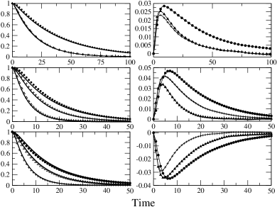
Figure 1: A comparison of the multiple-time correlation function $g^{(2)}$, the factored form $g^{(2)}_{f}$ and their difference as a function of wave vector pair $(m,n)$ and time cross-section $(t_{1},t_{2})$. The left hand side panels contain the simulation results for $g^{(2)}$ (unconnected symbols) and $g^{(2)}_{f}$ (lines), and the right hand side panels contain plots of $g^{(2)}-g^{(2)}_{f}$. In all panels, the unconnected dots, crosses and triangles correspond to the simulation results for time cross sections $(t,t)$, $(3t,t)$ and $(t,3t)$, respectively. The results in the top, middle and bottom rows are for wave vector sets $(1,2)$, $(1,3)$ and $(2,1)$, respectively. For clarity in the figures, the $96\%$ confidence intervals, estimated to be roughly $0.002$, have been omitted.

This difference should be well-reproduced by the mode-coupling correction term in Eq. 57, although this has not yet been verified.

IV.2.2 Multiple-point correlation function

Although it is certainly possible to calculate the leading order mode-coupling correction term in Eq. 57 analytically using hydrodynamic forms for the collective correlation functions $G_{11}^{cc}(t)$, the calculation is tedious due to the sum over different collective modes $B_{i}$. However in order to validate the applicability of the mode-coupling theory in the calculation of the first order correction terms $F^{mc}_{3}$, we examine the quality of the predicted form of the multiple-point correlation function

$$G_{21}^{ss}( \hat{N}_{1}(\mathbf{k}-\mathbf{q})\hat{N}(\mathbf{q});\hat{N}_{1}(\mathbf{k});t)$$ (68)

$$\equiv\left\langle\hat{N}_{1}(\mathbf{k}-\mathbf{q},t)\hat{N}(\mathbf{q},t)\hat{N}^{*}_{1}(\mathbf{k})\right\rangle-\frac{S(\mathbf{q})}{\langle N\rangle}F_{s}(\mathbf{k},t),$$

where $S(\mathbf{q})=\langle\hat{N}(\mathbf{q})\hat{N}^{*}(\mathbf{q})\rangle$ is the static structure factor, against direct numerical calculation (note: in Eq. 68 we took the thermodynamic limit). From Eq. 59, we see that this correlation function is approximately given by

$$G_{21}^{N_{1}N;N_{1}}(\mathbf{k}-\mathbf{q},\mathbf{q};t)=\int_{0}^{t}d\tau\;F_{s}(\mathbf{k}-\mathbf{q},t-\tau)$$ (69)

$$\qquad\times G_{11}^{NB_{j}}(\mathbf{q},t-\tau)M_{21}^{N_{1}B_{j};N_{1}}(\mathbf{k}-\mathbf{q},\mathbf{q};\mathbf{k})F_{s}(\mathbf{k},\tau),$$

where $B_{j}$ runs over the set $\{N,P_{l},H\}$ or some variant of it. Note that with this choice of collective densities, the computation of Eq. 69 requires the calculation of $3$ coupling vertices $M_{21}^{N_{1}N;N_{1}}$, $M_{21}^{N_{1}P_{l};N_{1}}$, and $M_{21}^{N_{1}H;N_{1}}$, as well as the input of the collective linear-linear time correlation functions $G_{11}^{NN}$, $G_{11}^{NP_{l}}$, and $G_{11}^{NH}$. In principle, analytical forms of the $G_{11}$ time correlation functions can be utilized in the hydrodynamic regime with transport coefficients either fitted from simulation data or taken from kinetic theory. Given the simplicity and ease of numerically calculating the $G_{11}$ with excellent precision, we have chosen to evaluate the convolution integrals in Eq. 69 by numerically integrating simulation data using a version of Simpson’s rule that allows interpolation of data. From time-inversion symmetry, $M_{21}^{E}=0$ for $B_{j}=N$ or $H$, and it is evident that the only coupling at “Euler” order arises for $B_{j}=P_{l}$. However, as noted for the case of multiple-point correlation functions of purely collective densities in Ref. VanZonSchofield02b, , the inclusion of the additional couplings to $N$ and $H$ arising at “dissipative” order $M_{21}^{D}$ is essential if quantitatively accurate predictions are desired. It may appear at first glance that the dissipative contributions are negligible in the limit of small wave vectors since they introduce additional factors of $k_{0}$. In fact the overall order of the multiple-point correlation functions is determined by a wave vector-dependent prefactor multiplied by the convolution of the two-point, single time interval correlation functions $G_{11}$. The time convolution of these correlation functions can give rise to additional factors of wave vector depending on their symmetry properties, so that the overall contribution of the $P_{l}$ and $N$ or $H$ coupling are comparable in magnitude.

The evaluation of the dissipative contribution to coupling vertices $M_{21}^{N_{1}N;N_{1}}$ and $M_{21}^{N_{1}H;N_{1}}$ requires external input. In the appendix, these vertices are evaluated in the small wave vector limit by relating the dissipative vertices to the Enskog self-diffusion coefficient and its derivatives with respect to thermodynamic parameters. The predictions are therefore free of any adjustable parameters and constitute a rigorous test of the mode-coupling theory. The results of the comparison are shown in Fig. 2.

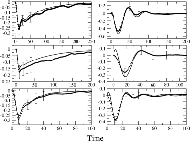
Figure 2: A comparison of simulated (unconnected dots) and predicted (solid lines) values of $G_{21}(t)$ as a function of $t$. The results in the top row correspond to wave vectors pairs $(1,2)$ and $(2,1)$ from left to right, the middle row correspond to $(1,3)$ and $(3,1)$, and the bottom row to $(2,3)$ and $(3,2)$.

Note that although the data are a bit noisy, the theoretical predictions generally fall within the confidence intervals of the simulated data except at very short times ($t\sim 2t_{e}$) where one expects the theory to break down due to the instantaneous approximation of the coupling vertices.

V Summary

In this paper, a mode-coupling theory was presented in which multiple point and multiple-time correlation functions for collective densities and tagged particle densities are expressed in terms of ordinary two-point, single-time interval correlation functions and a set of vertices. The theory developed here does not assume that fluctuating forces (noise) are Gaussian distributed and, in principle, does not require an ansatz to obtain self-consistent equations. Furthermore, unlike kinetic theories, it is not restricted to low densities and should be applicable to dense fluids where cooperative motions of particles and collective modes are important.

The formalism is based on projection operator techniques, which, for ordinary two-point, single-time correlation functions, lead to a generalized Langevin equation in which the memory function decays on a microscopic time scale (Eq. 6). The simple extension of the projection operator formalism to multiple-time correlation functions of tagged particle densities is complicated by the fact that the fluctuating forces appearing in the generalized Langevin equation do not obey Gaussian statistics. Furthermore, multiple-time correlations of the fluctuating force can in fact have a slow decay when the time arguments of these forces become comparable. In order to treat multiple-time correlation functions of fluctuating forces properly, the correlation functions were manipulated so that the time arguments of all fluctuating forces appearing in the correlations were guaranteed to be well-separated, ensuring that all memory functions which arise in the mode-coupling theory decay to zero on a molecular time scale. This construction allows equations which are local in time to be obtained which relate the multiple-time correlation function to two-time but multiple-point correlations coupled by essentially time-independent vertices. These expressions, in turn, can be written as convolutions of two-point, single time interval “propagators” coupled by time-independent vertices. These propagators can either be taken directly from experiment, simulation, or can be solved self-consistently within the mode-coupling formalism. The vertices, which are composed of a static part (Euler term) and a generalized transport coefficient, can similarly be calculated from kinetic theory or taken from molecular dynamics and Monte-Carlo simulations.

The equations for higher-order correlation functions contain an infinite sum of terms which can be made tractable for systems with a finite correlation length by applying a cumulant expansion technique pioneered by Oppenheim and co-workersMachtaOppenheim82 ; Schofieldetal92 ; SchofieldOppenheim92 termed the $N$-ordering method. The method was applied to obtain the leading order and first mode-coupling corrections of expressions for tagged-particle density multiple-time and mixed tagged/collective particle density multiple-point correlation functions designed to probe detailed aspects of the relaxation profile of glassy systems.

The mode-coupling theory outlined here is the first step towards a fully microscopic theory applicable to molecular length scales that enables one to analyze the mapping of the dynamics in deterministic glassy systems to stochastic spin model of glasses, as well as to define sub-ensembles via filters based on dynamical and spatial properties to probe dynamic heterogeneities, clustering properties and many other aspects of the dynamics of frustrated systems.

Appendix A Evaluation of the mode-coupling vertices

As mentioned in the main text, the vertices required for the calculation of the mode-coupling correction to the factorization of the multiple-time correlation function $F_{3}(t_{1},t_{2})$ are $M_{21}^{N_{1}P_{l};N_{1}}$, $M_{21}^{N_{1}N;N_{1}}$ and $M_{21}^{N_{1}H;N_{1}}$, where the general form of the vertex $M_{21}^{ss}$ is

$$M_{21}^{ss} =M_{21}^{Ess}+M_{21}^{Dss}$$

$$M_{21}^{Ess} =\left\langle{\cal L}Q_{2}^{s}Q_{1}^{s*}\right\rangle\cdot K_{11}^{ss-1}$$ (70)

$$M_{21}^{Dss} =-\int_{0}^{\infty}d\tau\left\langle\varphi_{2}^{s}(\tau)\varphi_{1}^{s*}\right\rangle\cdot K_{11}^{ss-1},$$ (71)

where $M_{21}^{E}$ is referred to as the “Euler” contribution to the vertex, $M_{21}^{D}$ is the “dissipative” part of the vertex, and $\varphi(t)$ is the fluctuating force defined in Eq. 10.

Examining first the Euler contributions $M_{21}^{Ess}$, we note that since $\left\langle{\cal L}Q_{2}^{s}Q_{1}^{s*}\right\rangle=-\left\langle Q_{2}^{s}{\cal L}Q_{1}^{s*}\right\rangle$, we have

$$M_{21}^{Ess}( \hat{N}_{1}(\mathbf{k}-\mathbf{q})B(\mathbf{q});\hat{N}_{1}(\mathbf{k}))=$$

$$\frac{i}{m}\left\langle Q_{2}^{s}(\hat{N}_{1}(\mathbf{k}-\mathbf{q}),B(\mathbf{q}))\mathbf{P}_{1}^{*}(\mathbf{k})\right\rangle\cdot\mathbf{k}.$$ (72)

¿From the time-reversal symmetry properties of the correlation functions, we see that $M_{21}^{Ess}=0$ for $B=N$ and $B=H$, and for $B=P_{l}$ we find

$$M_{21}^{Ess}( \hat{N}_{1}(\mathbf{k}-\mathbf{q})P_{l}(\mathbf{q});\hat{N}_{1}(\mathbf{k}))=\frac{i\mathbf{k}\cdot\hat{\mathbf{q}}}{\beta}.$$ (73)

Evaluation of the dissipative vertices $M_{21}^{Dss}$ requires the calculation of the linear $\varphi_{1}$ and bi-linear $\varphi_{2}$ fluctuating forces. For the linear fluctuating force, we have (in the thermodynamic limit)

$$\varphi_{1}(\mathbf{k},t) =e^{\mathcal{P}^{\perp}{\cal L}t}\mathcal{P}^{\perp}{\cal L}\hat{N}_{1}(\mathbf{k})$$

$$=e^{\mathcal{P}^{\perp}{\cal L}t}i\mathbf{P}_{1}(\mathbf{k})\cdot\hat{\mathbf{k}}/m,$$ (74)

and the bi-linear fluctuating force is

$$\varphi_{2}(\mathbf{k}-\mathbf{q},\mathbf{q};t) =e^{\mathcal{P}^{\perp}{\cal L}t}\mathcal{P}^{\perp}{\cal L}Q_{2}^{s}(\mathbf{k}-\mathbf{q},\mathbf{q}),$$

where $\mathcal{P}^{\perp}$ is a projection operator that projects onto a subspace orthogonal to that spanned by the multi-linear basis set $Q_{\alpha}$. Noting that (in the thermodynamic limit)

$$Q_{2}^{s}(\hat{N}_{1}(\mathbf{k}-\mathbf{q})\hat{N}(\mathbf{q})) =\hat{N}_{1}(\mathbf{k}-\mathbf{q})\hat{N}(\mathbf{q})-\frac{S(\mathbf{q})}{\langle N\rangle}\hat{N}_{1}(\mathbf{k})$$

$$Q_{2}^{s}(\hat{N}_{1}(\mathbf{k}-\mathbf{q})P_{l}(\mathbf{q})) =\hat{N}_{1}(\mathbf{k}-\mathbf{q})P_{l}(\mathbf{q})$$

$$Q_{2}^{s}(\hat{N}_{1}(\mathbf{k}-\mathbf{q})H(\mathbf{q})) =\hat{N}_{1}(\mathbf{k}-\mathbf{q})H(\mathbf{q})$$ (75)

and $\mathcal{P}^{\perp}\hat{N}_{1}(\mathbf{k}-\mathbf{q})\mathbf{P}(\mathbf{q})=0$, we see that at $t=0$, the bilinear fluctuating forces are

$$\varphi_{2}^{s}(\hat{N}_{1}(\mathbf{k}-\mathbf{q})\hat{N}(\mathbf{q})) =\frac{i(\mathbf{k}-\mathbf{q})}{m}\cdot\mathbf{P}_{1}(\mathbf{k}-\mathbf{q})\hat{N}(\mathbf{q})$$

$$\qquad\qquad-\frac{S(\mathbf{q})}{\langle N\rangle}\frac{i\mathbf{k}}{m}\cdot\mathbf{P}_{1}(\mathbf{k})$$

$$\varphi_{2}^{s}(\hat{N}_{1}(\mathbf{k}-\mathbf{q})P_{l}(\mathbf{q})) =\frac{i(\mathbf{k}-\mathbf{q})}{m}\cdot\mathcal{P}^{\perp}\mathbf{P}_{1}(\mathbf{k}-\mathbf{q})\mathbf{P}(\mathbf{q})\cdot\hat{\mathbf{q}}$$

$$\qquad+\mathcal{P}^{\perp}\hat{N}_{1}(\mathbf{k}-\mathbf{q}){\cal L}\mathbf{P}(\mathbf{q})\cdot\hat{\mathbf{q}}$$

$$\varphi_{2}^{s}(\hat{N}_{1}(\mathbf{k}-\mathbf{q})H(\mathbf{q})) =\frac{i(\mathbf{k}-\mathbf{q})}{m}\cdot\mathcal{P}^{\perp}\mathbf{P}_{1}(\mathbf{k}-\mathbf{q})H(\mathbf{q})$$

$$\qquad+\mathcal{P}^{\perp}\hat{N}_{1}(\mathbf{k}-\mathbf{q}){\cal L}H(\mathbf{q}).$$

Inserting these results into the expressions for the dissipative vertices and expanding the resulting expressions in powers of the base wave vector $k_{0}$, one finds

$$M_{21}^{ssN_{1}N;N_{1}} =-\frac{(\mathbf{k}-\mathbf{q})\cdot\mathbf{k}}{m^{2}}\int_{0}^{\infty}d\tau\left\langle\mathbf{P}^{x}_{1}(\tau)\mathbf{P}^{x}_{1}\hat{N}\right\rangle$$

$$\qquad+\frac{k^{2}S(\mathbf{q})}{m^{2}\langle N\rangle}\int_{0}^{\infty}d\tau\left\langle\mathbf{P}^{x}_{1}(\tau)\mathbf{P}^{x}_{1}\right\rangle+O(k_{0}^{3})$$

$$M_{21}^{ssN_{1}P_{l};N_{1}} =O(k_{0}^{3})$$

$$M_{21}^{ssN_{1}H;N_{1}} =-\frac{(\mathbf{k}-\mathbf{q})\cdot\mathbf{k}}{m^{2}}\int_{0}^{\infty}d\tau\left\langle\mathbf{P}^{x}_{1}(\tau)\mathbf{P}^{x}_{1}H\right\rangle$$

$$\qquad-\frac{\mathbf{k}\cdot\mathbf{q}}{m}\int_{0}^{\infty}d\tau\left\langle\mathbf{j}_{H}(\tau)\mathbf{P}_{1}\right\rangle+O(k_{0}^{3}),$$

where we have defined $i\mathbf{q}\cdot\mathbf{j}_{H}(\mathbf{q})=-2\beta/\sqrt{6}\,\mathcal{P}^{\perp}{\cal L}\hat{E}(\mathbf{q})$. Noting that the Green-Kubo expression for the self-diffusion coefficient $m^{2}D=\int_{0}^{\infty}dt\,\langle\mathbf{P}^{x}_{1}(t)\mathbf{P}_{1}^{x}\rangle$ and that $\langle A\hat{N}\rangle=\partial\langle A\rangle/\partial(\beta\mu)$ and $\langle A\hat{E}\rangle=-\partial\langle A\rangle/\partial\beta$, where $\mu$ is the chemical potential of the system, allows us to write

$$M_{21}^{ssN_{1}N;N_{1}} =-(\mathbf{k}-\mathbf{q})\cdot\mathbf{k}\left(\frac{\partial D}{\partial\beta\mu}\right)_{\beta}+\frac{S(0)}{\langle N\rangle}Dk^{2}+O(k_{0}^{3})$$

$$M_{21}^{ssN_{1}H;N_{1}} =-\frac{(\mathbf{k}-\mathbf{q})\cdot\mathbf{k}}{\sqrt{6}}\left[3\left(\frac{\partial D}{\partial\beta\mu}\right)_{\beta}+2\beta\left(\frac{\partial D}{\partial\beta}\right)_{\beta\mu}\right]$$

$$\qquad-\frac{\mathbf{k}\cdot\mathbf{q}}{m}\int_{0}^{\infty}d\tau\left\langle\mathbf{j}_{H}(\tau)\mathbf{P}_{1}\right\rangle+O(k_{0}^{3}).$$

The dissipative vertex $M_{21}^{ssN_{1}H;N_{1}}$ contains a new transport coefficient $\int_{0}^{\infty}d\tau\left\langle\mathbf{j}_{H}(\tau)\mathbf{P}_{1}\right\rangle$ which could, in principle, be evaluated by doing a short-time expansion or using uncorrelated collisions in a kinetic theory. Nonetheless, we expect this contribution to be very small since $\langle\mathbf{j}_{H}(\tau)\mathbf{P}\rangle$ is strictly zero due to the projection operator $\mathcal{P}^{\perp}$. In the numerical work in the main text, we have set this term to zero.

Using the Enskog form for the self-diffusion coefficient and the Carnahan-Starling equation of state, we find that

$$\left(\frac{\partial D}{\partial\beta\mu}\right)_{\beta} =-\frac{D}{g(a)}\frac{\bar{\eta}(2\bar{\eta}-5)}{2(1-\bar{\eta})^{4}}\frac{S(0)}{\langle N\rangle}$$

$$\left(\frac{\partial D}{\partial\beta}\right)_{\beta\mu} =-\frac{D}{2\beta}+\frac{D}{g(a)}\frac{\bar{\eta}(2\bar{\eta}-5)}{2(1-\bar{\eta})^{4}}\frac{3S(0)}{2\beta\langle N\rangle}.$$ (76)

Thus, the $M_{21}$ vertices used in the main text are:

$$M_{21}^{ssN_{1}N;N_{1}} =\frac{DS(0)}{\langle N\rangle}\left[\frac{\mathbf{k}\cdot(\mathbf{k}-\mathbf{q})}{g(a)}\frac{\bar{\eta}(2\bar{\eta}-5)}{2(1-\bar{\eta})^{4}}+k^{2}\right]$$

$$M_{21}^{ss}(\hat{N}_{1}P_{l};N_{1}) =\frac{i\mathbf{k}\cdot\hat{\mathbf{q}}}{\beta}$$

$$M_{21}^{ssN_{1}H;N_{1}} =\frac{D(\mathbf{k}-\mathbf{q})\cdot\mathbf{k}}{\sqrt{6}}.$$

References

• (1) W. Kob, C. Donati, S. Plimpton, P. Poole and S. Glotzer, Phys. Rev. Lett. 79, 2827 (1997).
• (2) R. Yamamoto and A. Onuki, Phys. Rev. E 58, 3315 (1998).
• (3) R. Yamamoto and A. Onuki, Phys. Rev. Lett. 81, 4915 (1998).
• (4) B. Doliwa and A. Heuer, Phys. Rev. Lett. 80, 4915 (1998).
• (5) W. Kob, J. Phys.: Condens. Matter 11, R85 (1999).
• (6) R. Yamamoto and A. Onuki, Intl. J. Modern Phys. C 10, 1553 (1999).
• (7) S. Sjödin and A. Sjölander, Phys. Rev. A 18, 1723 (1978).
• (8) R. Böhmer, G. Hinze, G. Diezemann, B. Geil and H. Sillescu, Europhys. Lett. 36, 55 (1996).
• (9) U. Tracht et al., Phys. Rev. Lett. 81, 2727 (1998).
• (10) A. H. Marcus, J. Schofield and S. A. Rice, Phys. Rev. E 60, 5725 (1999).
• (11) E. R. Weeks, J. C. Crocker, A. C. Levitt, A. Schofield and D. A. Weitz, Science 287, 627 (2000).
• (12) A. Heuer, Phys. Rev. E 56, 730 (1997).
• (13) A. Heuer and K. Okun, J. Chem. Phys. 106, 6176 (1997).
• (14) B. Doliwa and A. Heuer, J. Phys. C: Condens. Matter 11, A277 (1999).
• (15) R. van Zon and J. Schofield, Phys. Rev. E 65, 011106 (2002).
• (16) B. J. Alder and T. E. Wainwright, J. Phys. Soc. Japan (Suppl.) 26, 267 (1968).
• (17) B. J. Alder and T. E. Wainwright, Phys. Rev. Lett. 18, 988 (1969).
• (18) I. Michaels and I. Oppenheim, Physica A 81, 454 (1975).
• (19) J. Schofield and I. Oppenheim, Physica A 187, 210 (1992).
• (20) P. Schramm and I. Oppenheim, Physica A 137, 81 (1986).
• (21) J. Machta and I. Oppenheim, Physica A 112, 361 (1982).
• (22) J. Schofield, R. Lim and I. Oppenheim, Physica A 181, 89 (1992).
• (23) N. G. van Kampen, Stochastic Processes in Physics and Chemistry, Revised and enlarged ed. (North Holland, Amsterdam, 1992).
• (24) T. Keyes and I. Oppenheim, Phys. Rev. A 8, 937 (1973).
• (25) T. Keyes, Principles of mode-mode coupling theory, in Statistical Mechanics, Part B, edited by B. J. Berne, New York, 1977, Plenum Press.
• (26) J. Qian, R. Hentschke and A. Heuer, J. Chem. Phys. 110, 4514 (1999).
• (27) G. H. Frederickson and H. C. Andersen, Phys. Rev. Lett. 53, 1244 (1984).
• (28) G. Fredrickson and H. Andersen, J. Chem. Phys. 83, 5822 (1985).
• (29) S. J. Pitts, T. Young and H. C. Andersen, J. Chem. Phys. 113, 8671 (2000).
• (30) S. J. Pitts and H. C. Andersen, J. Chem. Phys. 114, 1101 (2001).
• (31) F. Ritort and P. Sollich, Adv. Phys. 52, 219 (2003).
• (32) R. van Zon and J. Schofield, J. Chem. Phys. 122, yyyyyy (2005).
• (33) I. M. de Schepper and E. G. D. Cohen, Phys. Rev. A 22, 287 (1980).
• (34) B. Kamgar-Parsi, E. G. D. Cohen and I. M. de Schepper, Phys. Rev. A 35, 4781 (1987).
• (35) R. van Zon and J. Schofield, Phys. Rev. E 65, 011107 (2002).
• (36) S. Chapman and T. Cowling, Mathematical Theory of Non-uniform Gases, 3rd edition (University Press, Cambridge, 1970)
• (37) N. Carnahan and K. Starling, J. Chem. Phys. 51, 635 (1969).