Higher Landau levels contribution
to the energy of interacting electrons in a quantum dot

Abstract

Properly regularized second-order degenerate perturbation theory is applied to compute the contribution of higher Landau levels to the low-energy spectrum of interacting electrons in a disk-shaped quantum dot. At “filling factor” near 1/2, this contribution proves to be larger than energy differences between states with different spin polarizations. After checking convergence of the method in small systems, we show results for a 12-electron quantum dot, a system which is hardly tractable by means of exact diagonalization techniques.

I Introduction

The relevant energy scales entering the Hamiltonian of an $N$-electron system in a quantum dot (qdot) and a magnetic field are the following: the cyclotronic energy $\hbar\omega_{c}\sim B$, the dot confinement energy $\hbar\omega_{0}$, and the Coulomb characteristic energy $e^{2}/(\kappa l_{B})\sim\sqrt{B}$. In strong enough fields, the spacing between Landau levels (LLs), given by $\hbar\omega_{c}$, is much greater than any other scale, and one can restrict the Hilbert space to functions built on one-particle states from the first LL. This is the 1LL approximation Chakraborty , which has been widely used to obtain exact solutions Laughlin1 , to construct the famous $\nu=1/3$ FQHE functions Laughlin2 , later extended to other filling factors by means of the Composite Fermion recipe Jain2 and, in general, has been used to numerically diagonalize the interacting Hamiltonian Chakraborty .

The inclusion of higher LLs in numerical calculations turns out to be prohibitive, even for relatively “small” systems. Consider, for example, N=12 electrons in a qdot at “filling factor” near 1/2, i.e. when the angular momentum of the electron droplet is $L=-132$. Out of only 78 one-particle states (orbitals) in the 1LL, one can construct 674585 Slater determinants, which conform the truncated basis for the 12-particle system in the 1LL approximation. Taking 78 additional orbitals from each of the next two LLs causes the basis dimension to be raised to more than 172 millions, and the diagonalization of the Hamiltonian matrix becomes a very hard computational task.

In the present paper, we show that a way to circumvent the diagonalization of these large matrices is the use of properly renormalized degenerate perturbation theory (PT). We stress that, unlike Monte Carlo and other methods focusing on the properties of a particular state, by means of PT we obtain, in a single calculation, an approximation to the energy spectrum and the corresponding wave functions of the system.

The interest in computing the higher LL contribution to the energies relies in the fact that, for intermediate filling factors, this contribution may be even larger than energy differences between states with different spin polarizations prb . Thus, a correct description of spin excitations in a system of interacting electrons should take account of higher LL effects. Recent work on the issue of spin excitations in qdots Haw has stressed the importance of the second LL at $\nu\approx 2$, but at lower $\nu$ the higher LL effects are commonly ignored.

The plan of the paper is as follows. In the next two sections a brief summary of PT and its regularization by means of Shank extrapolants Shank and the Principle of Minimal Sensitivity PMS is included for completeness. For simplicity, only spin-polarized systems will be studied, but any other spin-polarization sector may be treated as well. Section IV is devoted to the results. The 2- and 6-electron dots are used as benchmarks where regularized second-order PT (PT2) is compared with exact or variational results. After validation, the method is applied to the 12-electron system mentioned above. Concluding remarks are given at the end of the paper.

II Degenerate perturbation theory

The 1LL approximation can be seen, from another point of view, as first-order degenerate perturbation theory. In fact, writing the Hamiltonian in the form: $H=H_{0}+V$, where $H_{0}$ describes free (spin-polarized) electrons in a magnetic field, and $V=V_{conf}+V_{coul}$ accounts for the external confinement and Coulomb interactions, the Hamiltonian matrix in the 1LL approximation,

$$H_{ij}^{(1)}=\langle S_{i}|H|S_{j}\rangle=E_{0}\delta_{ij}+\langle S_{i}|V|S_{j}\rangle,$$ (1)

where $E_{0}=N\hbar\omega_{c}/2$ and $S_{i},~{}S_{j}$ are Slater determinants made up from 1LL orbitals, may be seen as the secular matrix of first-order degenerate perturbation theory QM . The degeneracy subspace is spanned by the $S_{i}$.

Corrections to (1) are computed in the standard form QM . The second-order matrix is given by:

$$H_{ij}^{(2)}=E_{0}\delta_{ij}+\langle S_{i}|V+\sum_{Z}\frac{V|Z\rangle\langle Z|V}{E_{0}-E_{0}(Z)}|S_{j}\rangle,$$ (2)

where the sum runs over eigenfunctions of $H_{0}$ in the orthogonal subspace, $\langle Z|S_{i}\rangle=0$, and $E_{0}(Z)=\langle Z|H_{0}|Z\rangle$.

We will use Eq. (2) to compute higher LLs contributions to the energy spectrum of an N-electron qdot. Notice that the dimension of the secular equation is not increased by the inclusion of the second-order corrections. For the largest systems, an energy cutoff, $E_{0}(Z)-E_{0}\leq K_{cut}~{}\hbar\omega_{c}$, will be imposed to limit the number of states entering the sum. We will show results with $K_{cut}=2$, i. e. three LLs will be included.

II.1 The orthogonal subspace

One can explicitly use the fact that $V_{conf}$ and $V_{coul}$ are, respectively, one- and two-body operators, and exploit their symmetries (conservation of total angular momentum) in order to carry out the sum only over intermediate states, $Z$, having nonvanishing matrix elements with one of the external Slater functions, for example $\langle Z|V|S_{j}\rangle\neq 0$.

Figure 1: Slater functions in the degeneracy subspace, $S_{j}$, and in the orthogonal subspace, $Z$, entering the sum in Eq. (2). The example is for a 4-electron system.

In Fig. 1, we have illustrated this statement for the simple 4-electron system. The top of the figure shows the occupation corresponding to a given $S_{j}$. Then, the sum will contain functions $Z_{1}$, where one occupied orbital of $S_{j}$ is raised to an orbital in a higher LL (with the same angular momentum, $l$). The sum will also contain functions $Z_{2}$, where two occupied levels of $S_{j}$ are moved to higher LLs. And, finally, functions $Z_{3}$ in which one occupied level of $S_{j}$ is moved to an empty level in the 1LL and a second occupied orbital is moved to a higher LL shall also be included. In the first case, both the matrix elements of $V_{conf}$ and $V_{coul}$ could be nonzero, whereas in the later two cases only $V_{coul}$ could have nonvanishing matrix elements.

III Regularization of the perturbative series

To renormalize the perturbative series (usually an asymptotic series) many recipes have been invented. In the present paper, we will try Shank extrapolants Shank and the principle of minimal sensitivity (PMS) PMS . A variant of the later procedure has been recently applied to compute the correlation energy of the Coulomb gas Sang .

III.1 Shank extrapolants

Shank extrapolants Shank are designed to accelerate the convergence of numerical series. For any three contiguous values, $E_{i}$, $E_{i+1}$ and $E_{i+2}$, we define the extrapolant:

$$F_{i}=\frac{E_{i}E_{i+2}-E_{i+1}^{2}}{E_{i}+E_{i+2}-2E_{i+1}}.$$ (3)

From the series of extrapolants (which will be called first order) one can construct the second-order extrapolants, etc. In our case, we have only three values of energy, $E_{0}$, $E_{1}$ and $E_{2}$, obtained from PT0, PT1 and PT2, and thus there will be only one extrapolant, $F_{0}$.

III.2 The principle of minimal sensitivity

The PMS starts from the obvious fact that if the Hamiltonian is made to depend on an artificial trivial parameter $\alpha$: $H\to H(\alpha)$, then the exact eigenvalues will satisfy the equations:

$$\frac{{\rm d}E}{{\rm d}\alpha}=0.$$ (4)

The perturbative expansion may not, however, respect these constraints. The PMS states that an optimal choice for $\alpha$ at a given perturbative order is the value at which Eq. (4) is satisfied.

In our $N$-electron system, described by the Hamiltonian:

$$H = \sum_{i}\left(\frac{p_{i}^{2}}{2m}+\frac{m\omega_{c}^{2}}{8}r_{i}^{2}+\frac{\hbar\omega_{c}}{2}l_{i}\right)+\frac{m\omega_{0}^{2}}{2}\sum_{i}r_{i}^{2}$$ (5)

$$+ \frac{e^{2}}{\kappa}\sum_{i<j}\frac{1}{r_{ij}},$$

the introduction of trivial terms and a scaling of coordinates lead to:

$$H = \frac{\hbar\omega_{c}^{\prime}}{2}\sum_{i}\left(\frac{p_{i}^{2}}{2}+\frac{r_{i}^{2}}{2}+l_{i}\right)$$ (6)

$$+ \frac{\hbar}{\omega_{c}^{\prime}}\left(\omega_{0}^{2}+\frac{\omega_{c}^{2}}{4}-\frac{\omega_{c}^{\prime 2}}{4}\right)\sum_{i}r_{i}^{2}$$

$$+ \left(\frac{\hbar\omega_{c}}{2}-\frac{\hbar\omega_{c}^{\prime}}{2}\right)L+\frac{e^{2}}{\kappa}\sqrt{\frac{m\omega_{c}^{\prime}}{2\hbar}}\sum_{i<j}\frac{1}{r_{ij}},$$

where $\hbar\omega_{c}^{\prime}$ is an artificial parameter (magnetic field) and $L=\sum_{i}l_{i}$. The first sum in Eq. (6) will be taken as the unperturbed Hamiltonian, $H_{0}$, and the subsequent terms as the perturbation, $V$. Notice that the term $(\hbar\omega_{c}/2-\hbar\omega_{c}^{\prime}/2)L$ in $V$ will give no contribution to the second-order correction because $[H_{0},L]=0$.

The parameter $\hbar\omega_{c}^{\prime}$ will be fixed from the condition (4). Working whithin PT1, one can interpret $\hbar\omega_{c}^{\prime}$ as a variational parameter. In PT2, however, the point in which (4) is satisfied in our examples is a local maximum, as will be seen below.

IV Results

The qdot parameters to be used are borrowed from Ref. prb, . GaAs effective mass, $m=0.067m_{0}$, and relative dielectric constant $\kappa=12.5$ are employed. The confinement potential is parabolic with $\hbar\omega_{0}=3$ meV. The bare Coulomb interaction is weakened by a factor 0.8 to approximately account for quasi-bidimensionality (instead of exact bidimensionality). We will only deal with spin-polarized systems, thus the Zeeman energy is a trivial constant and will not be included.

IV.1 Two electrons

In the two-electron dot, calculations may be carried out semi-analytically. The results for the ground-state energy of the triplet state with $L=-1$ at $B=8$ T are the following: $E_{0}=13.82$, $E_{1}=20.28$, and $E_{2}=20.16$ meV. The exact energy is $E=20.17$ meV. Notice that the higher LL contribution to $E$ is -0.12 meV, and that $E_{2}$ is very close to the exact value.

Regularization of the perturbative series by means of the Shank extrapolant yields a value $F_{0}$ which practically coincides with $E_{2}$. The difference lies in the fifth significant figure, not written above.

On the other hand, as a function of the PMS parameter, $B^{\prime}$, we obtain the curves shown in Fig. 2 for the magnitudes $E_{1}(B^{\prime})$ and $E_{2}(B^{\prime})$.

Figure 2: $E_{1}$ and $E_{2}$ as a function of $B^{\prime}$ for the two-electron system at $B=8$ T.

Note that the position of the minimum in $E_{1}(B^{\prime})$ practically coincides with the position of the maximum in $E_{2}(B^{\prime})$. These are the physically acceptable values of $B^{\prime}$ according to (4). Note also that the PMS-regularized ground state energy has the same significant figures as the unregularized second-order result, $E_{2}(B)$.

IV.2 Six electrons

The exact diagonalization (variational) results of Ref. prb, show that at $B=8$ T (filling factor near 1/2) the contribution of the second and third LLs to the energy eigenvalues is around -0.4 meV, i. e. around -0.06 meV per electron, as in the two electron system. This magnitude is greater than the energy differences between states with different spin polarizations.

The lowest spin-polarized states in each angular momentum tower (the yrast spectrum) are shown in Fig. 3. Energy jumps between adjacent angular momentum states are about 0.6 meV. The PT2 results are shown to lay 0.04 meV below the variational ones, that is, almost inside the estimated error bars which are about 0.03 meV. These PT2 results are obtained with $K_{cut}=2$, as mentioned above.

Figure 3: Variational and PT2 results for the low-lying states in the 6-electron dot. $B=8$ T.

Regularization of the perturbative series leads to results very similar to those in the two-electron dot: the significant figures (in this case five) are not changed. This means that one can in practice estimate the ground state energy from the PT2 result.

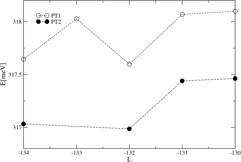
Figure 4: PT1 and PT2 estimates of the low-lying spin-polarized energy levels of twelve electrons. $B=10$ T.

IV.3 Twelve electrons

We show in Fig. 4 the perturbative low-lying spectrum for the 12-electron dot. In this situation, the perturbative results are the only ones at our disposal because exact diagonalization is practically impossible. The magnetic field is 10 T in this figure. Notice the energy jumps between adjacent angular momentum states, as in the 6-electron dot. The contribution of the higher LLs to the energy eigenvalues is around -0.6 meV, that is, -0.05 meV per electron.

Only the lowest eigenvalues in each angular momentum tower are drawn in Fig. 4, but the next 20-30 eigenvalues are reliable as well. The generation of the second-order matrix, Eq. (2), for a single $L$ value takes around one week CPU time in a small computer cluster with ten processors at 2.4 GHz. The PT2 matrix is a factor of ten less sparse than the PT1 matrix, occupying around 15 GB of hard disk. Consequently, diagonalization by means of a Lanczos algorithm takes a factor of ten more time.

V Concluding remarks

We have shown the feasibility of computing the energy eigenvalues and eigenfunctions of relatively large electronic quantum dots in a magnetic field by using second-order degenerate perturbation theory to take account of the contribution of the higher LLs. This contribution proves to be of the same order of energy differences between states with different spin polarizations. The constructed effective Hamiltonian in the 1LL can be diagonalized by means of standard Lanczos techniques. We presented calculations for the spin-polarized states of a 12-electron quantum dot at filling factor near 1/2. When three LLs are included, the dimension of the truncated Hilbert space for this problem is larger than 170 millions.

From a more general point of view, a similar scheme could be applied to any problem with well differentiated energy scales, in which one could identify, at least approximately, degeneracy subspaces. Examples of such problems are the study of mixing between vibrational and electronic degrees of freedom in relatively large molecules, or the study of mixing between intra- and inter-shell excitations in relatively large nuclei.

- (1) T. Chakraborty and P. Pietilainen, The quantum Hall effects, Springer, New York, 1996.
- (2) R.B. Laughlin, Phys. Rev. B 27, 3383 (1983).
- (3) R.B. Laughlin, Phys. Rev. Lett. 50, 1395 (1983).
- (4) J.K. Jain and R.K. Kamilla in Composite fermions, ed. O. Heinonen, World Scientific, Singapore, 1988.
- (5) A. Gonzalez and R. Capote, Phys. Rev. B 66, 113311 (2002).
- (6) A. Wensauer, M. Korkusinski, and P. Hawrylak, Phys. Rev. B 67, 035325 (2003).
- (7) C.M. Bender and S.A. Orszag, Advanced Mathematical Methods for Scientists and Engineers. New-York, McGraw-Hill, 1978.
- (8) P.M. Stevenson, Phys. Rev. D 23, 2916 (1981).
- (9) L.D. Landau and E.M. Lifshits, Quantum Mechanics, non-relativistic theory. Oxford, Pergamon Press, 1977.
- (10) Sang Koo You and Noboru Fukushima, J. Phys. A: Math. Gen. 36, 9647 (2003).